Outer-Radius Catenoid Stability and Uniqueness of Minimal Graphs

April 17, 2026

Abstract

In this paper, we explore minimal surfaces and graphs in differential geometry. We derive the equation for a catenoid, a rotationally symmetric solution to the first variation of area functional for equidistant bounded discs. This analysis reveals two possible configurations for the catenoid, with an inner-radius and outer-radius catenoid that arise when the distance between the coaxial discs is below a critical threshold; we rigorously prove the stability of the outer-radius catenoid as the unique, area-minimizing surface. Additionally, we establish the rigidity and uniqueness of minimal (planar) graphs; we prove that the Dirichlet problem admits at most one minimal graph. Moreover, when the Dirichlet boundary curve lies in a plane, the corresponding minimal planar graph must reside entirely in the same plane.

Introduction

Plateau’s problem, first proposed in the late 18th century¹ , asks whether a surface of minimal area exists under specific boundary constraints. Solutions to this problem, minimal surfaces, have since been studied extensively and have applications in fields such as physics, molecular biology, and architecture; for instance, minimal surfaces are used to model the apparent horizon of black holes², describe the theoretical model of biomolecules³, and even inspire modern architecture⁴. As such, Differential Geometry, the broader context of minimal surfaces, remains a relevant field in mathematics, as it extends the familiar study of Euclidean geometry to higher-dimensional space to measure area, curvature, torsion, etc., using the tools of calculus, linear algebra, and topology.

This paper focuses on two specific cases of minimal surfaces: catenoids and minimal graphs. More specifically, we prove two main results: (i) that the outer-radius catenoid is stable and area-minimizing as the unique solution to Plateau’s problem, Theorem (4.2), and (ii) that the Minimal Graph Equation permits one unique solution, Theorem (5.3), implying that planar Dirichlet boundary conditions yield only the trivial planar minimal graph, in Corollary (5.1). While there exist previous proofs⁴ for the stability of the outer-radius catenoid, we provide a self-contained proof that avoids reliance on advanced background in Sturm-Liouville theory or Differential Geometry aside from that introduced in sections two and three, and is thus more attainable for a broader audience. Physically, regarding the stability of the catenoid, several soap ring experiments⁵^,⁶ demonstrate the existence of two potential catenoid configurations bounded by coaxial rings, but that only the outer-radius catenoid is stable and persists under a critical separation distance d^∗ between the rings; using the first and second variation of area functionals, we mathematically justify such observations.

In the Geometry of Surfaces section, we provide the necessary background in Differential Geometry to understand and prove the results of this paper. In section three, we investigate the context of Plateau’s problem and minimal surfaces, deriving important theorems in minimal surface theory for our main results. In section four, we present an overview of the catenoid and prove our first main result in Theorem (4.2) regarding the stability of the outer-radius catenoid. Finally, in section five, we introduce the Maximum Principle for linear elliptic equations and prove our second main result in Theorem (5.3) regarding the uniqueness of minimal graphs, concluding with Corollary (5.1).

Geometry of Surfaces

This section introduces the fundamental concepts in the geometry of surfaces to properly analyze minimal surfaces. Specifically, we need to answer the question of what defines the geometry of a surface? In its essence, a surface in $\mathbb{R}^3$ has three major properties: length, area, and curvature; the latter two will be critical for defining a minimal surface. However, to start, we need to establish a formal definition of a regular surface and its composition from a local parametrization.

Definition 2.1 (Local Parametrization).

Let $M$ represent a subset in $\mathbb{R}^2$ . A map $F_{u,v}:U\subseteq\mathbb{R}^2\rightarrow O\subseteq\mathbb{R}^3$ is called a local parametrization of $M$ if the following conditions are satisfied:

$F:U\rightarrow\mathbb{R}^3$ is $C^\infty$ ; that is, $F$ is infinitely differentiable with respect to the codomain $\mathbb{R}^3$ .
$F:U\rightarrow O$ is a homeomorphism; i.e., $F:U\rightarrow O$ is bijective, and both $F$ and $F^{-1}$ are continuous.
$\forall (u,v)\in U$ , the cross product
$\frac{\partial F}{\partial u} \times \frac{\partial F}{\partial v} \neq 0$

Note that the third condition in Definition 2.1 is necessary to establish the linear independence of the parametrization for $F:U\rightarrow\mathbb{R}^3$ ; i.e., the nonzero cross product implies that, at any point on $M\subseteq\mathbb{R}^3$ , the surface cannot locally collapse to a single point or curve and must permit local tangent planes everywhere. This property is vital for Definition 2.3.

Definition 2.2 (Regular Surface). A subset $M\in\mathbb{R}^3$ is called a regular surface if, $\forall p\in M$ , there exists an open subset $U\subseteq\mathbb{R}^2$ and a corresponding open subset $O\subseteq M$ containing $p$ such that $F:U\rightarrow O$ is a local parametrization.

Importantly, we need to establish a local coordinate system on the surface $M$ to examine its behavior in space; specifically, we need a basis to reference the curvature and geometry of $M$ around an arbitrary point $p$ . Conveniently, the partial derivatives of a local parametrization $F:U\rightarrow M$ are well-defined (nonzero) everywhere on $M$ and are thus of interest for defining a local (tangent) plane.

Definition 2.3 (Tangent Plane). Let $M\in\mathbb{R}^2$ be a regular surface and $p\in M$ a point. If $F(u,v):U\rightarrow M$ is a local parametrization around $p$ , then the tangent plane $T_pM$ at $p$ is defined as

$T_pM := \text{span} \left{ \frac{\partial F}{\partial u}(p), \frac{\partial F}{\partial v}(p) \right}$

Remark 2.1. $\forall p\in M$ , $\dim{T_pM}=2$ , since $\frac{\partial F}{\partial u} \nparallel \frac{\partial F}{\partial v}$ by Definition 2.1.

With the proper local coordinates, we can now proceed with analyzing the behavior and geometry of $M$ around a point $p$ ; namely, we can examine the properties of curvature, area and length associated with $M$ . The latter two are defined with respect to a local inner product; let $x=x_1e_1+x_2e_2+x_3e_3, y=y_1e_1+y_2e_2+y_3e_3\in\mathbb{R}^3$ . Then

$\left\langle x,y \right\rangle = \begin{bmatrix} x_1 & x_2 & x_3 \end{bmatrix} \begin{bmatrix} \left\langle e_1,e_1 \right\rangle & \left\langle e_1,e_2 \right\rangle & \left\langle e_1,e_3 \right\rangle \\ \left\langle e_2,e_1 \right\rangle & \left\langle e_2,e_2 \right\rangle & \left\langle e_2,e_3 \right\rangle \\ \left\langle e_3,e_1 \right\rangle & \left\langle e_3,e_2 \right\rangle & \left\langle e_3,e_3 \right\rangle \end{bmatrix} \begin{bmatrix} y_1 \\ y_2 \\ y_3 \end{bmatrix}$

such that $\left\langle x,y \right\rangle = x^T E y$ for basis matrix $E$ .

First Fundamental Form. As alluded to earlier, we can express area and length attributed to a regular surface $M$ using a local inner product; to do so, we must define the first fundamental form and its matrix definition.

Definition 2.4 (First Fundamental Form). If $M$ is a regular surface, the first fundamental form of $M$ is the inner product on $T_pM\times T_pM$ for all $p\in M$ , denoted as $g:T_pM\times T_pM\rightarrow\mathbb{R}$ .

Remark 2.2 (Matrix Form). Let $F(u_1,u_2)$ represent a local parametrization for a regular surface $M$ and $p\in M$ have tangent plane $T_pM$ . Then, for $x,y\in T_pM$ , by Definition 2.4, the first fundamental form for $M$ at $p$ is defined in its matrix form as

$g_p = \begin{bmatrix} \frac{\partial F}{\partial u_1}(p)\cdot\frac{\partial F}{\partial u_1}(p) & \frac{\partial F}{\partial u_1}(p)\cdot\frac{\partial F}{\partial u_2}(p) \\ \frac{\partial F}{\partial u_2}(p)\cdot\frac{\partial F}{\partial u_1}(p) & \frac{\partial F}{\partial u_2}(p)\cdot\frac{\partial F}{\partial u_2}(p) \end{bmatrix}$

Thus, $g(x,y) = \langle x,y \rangle = x^T g_p y$ .

Remark 2.3 (Length). Let $M$ represent a regular surface with local parametrization $F(u_1,u_2)$ . Consider a parametrized curve $\gamma=\gamma(t):I\rightarrow M$ from the interval $I=[a,b]$ . In $\mathbb{R}^3$ , the length of $\gamma$ is

$L(\gamma) = \int_a^b ||\gamma'(t)|| \, dt$

Since $\gamma\in M$ , we can express $\gamma(t)$ in terms of the local parametrization $F(u_1,u_2)$ .

$\gamma(t) = F(u_1(t),u_2(t))$

$\gamma'(t) = \frac{\partial F}{\partial u_1}u_1'(t) + \frac{\partial F}{\partial u_2}u_2'(t)$

$||\gamma'(t)|| = \sqrt{\langle\gamma'(t),\gamma'(t)\rangle} = \sqrt{g(\gamma'(t),\gamma'(t))}$

Thus, we can express the length of $\gamma$ in a more convenient form as

$\therefore L(\gamma) = \int_a^b \sqrt{g(\gamma'(t),\gamma'(t))} \, dt$

Remark 2.4 (Area). Let $D\subseteq M$ represent a closed region in the regular surface $M$ with local parametrization $F(u_1,u_2):U\rightarrow D$ . Then, we know the surface area of $D$ is

$\text{Area}(D) = \iint_U \left| \frac{\partial F}{\partial u_1} \times \frac{\partial F}{\partial u_2} \right| \, du_1 du_2$

However, we can further express this inner cross product in terms of the first fundamental form of $M$ .

$\begin{align*} \left| \frac{\partial F}{\partial u_1} \times \frac{\partial F}{\partial u_2} \right|^2 &= \left| \frac{\partial F}{\partial u_1} \right|^2 \left| \frac{\partial F}{\partial u_2} \right|^2 \sin^2(\theta) \\ &= \left| \frac{\partial F}{\partial u_1} \right|^2 \left| \frac{\partial F}{\partial u_2} \right|^2 - \left| \frac{\partial F}{\partial u_1} \right|^2 \left| \frac{\partial F}{\partial u_2} \right|^2 \cos^2(\theta) \\ &= \left(\frac{\partial F}{\partial u_1}\cdot\frac{\partial F}{\partial u_1}\right)\left(\frac{\partial F}{\partial u_2}\cdot\frac{\partial F}{\partial u_2}\right) - \left(\frac{\partial F}{\partial u_1}\cdot\frac{\partial F}{\partial u_2}\right)^2 \\ &= \det \begin{bmatrix} \frac{\partial F}{\partial u_1} \cdot\frac{\partial F}{\partial u_1} & \frac{\partial F}{\partial u_1}\cdot\frac{\partial F}{\partial u_2} \ \frac{\partial F}{\partial u_2}\cdot\frac{\partial F}{\partial u_1} & \frac{\partial F}{\partial u_2}\cdot\frac{\partial F}{\partial u_2} \end{bmatrix} \\ &= \det(g) \end{align*}$

Thus, we find the area of $D$ as:

$\therefore \text{Area}(D) = \iint_U \sqrt{\det(g)} \, du_1 du_2$

Second Fundamental Form. Now that we have explored the length and area of regular surfaces, we can investigate the nature of curvature, defining the second fundamental form in order to so. It is important to note that the typical, inherent idea of curvature only exists in space curves in $\mathbb{R}^3$ as a measure of the rate at which a curve $\gamma$ changes direction; clearly, such a measure is well defined, as $\gamma$ only has one tangent vector $\gamma'$ at any point along its trace.

However, in a regular surface $\subseteq\mathbb{R}^3$ , there is no sole, unique tangent vector—only planes ( $T_pM$ ). Thus, different curves along $M$ will often have varying curvatures, and so we must define curvature in the context of each “direction” along $M$ (in a similar manner to a “directional derivative”).

To start, by Definition 2.3, we know that the (linearly independent) partial derivatives of a local parametrization form the tangent plane for the corresponding regular surface; this composition implies that the cross product between them defines a form of normal vector.

More concretely, let $M\subseteq\mathbb{R}^3$ represent a regular surface with local parametrization $F(u_1,u_2):U\rightarrow M$ around a point $p\in M$ . Then, at $p$ , we can express the ‘‘normal vectors’’ $\nu_\pm(p)$ as

$\begin{equation*} \nu_\pm(p) = \pm \frac{\frac{\partial F}{\partial u_1}(p) \times \frac{\partial F}{\partial u_2}(p)}{\left| \frac{\partial F}{\partial u_1}(p) \times \frac{\partial F}{\partial u_2}(p) \right|} \hspace{3em} \text{(2.1)} \end{equation*}$

Importantly, there exist two normal vectors ( $\nu_+$ and $\nu_-$ ), differing in signs; we note this distinction intuitively as $\nu$ pointing “outward” and “inward” with respect to a regular surface. As such, we often desire finding a continuous normal vector that allows us to distinguish between “in” and “out.” In this case, such regular surfaces are orientable if there exists a continuous choice of normal vector across the entire surface; instinctively, if there is a clear “inside” and “outside” for the surface. In this paper, we explicitly assume that all explored regular surfaces are orientable. In fact, most regular surfaces in $\mathbb{R}^3$ are orientable, including those present in the later sections; see⁷ for a brief proof.

Definition 2.5 (Gauss Map). Let $M$ be a regular, orientable surface. Then, the Gauss map $N:M\rightarrow S^2$ is a smooth map such that $\forall p\in M$ , $N(p)$ is the globally defined unit normal vector of $M$ at $p$ . We typically have $N = \nu_+$ . See equation (2.1).

Definition 2.6 (Normal Curvature). Let $M\in\mathbb{R}^3$ be a regular surface with Gauss map $N$ . For each $p\in M$ and any unit vector $e\in T_pM$ such that $g(e,e)=1$ , we denote $\Pi_p^{N,e}$ to be the plane in $\mathbb{R}^3$ that contains $p$ and is spanned by $N(p)$ and $e$ . If $\gamma$ is the curve that is formed by the intersection of $M$ and $\Pi_p^{N,e}$ , then the normal curvature at $p$ along $e$ , denoted by $k_n(p,e)$ , is the signed curvature of $\gamma$ at $p$ with respect to $N(p)$ such that

$k_n(p,e) = \gamma''(p)\cdot N(p)$

Theorem 2.1. Let $M\subseteq\mathbb{R}^3$ be a regular surface with local parametrization $F(u_1,u_2)$ and Gauss map $N$ . For a point $p\in M$ and unit vector $e\in T_pM$ , express

$e = \sum_{i=1}^2 x_i \frac{\partial F}{\partial u_i}$

Then, the normal curvature $k_n(p,e)$ is

$\begin{align*} k_n(p,e) = & \begin{bmatrix} x_1 & x_2 \end{bmatrix} \begin{bmatrix} \langle \frac{\partial^2 F}{\partial u_1 \partial u_1}(p), N(p) \rangle & \langle \frac{\partial^2 F}{\partial u_1 \partial u_2}(p), N(p) \rangle \\ \langle \frac{\partial^2 F}{\partial u_2 \partial u_1}(p), N(p) \rangle & \langle \frac{\partial^2 F}{\partial u_2 \partial u_2}(p), N(p) \rangle \end{bmatrix} \times \begin{bmatrix} x_1 \\ x_2 \end{bmatrix} \end{align*}$

Proof. Let $\gamma(s)$ represent the arc-length parametrized curve of the intersection of $M$ and $\Pi_p^{(N,e)}$ for $s\in(-\epsilon,\epsilon)$ , such that $\gamma(0)=p$ and $\gamma'(0)=e=\sum_{i=1}^2 x_i \frac{\partial F}{\partial u_i}$ .
Since $\gamma(s)\subseteq M$ , we can express

$\gamma(s) = F(u_1(s),u_2(s))$

$\gamma'(s) = u_1'(s)\frac{\partial F}{\partial u_1} + u_2'(s)\frac{\partial F}{\partial u_2} = \sum_{i=1}^2 u_i'(s)\frac{\partial F}{\partial u_i}$

$\Rightarrow \gamma'(0) = e = \sum_{i=1}^2 u_i'(0)\frac{\partial F}{\partial u_i}$

$\therefore u_i'(0) = x_i$

Thus, we find the second derivative of $\gamma(s)$ as

$\begin{align*} \gamma''(s) &= \frac{d}{ds} \sum_{i=1}^2 u_i'(s)\frac{\partial F}{\partial u_i}(u_1(s),u_2(s)) \\ &= \sum_{i=1}^2 u_i''(s)\frac{\partial F}{\partial u_i} + \sum_{i=1}^2 u_i'(s)\sum_{j=1}^2 u_j'(s)\frac{\partial^2 F}{\partial u_i \partial u_j} \\ &= \sum_{i=1}^2 u_i''(s)\frac{\partial F}{\partial u_i} + \sum_{i,j=1}^2 u_i'(s)u_j'(s)\frac{\partial^2 F}{\partial u_i \partial u_j} \end{align*}$

$\begin{align*} \Rightarrow k_n(p,e) &= \left\langle \gamma''(0),N(p) \right\rangle \\ &= \sum_{i=1}^2 u_i''(0) \left\langle\frac{\partial F}{\partial u_i},N \right\rangle_{\text{(which is 0)}} + \sum_{i,j=1}^2 x_i x_j \left\langle\frac{\partial^2 F}{\partial u_i \partial u_j},N \right\rangle \\ &= \sum_{i,j=1}^2 x_i x_j \left\langle\frac{\partial^2 F}{\partial u_i \partial u_j},N \right\rangle = \begin{bmatrix} x_1 & x_2 \end{bmatrix} \\ & \begin{bmatrix} \left\langle \frac{\partial^2 F}{\partial u_1 \partial u_1}(p), N(p) \right\rangle & \left\langle \frac{\partial^2 F}{\partial u_1 \partial u_2}(p), N(p) \right\rangle \\ \left\langle \frac{\partial^2 F}{\partial u_2 \partial u_1}(p), N(p) \right\rangle & \left\langle \frac{\partial^2 F}{\partial u_2 \partial u_2}(p), N(p) \right\rangle \end{bmatrix} \begin{bmatrix} x_1 \\ x_2 \end{bmatrix} \end{align*}$

as desired.

From Theorem (2.1), we are inspired to define a map in a similar fashion as Definition (2.4) to measure the normal curvature on a regular surface. This directly leads us to define the second fundamental form.

Definition 2.7 (Second Fundamental Form). Let $M\subseteq\mathbb{R}^3$ be a regular surface with Gauss map $N$ and local parametrization $F(u_1,u_2)$ . Then, for $x,y\in T_pM$ , the second fundamental form of $M$ is a map $h:T_pM\times T_pM\rightarrow\mathbb{R}$ such that

$h(x,y) = \sum_{i,j=1}^2 x_i y_j \left\langle \frac{\partial^2 F}{\partial u_i \partial u_j}, N \right\rangle$

evaluated at a given $p\in M$ .

Remark 2.5 (Matrix Form). Often, we express $h$ in terms of a matrix:

$h_p = \begin{bmatrix} \left\langle \frac{\partial^2 F}{\partial u_1 \partial u_1}(p), N(p) \right\rangle & \left\langle \frac{\partial^2 F}{\partial u_1 \partial u_2}(p), N(p) \right\rangle \\ \left\langle \frac{\partial^2 F}{\partial u_2 \partial u_1}(p), N(p) \right\rangle & \left\langle \frac{\partial^2 F}{\partial u_2 \partial u_2}(p), N(p) \right\rangle \end{bmatrix}$

such that $h(x,y) = x^T h_p y$ .

Remark 2.6 (Normal Curvature). For $p\in M$ , the normal curvature in the direction $e\in T_pM$ is given by

$k_n(p,e) = h(e,e)$

However, while we can now find the normal curvature along any vector in $T_pM$ relative to a point $p$ , several questions still arise: namely, which directions minimize/maximize the normal curvature and the respective implications. As such, we desire to optimize $h(e,e)$ given that $g(e,e)=1$ for some $e\in T_pM$ .

To do so, define

$e = \sum_{i=1}^2 x_i \frac{\partial F}{\partial u_i}$

for a fixed point $p\in M\subseteq\mathbb{R}^3$ with local parametrization $F(u_1,u_2)$ and Gauss map $N$ . Let $h=[h_{ij}]$ and $g=[g_{ij}]$ . Then, define

$H(x_1,x_2) = h(e,e) = h_{11}x_1^2 + 2h_{12}x_1x_2 + h_{22}x_2^2$

$G(x_1,x_2) = g(e,e) = g_{11}x_1^2 + 2g_{12}x_1x_2 + g_{22}x_2^2$

Thus, we desire to optimize $H(x_1,x_2)$ subject to the constraint $G(x_1,x_2)=1$ ; using a Lagrange multiplier, we must solve the system

$\begin{equation*} \nabla H(x_1,x_2) = \lambda\nabla G(x_1,x_2) \hspace{3em} \text{(2.2)} \end{equation*}$

$\begin{equation*} G(x_1,x_2) = 1 \end{equation*}$

Expanding equation (2.2), we are left with the system

$\begin{equation*} 2h_{11}x_1 + 2h_{12}x_2 = \lambda(2g_{11}x_1 + 2g_{12}x_2) \end{equation*}$

(2.4)

$\begin{equation*} 2h_{12}x_1 + 2h_{22}x_2 = \lambda(2g_{12}x_1 + 2g_{22}x_2) \hspace{3em} \text{(2.5)} \end{equation*}$

Furthermore, noting the symmetry of $g$ and $h$ , we can rewrite equations (2.4) and (2.5) as

$\begin{equation*} \begin{bmatrix} h_{11} & h_{12} \\ h_{21} & h_{22} \end{bmatrix} \begin{bmatrix} x_1 \\ x_2 \end{bmatrix} = \lambda \begin{bmatrix} g_{11} & g_{12} \\ g_{21} & g_{22} \end{bmatrix} \begin{bmatrix} x_1 \\ x_2 \end{bmatrix} \hspace{3em} \text{(2.6)} \end{equation*}$

$\therefore h \begin{bmatrix} x_1 \ x_2 \end{bmatrix} = \lambda g \begin{bmatrix} x_1 \ x_2 \end{bmatrix}$

To solve equation (2.6), we note that $g$ is invertible since $\det(g)=| \frac{\partial F}{\partial u_1} \times \frac{\partial F}{\partial u_2} |^2 > 0$ by Definition (2.1). Thus, we may solve for $e$ given that

$\begin{equation*} (g^{-1}h)\begin{bmatrix} x_1 \\ x_2 \end{bmatrix} = \lambda\begin{bmatrix} x_1 \\ x_2 \end{bmatrix} \hspace{3em} \text{(2.7)} \end{equation*}$

We therefore conclude from equation 2.7 that the extrema $e=\begin{bmatrix}x_1 \\ x_2\end{bmatrix}$ is an eigenvector of $g^{-1}h$ with eigenvalue $\lambda$ .

Definition 2.8 (Shape Operator). For a regular surface $M\subseteq\mathbb{R}^3$ , the shape operator of $M$ is a map $S:T_pM\rightarrow T_pM$ such that $S=g^{-1}h$

Furthermore, we define the eigenvalues of $S$ as the principal curvatures, which are the critical values of $h(e,e)$ given that $g(e,e)=1$ . Note that this fact follows briefly as

$h(e,e) = e^T h e = e^T(\lambda g e) e = \lambda e^T g e = \lambda$

Finally, since $\dim(T_pM)=2$ , there must exist two real principal curvatures, denoted as $\lambda_1$ and $\lambda_2$ . As such, we often consider only the sum and products of the two.

Definition 2.9 (Mean Curvature & Gauss Curvature). For a point $p$ on a regular surface $M\subseteq\mathbb{R}^3$ with first fundamental form $g$ and second fundamental form $h$ , the mean curvature of $p$ , denoted by $H$ , is given by

$H = \frac{\lambda_1+\lambda_2}{2} = \frac{1}{2}\text{tr}(g^{-1}h)$

and the Gauss curvature, denoted by $K$ , is given by

$K = \lambda_1\lambda_2 = \det(g^{-1}h) = \frac{\det(h)}{\det(g)}$

where $\lambda_1$ and $\lambda_2$ are the principal curvatures.

Here, for both the mean and Gauss curvature, we calculate them under the gauss map with the normal vector that (globally, under the orientability assumption) points outward from the enclosed volume of the surface; as such, the sign for the mean curvature is positive for all convex regions.

Table 1 | Notation in Geometry of Surfaces Section

Minimal Surfaces

This section will introduce the notion of and context for minimal surfaces, providing the necessary background for the main results of this paper in regard to catenoids and minimal graphs. However, we must first explore the motivating problem that introduced minimal surfaces.

Plateau’s Problem. Given a closed curve $\gamma\subseteq\mathbb{R}^3$ of class $C^2$ , find a regular surface $M\subseteq\mathbb{R}^3$ such that $\partial M=\gamma$ and $\text{Area}(M) = \inf \text{Area}(S)$ , where $S$ is the set of all regular surfaces in $\mathbb{R}^3$ that span $\gamma$ .

To solve Plateau’s Problem, we must employ the first variation of area functional; however, we require context. For a fixed closed and smooth curve $\gamma\subseteq\mathbb{R}^3$ , let $M\subseteq\mathbb{R}^3$ be a regular surface that spans $\gamma$ with local parametrization $F(u_1,u_2)$ and Gauss map $N$ . Consider a family of variational surfaces $M(s)$ that span $\gamma$ for $s\in(-\epsilon,\epsilon)$ with $M(0)=M$ . Then, let the local parametrization $F(u_1,u_2,s)$ of $M(s)$ be of the form

$\begin{equation*} F(u_1,u_2,s) = F(u_1,u_2) + s\varphi(u_1,u_2)N(u_1,u_2) \hspace{3em} \text{(3.1)} \end{equation*}$

for smooth $\varphi:M\rightarrow\mathbb{R}$ such that $\varphi=0$ on $\partial M$ .

We restrict our examination to fixed boundary conditions, so $\varphi|_{\partial M}=0$ is sufficient, and no additional-order boundary conditions arise. Note that since $F\in C^\infty$ by Definition 2.1. $N\in C^\infty$ . In fact, for all orientable surfaces, $N$ must be differentiable; see⁷ for more detailed explanation. As such, $F$ is differentiable.

Let $V(u_1,u_2) = \varphi(u_1,u_2)N(u_1,u_2)$ such that

$\begin{equation*} \frac{\partial \stackrel{\sim}F}{\partial s}(u_1,u_2,s) = V(u_1,u_2) \hspace{3em} \text{(3.2)} \end{equation*}$

$\begin{equation*} \frac{\partial \stackrel{\sim}F}{\partial u_i}(u_1,u_2,s) = \frac{\partial F}{\partial u_i}(u_1,u_2) + s\frac{\partial V}{\partial u_i}(u_1,u_2) \hspace{3em} \text{(3.3)} \end{equation*}$

Now, if $M = M(0)$ solves Plateau’s Problem, then

$\begin{equation*} \frac{d}{ds} \text{Area}(M(s)) \Big|_{s=0} = \iint_M \frac{\partial}{\partial s} \sqrt{\det(g(s))} \Big|{s=0} \, du_1 du_2 = 0 \end{equation*}$

by Remark (2.4).

Lemma 3.1. Let $g(s)$ be a family of symmetric, invertible $n\times n$ matrices. Then,

$\frac{d}{ds}\ln(\det(g(s))) = \text{tr}\left(g(s)^{-1}\frac{d}{ds}g(s)\right)$

Proof. Let $\lambda_1(s),\lambda_2(s),\dots,\lambda_n(s)$ be eigenvalues for $g(s)$ .

$\begin{align*} \frac{d}{ds}\ln(\det(g(s))) &= \frac{d}{ds}\ln(\lambda_1(s)\lambda_2(s)\dots\lambda_n(s)) \\ &= \frac{d}{ds}(\ln(\lambda_1(s)) + \ln(\lambda_2(s)) + \dots + \ln(\lambda_n(s))) \\ &= \frac{\lambda_1'(s)}{\lambda_1(s)} + \frac{\lambda_2'(s)}{\lambda_2(s)} + \dots + \frac{\lambda_n'(s)}{\lambda_n(s)} \\ &= \text{tr} \left( \left[ \begin{smallmatrix} \lambda_1^{-1}(s) & \dots & 0 \ \vdots & \ddots & \vdots \\ 0 & \dots & \lambda_n^{-1}(s) \end{smallmatrix} \right] \left[ \begin{smallmatrix} \lambda_1'(s) & \dots & 0 \ \vdots & \ddots & \vdots \\ 0 & \dots & \lambda_n'(s) \end{smallmatrix} \right] \right) \\ &= \text{tr} \left( g(s)^{-1}\frac{d}{ds}g(s) \right) \end{align*}$

Applying Lemma (3.1), we have

$\begin{align*} \frac{\partial}{\partial s}\sqrt{\det(g(s))} &= \frac{\frac{d}{ds}\det(g)}{2\sqrt{\det(g)}} \nonumber \\ &= \frac{\sqrt{\det(g)}}{2\det(g)}\frac{d}{ds}\ln(\det(g(s))) \nonumber \\ &= \frac{1}{2}\sqrt{\det(g)} \, \text{tr} \left( g(s)^{-1}\frac{d}{ds}g(s) \right) \hspace{3em} \text{(3.4)} \end{align*}$

Furthermore, since $g(s)_{ij} = \langle \frac{\partial \stackrel{\sim}F}{\partial u_i}, \frac{\partial \stackrel{\sim}F}{\partial u_j} \rangle$ , we know

$\begin{align*} \frac{\partial}{\partial s}g(s){ij} &= \left\langle \frac{\partial^2 \stackrel{\sim}F}{\partial u_i \partial s}, \frac{\partial F}{\partial u_j} \right\rangle + \left\langle \frac{\partial \stackrel{\sim}F}{\partial u_i}, \frac{\partial^2 \stackrel{\sim}F}{\partial u_j \partial s} \right\rangle \nonumber \\ &= \left\langle \frac{\partial V}{\partial u_i}, \frac{\partial \stackrel{\sim}F}{\partial u_j} \right\rangle + \left\langle \frac{\partial \stackrel{\sim}F}{\partial u_i}, \frac{\partial V}{\partial u_j} \right\rangle \hspace{3em} \text{(3.5)} \end{align*}$

$\begin{align*} \Rightarrow \text{tr}(g(s)^{-1}g'(s)) &= \sum{i,j=1}^2 g(s)^{ij} \left( \left\langle \frac{\partial V}{\partial u_i}, \frac{\partial \stackrel{\sim}F}{\partial u_j} \right\rangle + \left\langle \frac{\partial \stackrel{\sim}F}{\partial u_i}, \frac{\partial V}{\partial u_j} \right\rangle \right) \\ &= 2 \sum_{i,j=1}^2 g(s)^{ij} \left\langle \frac{\partial \stackrel{\sim}F}{\partial u_i}, \frac{\partial V}{\partial u_j} \right\rangle \\ &= 2 \sum_{i,j=1}^2 g(s)^{ij} \\ & \left( \frac{\partial}{\partial u_j} \left\langle \frac{\partial \stackrel{\sim}F}{\partial u_i}, V \right\rangle - \left\langle \frac{\partial^2 \stackrel{\sim}F}{\partial u_i \partial u_j}, V \right\rangle \right) \end{align*}$

$\begin{align*} \therefore \text{tr}(g(s)^{-1}g'(s)) \Big|{s=0} &= 2 \sum{i,j=1}^2 g(s)^{ij} \\ & \left( \frac{\partial}{\partial u_j} \langle \frac{\partial F}{\partial u_i}, \varphi N \rangle_{\text{(0)}} - \langle \frac{\partial^2 F}{\partial u_i \partial u_j}, \varphi N \rangle \right) \nonumber \\ &= -2\varphi \sum_{i,j=1}^2 g(s)^{ij} \langle \frac{\partial^2 F}{\partial u_i \partial u_j}, N \rangle_{\text{(}h_{ij}\text{)}} \nonumber \\ &= -4\varphi \, \text{tr}(g^{-1}h) \nonumber \\ &= -2\varphi H \hspace{3em} \text{(3.6)} \end{align*}$

Now we substitute equation (3.6) into equation (3.4).

$\begin{equation*} \therefore \frac{\partial}{\partial s}\sqrt{\det(g)} \Big|_{s=0} = -2\varphi H \sqrt{\det(g)} \hspace{3em} \text{(3.7)} \end{equation*}$

Finally, we plug equation (3.7) into ( $*$ ) and conclude with the Minimal Surface Equation:

Theorem 3.1 (Minimal Surface Equation). The First Variation of Area of a regular surface $M$ is given as

$\frac{d}{ds}\text{Area}(M(s)) \Big|{s=0} = -\iint_M \varphi H \sqrt{\det(g)} \, du_1 du_2$

If $M=M(0)$ is a solution to Plateau’s Problem, then

$\frac{d}{ds}\text{Area}(M(s)) \Big|{s=0} = 0$

for all choices of variation $\varphi:M\rightarrow\mathbb{R}$ . However, this implies that $M$ must solve the Minimal Surface Equation:

$H = 0$

everywhere on $M$ .

Definition 3.1 (Minimal Surface). A regular surface $M\subseteq\mathbb{R}^3$ is a minimal surface if it is a solution to the Minimal Surface Equation; namely, if $H = 0$ everywhere on $M$ .

Remark 3.1. While we call regular surfaces that have a zero mean curvature everywhere “minimal surfaces,” they do not necessarily solve Plateau’s Problem; often, when solving for generalized minimal surfaces given boundaries, multiple solutions satisfying the Minimal Surface Equation arise, while some may not be truly “area-minimizing.” Put simply, satisfying the Minimal Surface Equation is not enough to warrant a surface a solution to Plateau’s Problem; refer to Theorem (4.1).

Table 2 | Notation in Minimal Surfaces Section

Catenoids

This section will introduce the catenoid and its properties as a minimal surface, providing the background for and proving the main result of the outer-radius catenoid’s stability. However, we must first define what a catenoid is; in order to do so, we pose a question: what is the solution to Plateau’s Problem for two separated, equiradial rings? Or more succinctly, what surface that connects two rings has the smallest possible surface area?

Formally, we can answer this question using the Minimal Surface Equation. Fix two unit circles and at and , respectively, as seen in Figure 1.

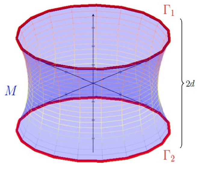
Figure 1 | Graph of M, a catenoid, with boundary curves, Γ₁ and Γ₂, each unit circles separated by a total distance of 2d.

We want to find a minimal surface such that . Let us also assume that M is rotationally symmetric. A simple argument can be made that M must be rotationally symmetric because the boundary conditions are symmetric; if a solution for M were not rotationally symmetric, then there must exist an infinite number of solutions identical to M (but rotated slightly) that are also area-minimizing. However, this violates uniqueness; see⁸^,⁹ for more. Thus, we may locally parametrize M as

Thus, we may locally parametrize M as

$\begin{equation*} F(\theta,z) = (f(z)\cos(\theta), f(z)\sin(\theta), z) \hspace{3em} \text{(4.1)} \end{equation*}$

for some strictly positive $f:\mathbb{R}\rightarrow\mathbb{R}$ with $z\in[-d,d]$ and $\theta\in[0,2\pi]$ . Therefore, our objective is to solve for $f(z)$ .

First, we compute the first fundamental form $g$ of $M$ .

$\frac{\partial F}{\partial z} = (f'(z)\cos(\theta), f'(z)\sin(\theta), 1)$

$\frac{\partial F}{\partial \theta} = (-f(z)\sin(\theta), f(z)\cos(\theta), 0)$

Thus, by Definition (2.4), the first fundamental form is given as

$\begin{equation*} g = \begin{bmatrix} f^2(z) & 0 \\ 0 & 1+(f'(z))^2 \end{bmatrix} \hspace{3em} \text{(4.2)} \end{equation*}$

Further, we can also compute the Gauss map and second fundamental form for M.

$\begin{align*} \frac{\partial F}{\partial z} \times \frac{\partial F}{\partial \theta} &= (-f(z)\cos(\theta), -f(z)\sin(\theta), f(z)f'(z)) \\ \frac{\partial^2 F}{\partial z \partial z} &= (f''(z)\cos(\theta), f''(z)\sin(\theta), 0) \\ \frac{\partial^2 F}{\partial z \partial \theta} &= (-f'(z)\sin(\theta), f'(z)\cos(\theta), 0) \\ \frac{\partial^2 F}{\partial \theta \partial \theta} &= (-f(z)\cos(\theta), -f(z)\sin(\theta), 0) \end{align*}$

So, by Definition (2.5), we have

$\begin{equation*} N = \frac{\frac{\partial F}{\partial z} \times \frac{\partial F}{\partial \theta}}{\left \mid \frac{\partial F}{\partial z} \times \frac{\partial F}{\partial \theta} \right \mid} = \left(\cos(\theta), \sin(\theta), -\frac{f'(z)}{\sqrt{1+(f'(z))^2}}\right) \hspace{3em} \text{(4.3)} \end{equation*}$

where the global (due to assumed orientability) direction of $N$ is of the form $\nu_+$ in equation (2.1). Furthermore, by Definition (2.7), we also find

$\begin{equation*} h = \frac{1}{\sqrt{1+(f'(z))^2}} \begin{bmatrix} -f(z) & 0 \\ 0 & f''(z) \end{bmatrix} \hspace{3em} \text{(4.4)} \end{equation*}$

Thus, by Definition (2.8), we compute S as

$\begin{align*} S = g^{-1}h &= \begin{bmatrix} \frac{1}{f^2(z)} & 0 \\ 0 & \frac{1}{1+(f'(z))^2} \end{bmatrix} \\ &\frac{1}{\sqrt{1+(f'(z))^2}} \begin{bmatrix} -f(z) & 0 \\ 0 & f''(z) \end{bmatrix} \nonumber \\ &= \frac{1}{\sqrt{1+(f'(z))^2}} \begin{bmatrix} -\frac{1}{f(z)} & 0 \\ 0 & \frac{f''(z)}{1+(f'(z))^2} \end{bmatrix} \hspace{3em} \text{(4.5)} \end{align*}$

As such, by Definition (2.9), the mean curvature of M is

$\begin{equation*} H =\frac{1}{2} \text{tr}(S) = \frac{1}{2\sqrt{1+(f'(z))^2}} \left( -\frac{1}{f(z)} + \frac{f''(z)}{\frac{1}{2}+(f'(z))^2} \right) \hspace{1em} \text{(4.6)} \end{equation*}$

Therefore, by Theorem (3.1), the Minimal Surface Equation for M is given by

( $***$ ) $\begin{equation*} \frac{f''(z)}{1+(f'(z))^2} = \frac{1}{f(z)} \end{equation*}$

where $f(-d)=f(d)=1$ . To find a solution $f(z)$ for ( $***$ ), let

$q(z) = \frac{f(z)}{\sqrt{1+(f'(z))^2}}$

Then, we have

$\begin{align*} q'(z) &= \frac{f'(z)}{\sqrt{1+(f'(z))^2}} - \frac{f(z)f'(z)f''(z)}{(1+(f'(z))^2)^{3/2}} \nonumber \\ &= \frac{f'(z)}{\sqrt{1+(f'(z))^2}} \left( 1 - \frac{f(z)f''(z)}{1+(f'(z))^2} \right) \nonumber \\ &= 0 \hspace{3em} \text{(4.7)} \end{align*}$

by ( $***$ ). However, equation (4.7) implies that $q(z)=C$ , for some constant $C$ . Thus, we can solve for $f(z)$ .

$\begin{align*} &\Rightarrow \frac{f(z)}{\sqrt{1+(f'(z))^2}} = C \nonumber \\ &\Rightarrow \frac{f^2(z)}{C^2} = 1 + (f'(z))^2 \nonumber \\ &\Rightarrow \frac{df}{dz} = \sqrt{\frac{f^2(z)}{C^2} - 1} \nonumber \\ &\Rightarrow \int \frac{df}{\sqrt{f^2 - C^2}} = \int \frac{dz}{C} \nonumber \\ &\therefore f(z) = C\cosh\left(\frac{z-z_0}{C}\right) \hspace{3em} \text{(4.8)} \end{align*}$

for some integration constant $z_0$ . However, since M is symmetric about $z = 0$ , we note that $z_0 = 0$ . This fact follows directly from the boundary conditions, $f(-d)=f(d)=1$ , so $z - z_0 = z + z_0$ by the symmetry of the hyperbolic cosine function. Thus, we simplify equation (4.8) and conclude

$\begin{equation*} f(z) = C\cosh\left(\frac{z}{C}\right) \hspace{3em} \text{(4.9)} \end{equation*}$

Finally, we must find the value of C in equation (4.9) given that $f(\pm d)=1$ . Furthermore, according to equation (4.9), C must be the minimum value of $f(z)$ , attained at $z = 0$ . This fact is because $\cosh(u)\geq 1$ for all $u$ . Accordingly, we are brought to the definition of a catenoid.

Definition 4.1 (Catenoid). A catenoid is the unique, non-planar minimal surface of revolution in $\mathbb{R}^3$ given by the local parametrization

$F(u,v) = (a\cosh(v/a)\cos(u), a\cosh(v/a)\sin(u), v)$

for some real $a>0$ . This is equivalent to the initial conditions of two equiradial disks in Plateau’s Problem at the start of this section.

Note that in Definition (4.1), $a=C$ , where $1=C\cosh(d/C)$ , according to the boundary conditions. As such, define

$\begin{equation*} \varphi_d(C) = C\cosh\left(\frac{d}{C}\right) \hspace{3em} \text{(4.10)} \end{equation*}$

Thus, a connected solution $M$ only exists if $\varphi_d(C)=1$ has a positive root. Observe, however, that as $C\rightarrow 0^+$ , we have $\varphi_d(C)\rightarrow\infty$ . Furthermore, as $C\rightarrow\infty$ , we also have $\varphi_d(C)\rightarrow\infty$ . Thus, we know $\varphi_d(C)$ attains a global minimum when $\varphi_d'(C)=0$ . $\varphi_d(C)$ cannot have any local extrema because the hyperbolic cosine function is strictly concave everywhere; that is, since $\varphi_d''(C) > 0$ everywhere, no local extrema (maxima) can occur, and so the only extrema is the global minimum.

This fact leads us to suspect that for certain separation distances between $\Gamma_1$ and $\Gamma_2$ , $\min(\varphi_d(C))>1$ , and there will consequently be no solutions for $M$ . To demonstrate this fact, we must first find the minimum of $\varphi_d(C)$ .

$\begin{equation*} \varphi_d'(C) = \cosh\left(\frac{d}{C}\right) - \frac{d}{C}\sinh\left(\frac{d}{C}\right) = 0 \hspace{3em} \text{(4.11)} \end{equation*}$

$\Rightarrow \cosh\left(\frac{d}{C}\right) = \frac{d}{C}\sinh\left(\frac{d}{C}\right)$

$\Rightarrow \tanh\left(\frac{d}{C}\right) = \frac{C}{d}$

$\therefore \tanh(s) = \frac{1}{s}$

where $s=\frac{d}{C}$ . Implicitly solving equation (4.11) for $s$ , we arrive at one unique solution $s^*\approx 1.19968$ . Thus, for a given $d$ , we have that $\varphi_d(C)$ attains its minimum when $s=s^*$ .

However, also observe that when $\varphi_d(C)=1$ , then $C<1$ . This is once again because $\cosh(u)\geq 1$ . However, because $d$ is strictly positive, we have $\cosh(d/C)>1$ , so $C<1$ . This fact, of course, conforms with our intuition, as $C$ is the minimal radius from $M$ to the $z$ -axis, and as such must be strictly less than the boundary disk radius.

Now that we have $C=\frac{d}{s^*}$ , we substitute into equation (4.10) to find the minimum value of $\varphi_d(C)$ as

$\begin{equation*} \min(\varphi_d(C)) = \frac{d}{s^*}\cosh(s^*) \hspace{3em} \text{(4.12)} \end{equation*}$

Thus, for connected solutions for M to exist, we want $\min(\varphi_d(C))\leq 1$ . Rearranging equation (4.12) to satisfy this inequality, we are left with

$\begin{equation*} d \leq d^* = \frac{s^*}{\cosh(s^*)} \hspace{3em} \text{(4.13)} \end{equation*}$

Consequently, when $d$ becomes too large ( $d>d^*$ ), there are no solutions for the equation $\varphi_d(C)=1$ and thus no connected solutions for $M$ , as we expect. As alluded to in the introduction, this can be seen with real experiments; soap ring bubbles form a catenoid until their separation distance exceeds a certain value, at which point the connecting bubble abruptly pops. See¹⁰^,¹¹ for more.

When $d=d^*$ , one unique solution $C^*$ exists. However, in the case when $d<d^*$ , it is clear that multiple solutions for $\varphi_d(C)$ exist; Figure 2 displays plots of $\varphi_d(C)$ for different values of $d$ . For $d<d^*$ , there are two solutions: $C_1$ and $C_2$ , where $C_2>C^*>C_1$ . Since $C=\min(f(z))$ , we call $C_1$ and $C_2$ the inner and outer-radius catenoid, respectively. Figure 3 displays both catenoids, $M_1$ and $M_2$ , corresponding to $C_1$ and $C_2$ , respectively.

By inspection, we intuitively suspect that $M_2$ has a smaller surface area than $M_1$ ; however, this result must be proven rigorously. As such, we will prove Theorem (4.2), one of the main results of this paper; namely, that when $d<d^*$ the outer-radius catenoid $M_2$ is the solution to Plateau’s Problem for the Dirichlet boundary conditions depicted in Figure 1, while the inner-radius catenoid $M_1$ is not.

Second Variation of Area.

Lemma 4.1. It should be stated that this Lemma is known as Weingarten’s Formula. For additional proof, see⁷. Let $M\subseteq\mathbb{R}^3$ be a regular surface with local parametrization $F(u_1,u_2)$ , first fundamental form $g=[g_{ij}]$ , second fundamental form $h=[h_{ij}]$ , shape operator $S=[S_{ij}]$ , and Gauss map $N$ . Then,

$\frac{\partial N}{\partial u_i} = -\sum_{j=1}^2 S_{ij}\frac{\partial F}{\partial u_j}$

Proof. Since $\langle N,N \rangle = 1$ , it follows that $\partial_i N\in T_pM$ . Thus, we can write

$\begin{equation*} \frac{\partial N}{\partial u_i} = \sum_{k=1}^2 a_{ik}\frac{\partial F}{\partial u_k} \hspace{3em} \text{(4.14)}\end{equation*}$

for some coefficients $a_{ik}$ . Furthermore, we differentiate $\langle N,\partial_j F \rangle=0$ with respect to $u_i$ to find

$\begin{equation*} 0 = \frac{\partial}{\partial u_i} \left\langle N,\frac{\partial F}{\partial u_j} \right\rangle = \left\langle \frac{\partial N}{\partial u_i},\frac{\partial F}{\partial u_j} \right\rangle + \left\langle N,\frac{\partial^2 F}{\partial u_i \partial u_j} \right\rangle \hspace{3em} \text{(4.15)}\end{equation*}$

However, since $h_{ij}=\left\langle N,\partial_{ij}F \right\rangle$ by Definition (2.7), we simplify equation (4.15) and have

$\begin{equation*} \left\langle \frac{\partial N}{\partial u_i},\frac{\partial F}{\partial u_j} \right\rangle = -h_{ij}\hspace{3em} \text{(4.16)} \end{equation*}$

But using equation (4.14), we also have

$\begin{equation*} \left\langle \frac{\partial N}{\partial u_i},\frac{\partial F}{\partial u_j} \right\rangle = \sum_{k=1}^2 a_{ik} \left\langle \frac{\partial F}{\partial u_k},\frac{\partial F}{\partial u_j} \right\rangle = \sum_{k=1}^2 a_{ik}g_{jk} \hspace{3em} \text{(4.17)} \end{equation*}$

because $g_{jk}=\langle \partial_j F,\partial_k F \rangle$ , by Definition (2.4). Thus, we compare $\langle \partial_i N,\partial_j F \rangle$ in equations (4.16) and (4.17) and conclude

$\begin{equation*} \sum_{k=1}^2 a_{ik}g_{jk} = -h_{ij} \hspace{3em} \text{(4.18)} \end{equation*}$

However, with respect to the coordinate basis $\{\partial_1 F, \partial_2 F\}$ , equation (4.18) expands to the matrix equation

$\begin{equation*} g\begin{bmatrix} a_{i1} \\ a_{i2} \end{bmatrix} = -\begin{bmatrix} h_{i1} \\ h_{i2} \end{bmatrix} \hspace{3em} \text{(4.19)} \end{equation*}$

$\begin{equation*} \therefore \begin{bmatrix} a_{i1} \\ a_{i2} \end{bmatrix} = -g^{-1}\begin{bmatrix} h_{i1} \\ h_{i2} \end{bmatrix} \hspace{3em} \text{(4.20)} \end{equation*}$

for $j = 1, 2$ . By definition, equation (4.20) implies

$\begin{equation*} a_{ik} = -g^{-1}h_{ik} = -S_{ik} \hspace{3em} \text{(4.21)} \end{equation*}$

Thus, plugging equation (4.21) into equation (4.14), we get our desired result.

Lemma 4.2. Let $M(s)\subseteq\mathbb{R}^3$ be a family of regular surfaces with local parametrizations in the form of equation (3.1), first fundamental form $g(s)$ , and shape operator $S$ , such that $M(0)=M$ . Then,

(a) $\text{tr}(g(0)^{-1}g'(0)) = -2\varphi H = 0$

(b) $\text{tr}(g(0)^{-1}g''(0)) = 2 \mid \nabla_M\varphi \mid ^2 - 2\text{tr}(S^2)\varphi^2$

where $\mid \nabla_M\varphi \mid^{2} = \sum_{i,j=1}^2 g^{ij}\frac{\partial\varphi}{\partial u_i}\frac{\partial\varphi}{\partial u_j}$ is the surface gradient of $\varphi$ for smooth $\varphi:M\rightarrow\mathbb{R}$ .

Proof. Since $g(0)^{-1}g'(0) = -2\varphi H$ from equation (3.6), the result for (a) trivially follows. As for (b), first consider $g'(s)_{ij}$ . By equation (3.5), we have

$g'(s)_{ij} = \left\langle \frac{\partial V}{\partial u_i},\frac{\partial \stackrel{\sim}F}{\partial u_j} \right\rangle + \left\langle \frac{\partial \stackrel{\sim}F}{\partial u_i},\frac{\partial V}{\partial u_j} \right\rangle$

for $V(u_1,u_2)=\varphi(u_1,u_2)N(u_1,u_2)$ . Therefore, we compute $g''(s)_{ij}$ as

$\begin{align*} g''(s)_{ij} &= \left\langle \frac{\partial^2 V}{\partial u_i \partial s},\frac{\partial \stackrel{\sim}{F}}{\partial u_j} \right\rangle + \left\langle \frac{\partial V}{\partial u_i},\frac{\partial^2 \stackrel{\sim}{F}}{\partial u_j \partial s} \right\rangle \nonumber \\ &\quad + \left\langle \frac{\partial^2 \stackrel{\sim}{F}}{\partial u_i \partial s},\frac{\partial V}{\partial u_j} \right\rangle + \left\langle \frac{\partial \stackrel{\sim}{F}}{\partial u_i},\frac{\partial^2 V}{\partial u_j \partial s} \right\rangle \nonumber \\ &= 2 \left\langle \frac{\partial V}{\partial u_i},\frac{\partial V}{\partial u_j} \right\rangle \nonumber \\ &= 2 \left\langle \frac{\partial\varphi}{\partial u_i}N + \varphi\frac{\partial N}{\partial u_i}, \frac{\partial\varphi}{\partial u_j}N + \varphi\frac{\partial N}{\partial u_j} \right\rangle \nonumber \\ &= 2\left(\frac{\partial\varphi}{\partial u_i}\frac{\partial\varphi}{\partial u_j} + \varphi^2 \left\langle\frac{\partial N}{\partial u_i},\frac{\partial N}{\partial u_j}\rangle\right) \nonumber \\ &= 2 \frac{\partial\varphi}{\partial u_i}\frac{\partial\varphi}{\partial u_j} + 2\varphi^2 \sum_{k,l=1}^2 S_{ik}S_{jl}g_{kl} \hspace{3em} \text{(4.22)} \end{align*}$

Thus, from equation (4.22), we conclude

$\begin{align*} \text{tr}(g(0)^{-1}g''(0)) &= 2\sum_{i,j=1}^2 g^{ij}\frac{\partial\varphi}{\partial u_i}\frac{\partial\varphi}{\partial u_j} + 2\varphi^2\sum_{i,j,k,l=1}^2 g^{ij}S_{ik}S_{jl}g_{kl} \nonumber \\ &= 2\mid \nabla_M\varphi \mid^2 + 2\text{tr}(S^2)\varphi^2 \hspace{5em} \text{(4.23)} \end{align*}$

as desired. Note that sign conventions depending on metric signature might flip $S^2$ trace sign in some contexts, but follows derivation above.

For a minimal surface M to be the solution to Plateau’s Problem, we must confirm that M is indeed area-minimizing while satisfying the Minimal Surface Equation; this implies that the area of M would satisfy the “second derivative test.” As such, we are brought to the definition of the Second Variation of Area.

Theorem 4.1 (Second Variation of Area). Let $M(s)\subseteq\mathbb{R}^3$ be a family of regular surfaces with local parametrizations in the form of equation (3.1), first fundamental form $g(s)$ , and shape operator $S$ , such that $M(0)=M$ , where $M$ is a minimal surface. Then, the Second Variation of Area of $M$ is given as

$\begin{equation*} \frac{d^2}{ds^2} \text{Area}(M(s)) \Big|_{s=0}= \iint_M \left( \mid \nabla_M\varphi \mid ^{2} - \text{tr}(S^2)\varphi^2 \right) \sqrt{\det(g)} \, du_1 du_2 \end{equation*}$

for all smooth $\varphi:M\rightarrow\mathbb{R}$ such that $\varphi=0$ on $\partial M$ .

Remark 4.1. A minimal surface $M\subseteq\mathbb{R}^3$ is locally minimizing if

$\iint_M \left( \mid \nabla_M\varphi \mid^{2} - \text{tr}(S^2)\varphi^2 \right) \sqrt{\det(g)} \, du_1 du_2 > 0$

for all $\varphi:M\rightarrow\mathbb{R}$ with $\varphi=0$ on $\partial M$ . This is the second derivative test for the area of M.

Proof. From ( $*$ ), we find

$\begin{equation*} \frac{d^2}{ds^2}\text{Area}(M(s)) \Big|_{s=0} = \iint_M \frac{\partial^2}{\partial s^2}\sqrt{\det(g(s))}\Big|_{s=0} \, du_1 du_2 \hspace{3em} \text{(4.24)} \end{equation*}$

Thus, we must find $\partial_s^2\sqrt{\det(g)}$ . Recall from equation (3.4) that we have

$\frac{\partial}{\partial s}\sqrt{\det(g(s))} = \frac{1}{2}\sqrt{\det(g(s))}\text{tr}(g(s)^{-1}g'(s))$

$\begin{align*} \Rightarrow \frac{\partial^2}{\partial s^2}\sqrt{\det(g(s))} &= \frac{1}{4}\sqrt{\det(g(s))}\operatorname{tr}^2(g(s)^{-1}g'(s)) \nonumber \\ & \quad + \frac{1}{2}\sqrt{\det(g(s))} \nonumber \\ & \quad \times \Bigl( -\operatorname{tr}(g(s)^{-1}g'(s)g(s)^{-1}g'(s)) \nonumber \\ & \quad + \operatorname{tr}(g(s)^{-1}g''(s)) \Bigr) \hspace{3em} \text{(4.25)} \end{align*}$

This result comes simply from $\partial_s(g(s)^{-1}) = -g(s)^{-1}g'(s)g(s)^{-1}$ .

$\Rightarrow \frac{\partial^2}{\partial s^2}\sqrt{\det(g(s))}\Big|_{s=0} = \frac{1}{2}\sqrt{\det(g(0))}\text{tr}(g(0)^{-1}g''(0))$

because $\text{tr}(g(0)^{-1}g'(0)) = 0$ since $M(0)$ is a minimal surface. Finally, we substitute Lemmas (4.2, a) and (4.2, b) into equation 4.25 and obtain our desired result.

Now, we will prove the main result of this section, Theorem (4.2).

Outer-Radius Catenoid Stability

Theorem 4.2 (Outer-Radius Catenoid Stability). Consider Plateau’s Problem for the boundary curves $\Gamma_{1,2}$ consisting of two coaxial unit discs in $\mathbb{R}^3$ , as seen in Figure 1, such that $\Gamma_{1,2} = \{(x,y,z) | x^2+y^2=1, z=\pm d\}$ for $d<d^*$ , where $d^*$ is defined in equation (4.13). Consequently, there exist two catenoids $M_1\subseteq\mathbb{R}^3$ and $M_2\subseteq\mathbb{R}^3$ such that $\partial M_{1,2}=\Gamma_1\cup\Gamma_2$ , and $\min M_2=C_2 > \min M_1=C_1$ . Then, $M_2$ is stable, while $M_1$ is unstable; i.e. $M_2$ is the unique solution to Plateau’s Problem.

Proof. We present a self-contained proof of Theorem (4.2). However, for a more concise proof using Sturm-Liouville theory, see¹². We will start by proving that Area( $M_2$ ) < Area( $M_1$ ) and then prove that $M_2$ is indeed the unique solution to Plateau’s Problem by using Theorem (4.1).

First, note that $M_{1,2}$ is parametrized by equation (4.1), where

$\begin{equation*} f(z) = C_{1,2}\cosh\left(\frac{z}{C_{1,2}}\right) \hspace{3em} \text{(4.26)} \end{equation*}$

from equation (4.9). Further, by equation (4.2), the first fundamental form for $M_{1,2}$ is given by

$\begin{equation*} g_{1,2} = \begin{bmatrix} C_{1,2}^2\cosh^2\left(\frac{z}{C_{1,2}}\right) & 0 \\ 0 & \cosh^2\left(\frac{z}{C_{1,2}}\right) \end{bmatrix} \hspace{3em} \text{(4.27)} \end{equation*}$

and its inverse as

$\begin{equation*} g_{1,2}^{-1} = \begin{bmatrix} \frac{1}{C_{1,2}^2\cosh^2(z/C_{1,2})} & 0 \\ 0 & \frac{1}{\cosh^2(z/C_{1,2})} \end{bmatrix} \hspace{3em} \text{(4.28)} \end{equation*}$

Therefore, we also have

$\begin{equation*} \sqrt{\det(g_{1,2})} = C_{1,2}\cosh^2\left(\frac{z}{C_{1,2}}\right) \hspace{3em} \text{(4.29)} \end{equation*}$

and

$\begin{equation*} S = \begin{bmatrix} \frac{1}{\cosh(z/C_{1,2})} & 0 \\ 0 & \frac{1}{C_{1,2}\cosh(z/C_{1,2})} \end{bmatrix} \hspace{3em} \text{(4.30)} \end{equation*}$

by equation (4.5). Thus, we compute

$\begin{equation*} \text{tr}(S^2) = \frac{2}{C_{1,2}^2\cosh^4(z/C_{1,2})} \hspace{3em} \text{(4.31)} \end{equation*}$

Now, by Remark (2.4), we calculate Area( $M_{1,2}$ ) as

$\begin{align*} \text{Area}(M_{1,2}) &= \iint_M \sqrt{\det(g_{1,2})} \, d\theta dz \nonumber \\ &= \int_{-d}^d \int_0^{2\pi} C_{1,2}\cosh^2\left(\frac{z}{C_{1,2}}\right) \, d\theta dz \nonumber \\ &= 2\pi C_{1,2} \int_{-d}^d \left( \frac{1}{2} + \frac{1}{2}\cosh\left(\frac{2z}{C_{1,2}}\right) \right) \, dz \nonumber \\ &= 2\pi C_{1,2} d + \pi C_{1,2}^2 \sinh\left(\frac{2d}{C_{1,2}}\right) \hspace{3em} \text{(4.32)} \end{align*}$

Define $s_{1,2}=\frac{d}{C_{1,2}}$ and function $\zeta(x):\mathbb{R}\rightarrow\mathbb{R}$ such that

$\begin{equation*} \zeta(x) = xd + \frac{x^2}{2}\sinh\left(\frac{2d}{x}\right) \hspace{3em} \text{(4.33)} \end{equation*}$

According to equation (4.10, we must have that

$\begin{equation*} C_{1,2} = \text{sech}\left(\frac{d}{C_{1,2}}\right) = \text{sech}(s_{1,2}) \hspace{3em} \text{(4.34)} \end{equation*}$

and consequently

$\begin{equation*} d = s_{1,2}\text{sech}(s_{1,2}) \hspace{3em} \text{(4.35)} \end{equation*}$

These two equalities are because $\varphi_d(C_{1,2})=1$ in equation (4.10). Therefore, we simplify $\zeta(C_{1,2})$ as

$\begin{align*} \zeta(C_{1,2}) &= dC_{1,2} + C_{1,2}^2\sinh\left(\frac{d}{C_{1,2}}\right)\cosh\left(\frac{d}{C_{1,2}}\right) \nonumber \\ &= d\text{sech}(s_{1,2}) + \tanh\left(\frac{d}{C_{1,2}}\right) \nonumber \\ &= \frac{s_{1,2}}{\cosh^2(s_{1,2})} + \tanh(s_{1,2}) \hspace{3em} \text{(4.36)} \end{align*}$

by equations (4.34) and (4.35). Define a function $\Phi(u(d)):\mathbb{R}\rightarrow\mathbb{R}$ such that

$\begin{equation*} \Phi(u(d)) = \frac{u}{\cosh^2(u)} + \tanh(u) \hspace{3em} \text{(4.37)} \end{equation*}$

where

$\begin{equation*} u\text{sech}(u) = d \hspace{3em} \text{(4.38)} \end{equation*}$

according to equation (4.35). Also note that equation (4.38) implies that

$\begin{equation*} \frac{\partial u}{\partial d} = \frac{1}{\text{sech}(u)(1-u\tanh(u))} \end{equation*}$

4.39

Thus, we find $\Phi'(u(d))$ as

$\begin{align*} \frac{\partial\Phi}{\partial d} &= \frac{\partial\Phi}{\partial u}\frac{\partial u}{\partial d} \nonumber \\ &= \frac{2\text{sech}^2(u)(1-u\tanh(u))}{\text{sech}(u)(1-u\tanh(u))} \nonumber \\ &= 2\text{sech}(u) \hspace{3em} \text{(4.40)} \end{align*}$

Hence, from equations (4.36) and (4.40), we have that $\partial_d \zeta(C_{1,2}) = 2\text{sech}(s_{1,2})$ . This implies that

$\begin{equation*} \frac{\partial}{\partial d}(\zeta(C_1) - \zeta(C_2)) = 2(\text{sech}(s_1) - \text{sech}(s_2)) < 0 \hspace{3em} \text{(4.41)} \end{equation*}$

since $s_1 \propto C_1^{-1} > s_2 \propto C_2^{-1}$ , where $C_2>C_1$ . However, equation (4.41) implies that the difference between $\zeta(C_1)$ and $\zeta(C_2)$ , denoted as $D_\zeta(d)$ , is strictly decreasing as $d$ increases. As such, we bound this difference by considering the endpoints in the interval $d\in(0,d^*)$ . Note that in equation (4.38), the maximum value of $u\text{sech}(u)$ occurs when $u=s^*$ and thus when $d=d^*$ . Therefore, at $d=d^*$ , we have that $s_1=s_2$ and hence $D_\zeta(d^*)=0$ . However, in our interval for $d$ , we have $d<d^*$ , and so $D_\zeta(d)>0$ by equation (4.41). As $d$ increases, $D_\zeta(d)$ decreases, so by the converse, as $d$ decreases, $D_\zeta(d)$ increases. Thus, we conclude that $\zeta(C_1) > \zeta(C_2)$ . However, by equation (4.32), we also note

$\begin{equation*} \text{Area}(M_1) > \text{Area}(M_2) \hspace{3em} \text{(4.42)} \end{equation*}$

By equation (4.42), it therefore suffices to show that if $M_2$ is area-minimizing, it then must be the unique solution to Plateau’s Problem.

Let $R=C_2$ and $M=M_2$ . Now consider the Second Variation of Area for $M(0)=M$ . Let $\varphi=\varphi(z):M\rightarrow\mathbb{R}$ be a variational function such that $\varphi(\pm d)=0$ and $\partial_\theta\varphi=0$ . That is, we only consider axisymmetric variations and not rotational ones; this restriction is necessary, as rotational variations will not distinguish stability between the catenoids. We define a $\varphi(z)$ instead of $\varphi(\theta, z)$ since M is rotationally symmetrical and surface perturbations will therefore be independent of $\theta$ . Furthermore, non-axisymmetrical perturbations will result in apparent stability for both catenoids, which is unfavorable for our proof¹³.

By Theorem (4.1), we therefore have

$\begin{align*} \frac{d^2}{ds^2}&\operatorname{Area}(M(s)) \Big|_{s=0} \nonumber \\ &= \iint_M \left( \sum_{i,j=1}^2 g^{ij}\frac{\partial\varphi}{\partial u_i}\frac{\partial\varphi}{\partial u_j} - \operatorname{tr}(S^2)\varphi^2 \right) \sqrt{\det(g)} \, du_1 du_2 \nonumber \\ &= \int_{-d}^d \int_0^{2\pi} \left( \frac{1}{\cosh^2(z/R)}\left(\frac{\partial\varphi}{\partial z}\right)^2 - \frac{2\varphi^2}{R^2\cosh^4(z/R)} \right) \nonumber \\ & \quad \times R\cosh^2(z/R) \, d\theta dz \nonumber \\ &= 2\pi R \int_{-d}^d \left( \left(\frac{\partial\varphi}{\partial z}\right)^2 - \frac{2\varphi^2}{R^2\cosh^2(z/R)} \right) \, dz \nonumber \\ &= 2\pi R \int_{-d}^d \varphi \left( -\frac{d^2\varphi}{dz^2} - \frac{2}{R^2\cosh^2(z/R)}\varphi \right) \, dz \nonumber \\ &= 2\pi R \int_{-d}^d \varphi L\varphi \, dz \end{align*}$

(4.43)

where $L\varphi$ is defined as

$\begin{equation*} L\varphi = -\frac{d^2\varphi}{dz^2} - \frac{2}{R^2\cosh^2(z/R)}\varphi \end{equation*}$

(4.44)

In a similar manner to earlier, define $s^* > s = \frac{d}{R}$ . Now, consider the function

$\begin{equation*} h(z) = 1 - \frac{z}{R}\tanh\left(\frac{z}{R}\right) \end{equation*}$

(4.45)

Then we find the derivatives of $h(z)$ as

$\begin{equation*} \frac{dh}{dz} = -\frac{1}{R}\tanh\left(\frac{z}{R}\right) - \frac{z}{R^2\cosh^2(z/R)}\end{equation*}$

(4.46)

$\begin{align*} \frac{d^2h}{dz^2} &= -\frac{2}{R^2\cosh^2(z/R)} + \frac{2z}{R^3\cosh^2(z/R)}\tanh\left(\frac{z}{R}\right) \nonumber \\ &= -\frac{2}{R^2\cosh^2(z/R)}\left( 1 - \frac{z}{R}\tanh\left(\frac{z}{R}\right) \right) \nonumber \\ &= -\frac{2}{R^2\cosh^2(z/R)}h(z) \end{align*}$

(4.47)

Observe now that equation (4.47) implies that $Lh(z)=0$ . Furthermore, on the interval $z\in[-d,d]$ , the function $h(z)$ is strictly positive. This is because $\partial_z g(z) = \frac{z}{R}\tanh(z/R) > 0$ for all $z$ , and thus $g(z)=1$ at the unique solution $z=s^*$ . However, since $R>C^*$ , we have $\frac{d}{R}<s^*$ , so $g(z)<1$ for all $z\in[-d,d]$ (since $h(-z)=h(z)$ ). This implies that $h(z)>0$ . Thus, for some continuous function $f(z)$ such that $f(\pm d) = 0$ , define

$\begin{equation*} \varphi(z) = f(z)h(z) \end{equation*}$

(4.48)

Then, by equation (4.44), consider

$\begin{align*} \varphi(z)L\varphi(z) &= f(z)h(z) \left( -\varphi''(z) - \frac{2}{R^2\cosh^2(z/R)}\varphi(z) \right) \nonumber \\ &= f(z)h(z) \Bigl( -f''(z)h(z) - 2f'(z)h'(z) \nonumber \\ & \quad - f(z)h''(z) - \frac{2f(z)h(z)}{R^2\cosh^2(z/R)} \Bigr) \nonumber \\ &= f''(z)f(z)h^2(z) - 2f(z)h(z)f'(z)h'(z) \nonumber \\ &\quad + f(z)h(z)Lh(z)_{0} \nonumber \\ &= -f''(z)f(z)h^2(z) - 2f(z)h(z)f'(z)h'(z) \hspace{3em} \text{(4.49)} \end{align*}$

Now we substitute equation (4.49) into equation (4.43).

$\begin{align*} \int_{-d}^d \varphi L\varphi \, dz &= \int_{-d}^d -f''(z)f(z)h^2(z) \, dz \nonumber \\ &\quad - \int_{-d}^d 2f(z)h(z)f'(z)h'(z) \, dz \nonumber \\ &= \int_{-d}^d -f''(z)f(z)h^2(z) \, dz \nonumber \\ &\quad + \int_{-d}^d h^2(z)\left( (f'(z))^2 + f(z)f''(z) \right) \, dz \nonumber \\ &= \int_{-d}^d h^2(z)(f'(z))^2 \, dz \nonumber \\ &= \int_{-d}^d h^2(z)\left(\frac{d}{dz}\left(\frac{\varphi(z)}{h(z)}\right)\right)^2 \, dz \hspace{3em} \text{(4.50)} \end{align*}$

Here we used integration by parts on $d(h^2(z))$ . Therefore, by equation (4.50), we conclude that

$\begin{equation*} \frac{d^2}{ds^2}\text{Area}(M(s)) \Big|_{s=0} > 0 \hspace{3em} \text{(4.51)} \end{equation*}$

and thus, by Remark (4.1), it follows that M is a solution to Plateau’s Problem. Furthermore, as we have proven in equation (4.42), $M_1$ , while satisfying the Minimal Surface Equation, cannot be a solution. A similar argument made in equation (4.50) cannot be made for $M_1$ ; since $C_1 > C^*$ , the function $h(z)$ has a root and thus $f(z)$ is not a continuous function. Therefore, $M = M_2$ is the unique solution; the outer-radius catenoid is stable and area-minimizing while the inner-radius catenoid is not.

Minimal Graphs

This section will introduce the necessary background into minimal graphs, a specific class of minimal surfaces; furthermore, we will prove the main result of the uniqueness of minimal (planar) graphs. However, we must first introduce the definition of minimal graphs.

Definition 5.1 (Minimal Graph). Let $\Omega\subseteq\mathbb{R}^2$ be a bounded domain. Then, a regular surface $M$ is called a minimal graph if

$M = \{ (x,y,f(x,y))\in\mathbb{R}^3 : (x,y)\in\Omega \}$

is a minimal surface, where $f:\Omega\rightarrow\mathbb{R}$ .

In a similar manner to the Minimal Surface Equation, we desire to find a generalized equation to determine if a regular surface M is a minimal graph; to do so, we must solve the Minimal Surface Equation for M. Let $M\subseteq\mathbb{R}^3$ be a regular surface in the form of Definition (5.1). Then, the local parametrization of M is

$\begin{equation*} F(x,y) = (x,y,f(x,y)) \hspace{3em} \text{(5.1)} \end{equation*}$

Thus, according to Definition (2.4), the first fundamental form of M is given as

$\begin{equation*} g = \begin{bmatrix} 1+f_x^2 & f_x f_y \\ f_x f_y & 1+f_y^2 \end{bmatrix} \hspace{3em} \text{(5.2)} \end{equation*}$

and we also have

$\begin{equation*} \det(g) = (1+f_x^2)(1+f_y^2) - (f_x f_y)^2 = 1+ \mid \nabla f \mid ^{2} \hspace{3em} \text{(5.3)} \end{equation*}$

Therefore, we compute the inverse of g as

$\begin{equation*} g^{-1} = \frac{1}{1+ \mid \nabla f \mid ^{2}} \begin{bmatrix} 1+f_y^2 & -f_x f_y \\ -f_x f_y & 1+f_x^2 \end{bmatrix} \hspace{3em} \text{(5.4)} \end{equation*}$

By Definition (2.5), find the Gauss map N as

$\begin{equation*} N = \frac{\frac{\partial F}{\partial x} \times \frac{\partial F}{\partial y}}{\left \mid \frac{\partial F}{\partial x} \times \frac{\partial F}{\partial y} \right \mid} = \frac{(-f_x, -f_y, 1)}{\sqrt{1+ \mid \nabla f \mid^{2}}} \hspace{5em} \text{(5.5)} \end{equation*}$

and by Definition (2.7), the second fundamental form is then

$\begin{equation*} h = \frac{1}{\sqrt{1+\mid \nabla f \mid^{2}}} \begin{bmatrix} f_{xx} & f_{xy} \\ f_{yx} & f_{yy} \end{bmatrix} \hspace{3em} \text{(5.6)} \end{equation*}$

Therefore, by Definition (2.8), we compute the shape operator as

$\begin{equation*} \begin{aligned} S = \frac{1}{(1+ \mid \nabla f \mid^2)^{3/2}} & \\ \times \begin{bmatrix} (1+f_y^2)f_{xx} - f_x f_y f_{yx} & (1+f_y^2)f_{xy} - f_x f_y f_{yy} \\ -f_x f_y f_{xx} + (1+f_x^2)f_{yx} & -f_x f_y f_{xy} + (1+f_x^2)f_{yy} \end{bmatrix} \end{aligned} \hspace{3em} \text{(5.7)} \end{equation*}$

Finally, by Definition (2.9), the mean curvature is then

$\begin{align*} H &= \frac{(1+f_y^2)f_{xx} - 2f_x f_y f_{xy} + (1+f_x^2)f_{yy}}{2(1+|\nabla f|^2)^{3/2}} \nonumber \\ &= \frac{1}{2}\frac{\partial}{\partial x}\left(\frac{f_x}{\sqrt{1+|\nabla f|^2}}\right) + \frac{1}{2}\frac{\partial}{\partial y}\left(\frac{f_y}{\sqrt{1+|\nabla f|^2}}\right) \nonumber \\ &= \frac{1}{2}\text{div} \left( \frac{\nabla f}{\sqrt{1+|\nabla f|^2}} \right). \hspace{5em} \text{(5.8)} \end{align*}$

Now, by Theorem (3.1), we are motivated to define the Minimal Graph Equation.

Theorem 5.1. For a bounded domain $\Omega\subseteq\mathbb{R}^2$ , a regular surface $M$ in the form of

$M = \{ (x,y,f(x,y))\in\mathbb{R}^3 : (x,y)\in\Omega \}$ is a minimal graph if $\text{div} \left( \frac{\nabla f}{\sqrt{1+\mid \nabla f \mid ^2}} \right) = 0$ for a function $f:\Omega \rightarrow \mathbb{R}$ .

Now that we have the Minimal Graph Equation defined, we will prove the main result of this section; specifically, we will conclude the uniqueness of minimal graphs, in Theorem (5.3), and the uniqueness of planar graphs for boundaries confined in a plane in $\mathbb{R}^3$ , in Corollary (5.1).

First, consider Plateau’s Problem for the following:

Let $\Omega\subseteq\mathbb{R}^2$ be a bounded domain with smooth curve $\Gamma\in\mathbb{R}^3$ above $\partial\Omega$ such that $\Gamma = \{ (x,y,f(x,y)) | f:\partial\Omega\rightarrow\mathbb{R} \}$

Consider then a regular surface $M\subseteq\mathbb{R}^3$ such that $M = \{ (x,y,u(x,y)) | u:\Omega\rightarrow\mathbb{R} \}$

where $\partial M=\Gamma$ . Then, we will prove in Theorem (5.3) that $M$ is unique. However, we will need to first explore the Maximum Principle for linear elliptic equations.

Maximum Principle. Let $\Omega\subseteq\mathbb{R}^2$ be a bounded domain. Define the function $u(x_1,x_2):\Omega\rightarrow\mathbb{R}$ and the linear operator $L$ such that

$\begin{equation*} Lu = \sum_{i,j=1}^2 a_{ij}(x_1,x_2)\frac{\partial^2 u}{\partial x_i \partial x_j} + \sum_{i=1}^2 b_i(x_1,x_2)\frac{\partial u}{\partial x_i} \hspace{3em} \text{(5.11)} \end{equation*}$

where $a_{ij}(x_1,x_2), b_i(x_1,x_2):\Omega\rightarrow\mathbb{R}$ are smooth functions. Then, $L$ is called elliptic if the symmetric matrix

$\begin{equation*} A(x_1,x_2) = \begin{bmatrix} a_{11}(x_1,x_2) & a_{12}(x_1,x_2) \\ a_{21}(x_1,x_2) & a_{22}(x_1,x_2) \end{bmatrix} > 0 \hspace{3em} \text{(5.12)} \end{equation*}$

for all $(x_1,x_2)\in\Omega$ . $A(x_1,x_2)$ is positive definite; i.e., $\langle v, A v \rangle > 0$ $\forall v \in \mathbb{R}^2$ . When we have $Lu=0$ , we have an elliptic equation, and thus we can apply the Maximum Principle.

Theorem 5.2 (Maximum Principle). Note here that Theorem (5.2) is actually the weak Maximum Principle; for a proof of the strong version with a generalization to $\mathbb{R}^n$ , see¹⁴. Let $\Omega\subseteq\mathbb{R}^2$ be a bounded domain with the smooth function $u(x_1,x_2):\Omega\rightarrow\mathbb{R}$ and operator $L$ as defined in equation (5.11). Then, if $Lu=0$ , we have

$\max_\Omega u = \max_{\partial\Omega} u \quad\text{and}\quad \min_\Omega u = \min_{\partial\Omega} u$

Proof. The following proof is adapted from Colding and Minicozzi¹⁵. We prove this by contradiction. Suppose a function $\varphi(x_1,x_2):\Omega\rightarrow\mathbb{R}$ reaches a global maximum inside $\Omega$ ; i.e., there exists a $x_0\in\Omega\setminus\partial\Omega$ such that $\varphi(x_0)$ attains a maximum. Then, by the first derivative test, we have $\nabla\varphi(x_0)=0$ . Furthermore, by the second derivative text, we also have

$\begin{equation*} D^2\varphi(x_0) \leq 0 \hspace{3em} \text{(5.13)} \end{equation*}$

where $D^2$ denotes the Hessian matrix. Therefore, we find

$\begin{equation*} \sum_{i,j=1}^2 a_{ij}(x_1,x_2)\frac{\partial^2\varphi}{\partial x_i \partial x_j}(x_0) = \text{tr}(A\cdot D^2\varphi(x_0)) \leq 0 \hspace{3em} \text{(5.14)} \end{equation*}$

where $A=[a_{ij}(x_1,x_2)]$ is defined in equation (5.12). In general, if we have an $n \times n$ symmetric positive definite matrix A and negative semidefinite matrix B, we have that tr(AB) $\leq$ 0. The proof for this comes simply when we define a matrix $C = A^{1/2} B A^{1/2}$ and consider the definiteness of C, where $v^T C v \leq 0$ for all $v \in \mathbb{R}^n$ . Thus, from equation (5.11), we have

$\begin{equation*} L\varphi(x_0) = \text{tr}(A\cdot D^2\varphi(x_0)) + \sum_{i=1}^2 b_i\frac{\partial\varphi}{\partial x_i}(x_0) \leq 0 \hspace{3em} \text{(5.15)} \end{equation*}$

Now consider a function $u(x_1,x_2):\Omega\rightarrow\mathbb{R}$ such that $Lu=0$ . Define

$\begin{equation*} u_\epsilon(x_1,x_2) = u(x_1,x_2) + \epsilon e^{\gamma x_1} \hspace{3em} \text{(5.16)} \end{equation*}$

where $\epsilon>0$ and $\gamma>0$ are arbitrary real numbers. Then, suppose that $u_\epsilon$ attains a maximum at $x_0\in\Omega\setminus\partial\Omega$ . Then, by equation (5.15), we find

$\begin{equation*} Lu_\epsilon(x_0) \leq 0 \hspace{3em} \text{(5.17)} \end{equation*}$

However, we want to show that $Lu_\epsilon>0$ to arise at a contradiction; also consider

$\begin{align*} Lu_\epsilon &= {Lu}_{0} + \epsilon Le^{\gamma x_1} \nonumber \\ &= \epsilon\sum_{i,j=1}^2 a_{ij}\frac{\partial^2 e^{\gamma x_1}}{\partial x_i \partial x_j} + \epsilon\sum_{i=1}^2 b_i\frac{\partial e^{\gamma x_1}}{\partial x_i} \nonumber \\ &= \epsilon a_{11}\gamma^2 e^{\gamma x_1} + \epsilon b_1\gamma e^{\gamma x_1} \nonumber \\ &= \epsilon\gamma e^{\gamma x_1}(a_{11}\gamma + b_1) \nonumber \\ &\geq \epsilon\gamma e^{\gamma x_1}(a_{11}\gamma - \max_\Omega|b_1|) \hspace{3em} \text{(5.18)} \end{align*}$

However, we also have

$\begin{equation*} a_{11} = \begin{bmatrix} 1 & 0 \end{bmatrix} A \begin{bmatrix} 1 \\ 0 \end{bmatrix} \geq \theta > 0 \hspace{3em} \text{(5.19)} \end{equation*}$

for some $\theta > 0$ , since A is positive definite. Therefore, we use equation (5.19) and rewrite equation (5.18) as

$\begin{equation*} Lu_\epsilon \geq \epsilon\gamma e^{\gamma x_1}(\theta\gamma - \max_\Omega|b_1|) \hspace{3em} \text{(5.20)} \end{equation*}$

Now, choose $\gamma$ such that

$\begin{equation*} \gamma > \frac{\max_\Omega|b_1|}{\theta} > 0 \hspace{3em} \text{(5.21)} \end{equation*}$

so equation (5.20) becomes

$\begin{equation*} Lu_\epsilon > 0 \hspace{3em} \text{(5.22)} \end{equation*}$

However, we compare equations (5.22) and (5.17) and arise at a contradiction! As such, we conclude

$\begin{equation*} \max_\Omega u_\epsilon = \max_{\partial\Omega} u_\epsilon \hspace{3em} \text{(5.23)} \end{equation*}$

However, also note that as $\epsilon \rightarrow 0$ in equation (5.23), we arrive at

$\begin{equation*} \max_\Omega u = \max_{\partial\Omega} u \hspace{3em} \text{(5.24)} \end{equation*}$

as desired. To prove the same argument for the minimum, we instead choose $u_\epsilon=u-\epsilon e^{\gamma x_1}$ . Also, then, note that $D^2 u_\epsilon(x_0)\geq 0$ , so we have $Lu_\epsilon\geq 0$ . However, we then have $Lu_\epsilon=-\epsilon Le^{\gamma x_1}$ , which must then be strictly negative according to equation (5.22). Thus, we arrive at a contradiction and the result follows. For a more detailed proof, see¹⁶^,¹⁷.

Uniqueness of Minimal Graphs

Lemma 5.1. Let the functions $u(x,y)$ and $v(x,y)$ satisfy the Minimal Graph Equation, with the function $w(x,y):=u(x,y)-v(x,y)$ . Then,

$\text{div}(A\nabla w) = 0$

for some symmetric matrix $A$ in the form of equation (5.12).

Proof. Define a map $F:\mathbb{R}^2\rightarrow\mathbb{R}^2$ such that

$\begin{equation*} F(x) = \frac{x}{\sqrt{1+|x|^2}} \hspace{3em} \text{(5.25)} \end{equation*}$

Then, since $u$ and $v$ are both minimal surfaces, we therefore have that $\text{div}(F(\nabla u)) = \text{div}(F(\nabla v)) = 0$ . Now, consider

$\begin{align*} F(\nabla u) - F(\nabla v) &= \int_0^1 \frac{d}{dt} F(\nabla v + t(\nabla u - \nabla v)) \, dt \nonumber \\ &= \int_0^1 J_F(\nabla v + t(\nabla u - \nabla v)) \cdot (\nabla u - \nabla v) \, dt \nonumber \\ &= A\nabla w \hspace{3em} \text{(5.26)} \end{align*}$

where A is defined as the matrix

$\begin{equation*} A = \int_0^1 J_F(\nabla v + t(\nabla u - \nabla v)) \, dt \hspace{3em} \text{(5.27)} \end{equation*}$

Therefore, according to equations (5.26) and (5.27), we have

$\begin{equation*} \text{div}(F(\nabla u) - F(\nabla v)) = 0 = \text{div}(A\nabla w) \hspace{3em} \text{(5.28)} \end{equation*}$

Now it suffices to show that $A$ is positive definite. To do so, we will prove that $J_F$ is positive definite. Let $F = \begin{bmatrix} f_1(x) & f_2(x) \end{bmatrix}^T$ where

$\begin{equation*} f_i(x) = \frac{x_i}{\sqrt{1+\mid x \mid ^2}} \quad\quad x = \begin{bmatrix} x_1 \\ x_2 \end{bmatrix} \hspace{3em} \text{(5.29)} \end{equation*}$

Then, we compute $\partial_j f_i$ as

Therefore, by equation (5.30), we calculate $J_F$ as

$\begin{equation*} J_F = \frac{1}{(1+x_1^2+x_2^2)^{3/2}} \begin{bmatrix} 1+x_2^2 & -x_1 x_2 \\ -x_1 x_2 & 1+x_1^2 \end{bmatrix} \hspace{3em} \text{(5.31)} \end{equation*}$

However, from equation (5.31), we have

$\begin{equation*} \det(J_F) = \frac{(1+x_1^2)(1+x_2^2) - x_1^2 x_2^2}{(1+x_1^2+x_2^2)^3} > 0 \hspace{3em} \text{(5.32)} \end{equation*}$

and

$\begin{equation*} \text{tr}(J_F) = \frac{2+x_1^2+x_2^2}{(1+x_1^2+x_2^2)^{3/2}} > 0 \hspace{3em} \text{(5.33)} \end{equation*}$

By equations (5.32) and (5.33), it therefore follows that $J_F$ is positive definite. However, by equation (5.27), it also implies that A is positive definite. The integral in a strictly positive region of a positive definite matrix is also a positive definite matrix; for a brief proof, consider $v^T(\int A)v = \int (v^T A v) > 0$ . Thus, our desired result immediately follows from equation (5.28).

With Lemma (5.1) proven, we can move on to the proof for the uniqueness of minimal graphs, the main result of this section.

Theorem 5.3 (Uniqueness of Minimal Graphs). Let $\Omega\subseteq\mathbb{R}^2$ be a bounded domain and curve $\Gamma\in\mathbb{R}^3$ in the form of equation (5.9). If $M$ is a minimal graph in the form of equation (5.10), then $M$ is unique.

Proof. Let $M_1$ and $M_2$ be minimal graphs with corresponding functions $u(x,y):\Omega\rightarrow\mathbb{R}$ and $v(x,y):\Omega\rightarrow\mathbb{R}$ , respectively. Then, define a function $w(x,y)=u(x,y)-v(x,y)$ . By Lemma (5.1), we have

$\begin{equation*} \text{div}(A\nabla w) = 0 \hspace{3em} \text{(5.34)} \end{equation*}$

for some positive definite matrix $A(x,y)=[a_{ij}(x,y)]$ . Expanding equation (5.34), we find

$\begin{align*} 0 &= \frac{\partial}{\partial x}(A\nabla w)_x + \frac{\partial}{\partial y}(A\nabla w)_y \nonumber \\ &= \frac{\partial}{\partial x}\left(a_{11}\frac{\partial w}{\partial x} + a_{12}\frac{\partial w}{\partial y}\right) + \frac{\partial}{\partial y}\left(a_{21}\frac{\partial w}{\partial x} + a_{22}\frac{\partial w}{\partial y}\right) \nonumber \\ &= \sum_{i,j=1}^2 a_{ij}\frac{\partial^2 w}{\partial x_i \partial x_j} \dots \hspace{3em} \text{(5.35)} \end{align*}$

where $x_1=x$ and $x_2=y$ . However, observe now from equation (5.35) that $Lw=0$ , where $L$ is in the form of equation (5.11). Note here that the maximum principle invoked actually requires uniform ellipticity, a property which the minimal graph equation satisfies. On the compact domain in consideration, the gradient is bounded, ensuring uniform ellipticity. See¹⁸ for more.

Thus, according to Theorem (5.2), we have

$\begin{equation*} \max_\Omega w = \max_{\partial\Omega} w \quad\text{and}\quad \min_\Omega w = \min_{\partial\Omega} w \hspace{3em} \text{(5.36)} \end{equation*}$

But $\partial u = \partial v = \Gamma$ , so $w(x)=0$ for all $x\in\partial\Omega$ . Therefore, according to equation (5.36), we find

$\begin{equation*} \max(w) = \min(w) = 0 \hspace{3em} \text{(5.37)} \end{equation*}$

Hence, by equation (5.37), it follows that $w=0$ , so $u=v$ , and thus $M_1=M_2$ .

Note, however, that Theorem (5.3) only proves the uniqueness of minimal graphs and not the existence. For proof of existence in $\mathbb{R}^3$ , see¹⁹. Nevertheless, for minimal planar graphs, we have that uniqueness and existence hold, according to Corollary (5.1).

Corollary 5.1 (Uniqueness of Minimal Planar Graphs). If $\Gamma$ is a planar curve bounding a convex domain, then the associated minimal graph M lies in the same plane; i.e., only the trivial, planar solution for M exists.

Proof. Suppose $\Gamma$ lies entirely in plane $P\subseteq\mathbb{R}^3$ , such that P is of the form

$P = \{ (x,y,z)\in\Omega | ax+by+cz=d \}$

for arbitrary coefficients $a,b,c$ , and $d$ . Then, we have that a function $u(x,y)=\alpha x+\beta y+\gamma$ lies entirely in $P$ for certain $\alpha, \beta$ , and $\gamma$ . Let $u(x,y)$ correspond to the minimal surface $M$ given in the form of equation (5.10). Then we test if $u(x,y)$ satisfies the Minimal Graph Equation:

$\begin{equation*} \text{div}\left(\frac{\nabla u}{\sqrt{1+ \mid \nabla u \mid ^2}}\right) = \text{div}\left(\frac{(\alpha,\beta)}{\sqrt{1+\alpha^2+\beta^2}}\right) = 0 \end{equation*}$

(5.38)

Thus, by equation (5.38), M is a minimal graph. However, by Theorem (5.3), it follows that M is unique. Therefore, the only minimal planar graph is the trivial solution where $M=\text{proj}_P \Omega$ .

Acknowledgments

The author would like to express sincere appreciation to his mentor Dr. Tz-Kiu Aaron Chow for presenting this research topic and motivation behind the proofs, guiding the overall research process, and settling any confusion in the abundance of questions regarding the subject.

References

B. Lawson, Lectures on Minimal Submanifolds, Monografias de Matema´tica, No. 14, In-stituto de Matem´atica Pura e Aplicada (IMPA), Rio de Janeiro, 1973, https://impa.br/ wp-content/uploads/2017/04/Mon_14.pdf. [↩]
F. Schwartz, Existence of outermost apparent horizons with product of spheres topology, Communications in Analysis and Geometry. Vol. 16, pg. 799–817, 2008. https://arxiv.org/abs/0704.2403. [↩]
P.W. Bates, G.W. Wei, and S. Zhao, Minimal Molecular Surfaces and Their Applications, J. Comput. Chem. Vol.29, pg. 380–391, 2008, https://doi.org/10.1002/jcc.20796. [↩]
M. Emmer, Minimal Surfaces and Architecture: New Forms, Nexus Network Journal. Vol. 15(2), 2012, https://core.ac.uk/download/pdf/204352959.pdf. [↩] [↩]
M. Ito and T. Sato, In-situ observation of a soap film catenoid: A simple educational physics experiment, Eur. J. Phys. Vol. 31, no. 2, pg. 357–365, 2010. https://arxiv.org/pdf/0711.3256 [↩]
R. E. Goldstein, A. I. Pesci, C. Raufaste, and J. D. Shemilt, Geometry of catenoidal soap film collapse induced by boundary deformation, Phys. Rev. E. Vol. 104, 035105, 2021, https://journals.aps.org/pre/pdf/10.1103/PhysRevE.104.035105. [↩]
M. P. do Carmo, Differential Geometry of Curves and Surfaces, Prentice-Hall, Englewood Cliffs, NJ, 1976. [↩] [↩] [↩]
M. Shiffman, On surfaces of stationary area bounded by two circles, or convex curves, in parallel planes, Ann. of Math. Vol. 63, pg. 77–90, 1956. https://www.jstor.org/stable/1969991 [↩]
R. Schoen, Uniqueness, Symmetry, and Embeddedness of Minimal Surfaces, J. Differential Geom. Vol. 18, pg. 791–809, 1983. https://math.jhu.edu/~js/Math748/schoen.symmetry.pdf. [↩]
M. Ito and T. Sato, In-situ observation of a soap film catenoid: A simple educational physics experiment, Eur. J. Phys. Vol. 31, no. 2, pg. 357–365, 2010. https://arxiv.org/pdf/0711.3256 [↩]
R. E. Goldstein, A. I. Pesci, C. Raufaste, and J. D. Shemilt, Geometry of catenoidal soap film collapse induced by boundary deformation, Phys. Rev. E Vol. 104, 035105, 2021. [↩]
J. Eggers and T. F. Dupont, Stability and Oscillations of a Catenoid Soap Film, American Journal of Physics. Vol. 49(4), pg. 334-343, 1981. https://jfuchs.hotell.kau.se/kurs/amek/prst/15_sofi.pdf [↩]
S. Akbari, J.M. Hill, and F. van de Ven, Catenoid Stability with a Free Contact Line, SIAM Journal on Applied Mathematics. Vol. 75, pg. 2110-2127, 2015. https://doi.org/10.1137/151004677 [↩]
P. Pucci and J. Serrin, The strong maximum principle revisited, J. Differential Equations. Vol. 196, pg.1–66, 2004. https://pucci.sites.dmi.unipg.it/lavori/grado.pdf [↩]
T. H. Colding and W. P. Minicozzi II, A Course in Minimal Surfaces, Graduate Studies in Mathematics, Vol. 121, American Mathematical Society, Providence, RI, 2011. [↩]
P. Pucci and J. Serrin, The strong maximum principle revisited, J. Differential Equations. Vol. 196, pg.1–66, 2004. https://pucci.sites.dmi.unipg.it/lavori/grado.pdf. [↩]
T. H. Colding and W. P. Minicozzi II, A Course in Minimal Surfaces, Graduate Studies in Mathematics, Vol. 121, American Mathematical Society, Providence, RI, 2011. [↩]
D. Gilbarg and N. S. Trudinger, Elliptic Partial Differential Equations of Second Order, 2^nd ed., Springer, Berlin, 2001 [↩]
H. Jenkins and J. Serrin, The Dirichlet problem for the minimal surface equation in higher dimensions, J. Reine Angew. Math. Vol. 229, pg. 170–187, 1968. https://eudml.org/doc/150841. [↩]

Outer-Radius Catenoid Stability and Uniqueness of Minimal Graphs

Abstract

Introduction

Geometry of Surfaces

Minimal Surfaces

Catenoids

Minimal Graphs

Uniqueness of Minimal Graphs

Acknowledgments

References

LEAVE A REPLY Cancel reply

POPULAR CATEGORIES

NAVIGATION

ABOUT US

Abstract

Introduction

Geometry of Surfaces

Minimal Surfaces

Catenoids

Minimal Graphs

Uniqueness of Minimal Graphs

Acknowledgments

References

RELATED ARTICLESMORE FROM AUTHOR

DNA Replication and Segregation Defects Cause Genomic Instability and Impaired Viability in Reproductive Cloning via SCNT

Polygons with a Fixed Perimeter and the Maximization of Area

Effects of Music on Emotional Processing and Memory Function in the Human Brain: A Narrative Review

LEAVE A REPLY Cancel reply

POPULAR CATEGORIES

NAVIGATION

ABOUT US

RELATED ARTICLES MORE FROM AUTHOR