Optimizing Post-Disaster Last-Mile Distribution: A Linear Programming and Simulation Approach for the 2010 Haiti Earthquake

Abstract

Earthquakes are extremely destructive as they create logistical challenges, such as damaged infrastructure, complicating the ability for humanitarian logistics to reach affected areas. Prior studies have identified a gap in research on humanitarian logistics under damaged infrastructure. This study aims to model and simulate last-mile humanitarian aid distribution under disrupted networks by developing a mixed-integer linear programming (MILP) model, using the 2010 Haiti earthquake as a case study. The study investigates four main questions: (1) At what demand level does the distribution system transition from full to partial delivery under a fixed budget? (2) How robust are delivery outcomes to uncertainty in both demand and transportation costs? (3) How does fleet composition affect the quantity and cost efficiency of aid delivery, and (4) Under what level of infrastructure damage do small, maneuverable vehicles outperform large trucks in total delivery volume?  In the baseline model, the results show that a near-complete demand is met, but performance declines when the budget becomes binding. The system remains relatively robust under moderate uncertainty. In fleet deployment, larger vehicles are more cost-effective, but smaller vehicles perform better in damaged networks. In general, mixed fleets improve cost efficiency. This study contributes trade-offs in a realistic disaster setting to support more efficient, resilient humanitarian logistics planning. Future studies can consider analyzing the various key factors, such as demand levels and fleet composition, under a changing transportation network to further aid decision-making for humanitarian organizations. 

Keywords: Post-Disaster, Last-Mile Distribution, Linear Programming, Simulation Approach, 2010 Haiti Earthquake

Introduction

Earthquakes are among the most disruptive natural disasters and can cause extensive damage to infrastructure, housing, and transportation networks¹. In the aftermath of major earthquakes, humanitarian organizations must deliver large amounts of aid quickly to affected populations to minimize the total number of fatalities². However, the effectiveness of humanitarian response depends heavily on not just the availability of resources but also the ability to transport and distribute aid through damaged transportation networks³. Following major earthquakes, road blockages, collapsed infrastructure, and disrupted logistics systems often create major logistical barriers that delay the delivery of essential supplies such as food, water, and medical equipment. Because disasters frequently exceed the logistical and operational capacity of affected countries, international humanitarian assistance has a critical role in supporting response and recovery efforts⁴.

This is exemplified by the 2010 Haiti Earthquake, in which a magnitude-7.0 earthquake struck 16 miles west of Port-au-Prince and was reported to be the strongest earthquake in the country since 1770⁵. Consequently, 230,000 people died, and 3 million people, a third of Haiti’s population, were affected⁵. Following the earthquake, the Haitian government struggled to restore the infrastructure and turned to international assistance. Although much aid was available from international countries, it was bottlenecked by initial challenges, including extremely limited communication systems, damaged infrastructure, and a general lack of transportation³. The earthquake destroyed large portions of the built environment in and around Port-au-Prince and amassed an estimated 10 million cubic meters of debris, blocking roads and slowing response efforts⁶. Aid delay was delayed or obstructed, especially in densely populated communes around Port-au-Prince, resulting in a lack of efficiency in humanitarian aid being received by civilians³.

The Haiti case illustrates a broader, recurring challenge in disaster logistics: even when supplies are available, damaged and overwhelmed transportation networks severely constrain how effectively aid can reach affected populations. To address these challenges, researchers have increasingly used optimization and logistic models to humanitarian aid distribution for disasters. Optimization-based approaches can provide information to model the allocation of resources, the placement of distribution centers, and the routing of vehicles delivering aid to affected populations. For example, Ilabaca et al. (2022) developed an optimization framework to support humanitarian aid distribution following earthquake and tsunami scenarios in the city of Iquique, Chile, showing how mathematical programming techniques could aid decision-making in disaster logistics⁷. A compromise programming model for multi-criteria optimization by Ferrer et al. created a complete vehicle schedule and analyzed the trade-offs between competing variables⁸. Additionally, general disaster response research such as the work of Cheng et al. (2023) has shown that earthquakes and other high-impact disasters are significantly more likely to appeal for international humanitarian aid, reflecting the importance of logistical coordination to support affected populations⁹. Simultaneously, the work of Khater (2023) emphasizes infrastructure disruption and reduced accessibility as critical factors in influencing the effectiveness of humanitarian operations⁴.

Despite the use of optimization models on humanitarian logistics, many existing models assume stable transportation networks and fixed cost structures, overlooking the volatile conditions in post-disaster environments. Relatively little work has examined how transportation network disruptions and vehicle fleet composition interact in disaster environments. Furthermore, the work of Ilabaca et al. (2022) suggests future studies to explore the effects of aid distribution when parts of networks are damaged⁷. In situations where roads are blocked by debris or infrastructure damage, different types of vehicles may have varying levels of accessibility and operational efficiency. As a result, a humanitarian organization relying on a model that assumes intact roads may select a vehicle fleet and routing plan that is both cost-inefficient and operationally infeasible once the disaster actually strikes. Understanding these trade-offs is important for designing logistics systems that can continue to function over destructed infrastructure. 

To address this gap, the present study develops a mixed-integer linear programming model to analyze the distribution of humanitarian aid following an earthquake, namely, the last-mile distribution. Last-mile distribution is the transport of large quantities of aid in the aftermath of disasters⁸. Using the 2010 Haiti earthquake as a case study, the model evaluates how different operational factors influence the effectiveness of aid delivery. The proposed model uses the 2010 Haiti earthquake as a case study to demonstrate applicability because it uses general network components, which can be re-parameterised for different geographic and disaster contexts, without altering the foundation of the model. Factors such as infrastructure resilience and governance capacity vary across regions; the contribution of this study lies in identifying the general relationships between transportation networks and vehicle fleet compositions.

Specifically, this study investigates four key questions: (1) At what demand level does the distribution system transition from full to partial delivery under a fixed budget? (2) How robust are delivery outcomes to uncertainty in both demand and transportation costs? (3) How does fleet composition affect the quantity and cost efficiency of aid delivery, and (4) Under what level of infrastructure damage do small, maneuverable vehicles outperform large trucks in total delivery volume? By answering these questions through a series of computational experiments, this study aims to provide insights into how humanitarian organizations can improve aid distribution strategies in disaster-affected transportation networks.

Materials and Methods

Study Design and Scope

This study develops a mixed-integer linear programming (MILP) model to optimize the last-mile distribution of humanitarian aid across a post-disaster road network. The model is applied to publicly available data from the 2010 Haiti earthquake response to investigate four research questions: (1) At what demand level does the distribution system transition from full to partial delivery under a fixed budget? (2) How robust are delivery outcomes to uncertainty in both demand and transportation costs? (3) How does fleet composition affect the quantity and cost efficiency of aid delivery? (4) Under what level of infrastructure damage do small, maneuverable vehicles outperform large trucks in total delivery volume?

The model optimizes post-disaster distribution flows given fixed initial supply locations and quantities. The decision variables are shipment quantities on network arcs, the number of vehicle trips per arc, and the amount of demand satisfied at each node. Four analyses are conducted: a parametric sensitivity analysis, a Monte Carlo simulation under joint demand and cost uncertainty, a fleet composition experiment with randomized vehicle placement, and a network degradation experiment with asymmetric road accessibility.

Data Source

The dataset was developed by Ferrer et al. (2020) and is publicly available at https://blogs.mat.ucm.es/humlog/case-studies/⁸. It is based on logistics maps published by the United Nations Office for the Coordination of Humanitarian Affairs (OCHA) during the 2010 Haiti earthquake response and encodes four components:

• Mission parameters. Global parameters including planning horizon and mission scope.
• Nodes. Twenty-four locations classified as supply depots (warehouses with pre-positioned aid stocks), demand points (affected communities requiring deliveries), or transshipment nodes (intermediate routing points with no supply or demand).
• Arcs. Forty-two undirected road segments connecting nodes, each with a measured distance in meters.
• Vehicles. Three vehicle types (vt1, vt2, vt3) with capacities of 1, 2, and 3 tons, respectively, each with distinct fixed and variable cost structures and initial placement across the network.

Missing values in the node data (indicating zero supply, demand, or vehicle availability) were filled with zero. All data were loaded directly from the authors’ hosted Excel file to ensure reproducibility.

Network Structure

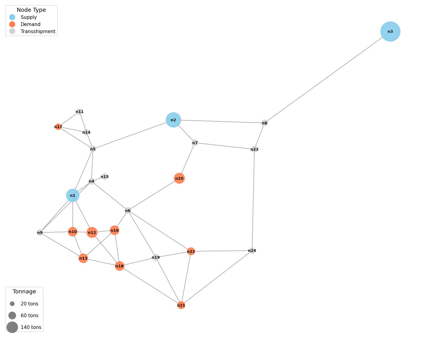
The distribution network comprises 24 nodes: 3 supply nodes, 9 demand nodes, and 12 transshipment nodes. Each of the 42 undirected road segments was modeled as two directed arcs (one in each direction), yielding 84 directed arcs, since vehicles may traverse any road in either direction. The network exhibits a hub-and-spoke topology: the three supply nodes (n1, n2, n3) are centrally positioned with high connectivity, while several demand nodes sit at the network periphery, reachable only through chains of transshipment nodes. This topology has implications for analysis, as peripheral demand nodes are more expensive to serve and more sensitive to vehicle availability at intermediate points. The spatial structure of the network is displayed in Figure 1.

Mathematical Formulation

Objective Function

The model maximizes total demand delivered with a small cost-minimization tie-breaker:

   

where = is a dimensionless cost penalty that breaks ties in favor of lower-cost solutions when multiple distribution plans deliver the same tonnage. Unlike a cost-minimization formulation (which requires all demand to be met as a hard constraint and returns infeasible when it cannot), this demand-maximization approach guarantees a feasible solution for every parameter combination. This property is essential for the Monte Carlo, fleet, and degradation experiments, where many scenarios are evaluated automatically and infeasibility would preclude meaningful statistical comparison.

Sets

Symbol	Description	Size
I	Set of all nodes in the network	||I|| = 24
IS ⊆ I	Supply nodes	||IS|| = 3
ID ⊆ I	Demand nodes	||ID|| = 9
IT ⊆ I	Transshipment nodes	||IT|| = 12
A	Set of directed arcs	||A|| = 84
V	Set of vehicle types	||V|| = 3

Parameters

Symbol	Description	Units
si	Available supply at node i ∈ IS	tons
dj	Required demand at node j ∈ ID	tons
distij	Distance of arc (i, j) ∈ A	meters
capv	Capacity of vehicle type v (1, 2, or 3)	tons
cfv	Fixed cost per meter for vehicle type v	USD/m
cvv	Variable cost per meter-ton for vehicle type v	USD/(m·t)
availiv	Number of vehicles of type v available at node i	integer
B	Total budget	USD
ε	Cost tie-breaking penalty (10-6)	dimensionless

Decision Variables

Symbol	Description	Domain
xijv	Total tons shipped on arc (i, j) using vehicle type v	xijv ≥ 0 (continuous)
yijv	Number of vehicle trips on arc (i, j) using vehicle type v	yijv ∈ ℤ≥0 (integer)
wj	Tons of demand actually delivered to demand node j	0 ≤ wj ≤ dj (continuous)

Constraints

Supply constraint. Net outflow from each supply node cannot exceed available supply:

   

Demand delivery. Net inflow to each demand node must equal or exceed its delivered amount:

   

Demand upper bound. Delivered quantity cannot exceed required demand:

   

Vehicle capacity. Flow on each arc cannot exceed the carrying capacity of assigned trips:

   

Vehicle availability. Total outbound trips from each node cannot exceed vehicle stock:

   

Flow conservation. At transshipment nodes, all inflow must equal all outflow:

   

Budget constraint. Total transportation cost cannot exceed the budget:

   

Because w_j is bounded above by d_j and the objective maximizes ∑w_j, the model delivers as much as possible given the supply, vehicle, and budget constraints. When all demand can be met, the cost tie-breaker selects the cheapest feasible plan.

Solver Implementation

The model was implemented in Python using the PuLP modeling library (version 2.9) and solved with the COIN-OR Branch and Cut (CBC) solver. 

Baseline Model and Budget Selection

The baseline model was solved with a budget of $100,000. This value was chosen because preliminary experimentation revealed that the minimum cost to deliver 100% of demand under the original vehicle fleet is approximately $103,600. Setting the budget just below this threshold ensures that the budget constraint is binding at baseline, producing more informative sensitivity and Monte Carlo results than an overly generous budget. Under an unconstrained budget, all experiments would trivially achieve 100% delivery, eliminating meaningful variation.

Mass balance was verified by confirming that total supply consumed equals total demand delivered (net of transshipment flows) to within numerical tolerance (< 0.01 tons).

Parametric Sensitivity Analysis

To characterize how the system responds to changes in demand, the model was solved repeatedly with total demand scaled by multiplicative factors ranging from 0.80 to 1.25 in increments of 0.05. At each level, every demand node’s requirement was multiplied by the same factor, preserving the relative spatial distribution of demand while varying its magnitude. The budget was held fixed at $100,000 throughout, isolating the effect of demand level on delivery performance.

This design identifies the capacity ceiling  and characterizes the rate of degradation beyond it. Because the model maximizes demand delivered, every scenario produces a feasible solution with a measurable delivery outcome, enabling continuous tracking of delivery performance across the full range of demand levels.

Monte Carlo Simulation

To quantify the robustness of delivery outcomes under joint uncertainty in both demand and transportation costs, a Monte Carlo simulation was conducted in which both parameters were independently perturbed across replications. For each of 200 independent replications:

• Demand perturbation. The demand at each node j was drawn from a normal distribution: , where is the baseline demand and 0.15 is the coefficient of variation (CV). Draws were truncated below at 1.0 ton to prevent non-positive demand.
• Cost perturbation. Both the fixed cost () and variable cost () for each vehicle type v were independently drawn from normal distributions with the same 15% and , where and are the baseline costs. Draws were truncated below at 50% of the baseline value to prevent unrealistically low or negative costs.

The budget remained fixed at $100,000, and the original Ferrer et al. vehicle fleet was used. A fixed random seed (42) ensured reproducibility. This design produced 200 distinct scenarios reflecting realistic joint uncertainty in both demand and cost parameters while preserving the overall scale of the problem.

The demand-maximization framework guaranteed a feasible solution for every replication, enabling construction of full empirical distributions of both delivery and cost outcomes. Ninety-five percent empirical confidence intervals were computed from the 2.5th and 97.5th percentiles of the simulated distributions. The probability of achieving full demand satisfaction ( 99.9%) was estimated as the proportion of replications meeting this threshold.

Fleet Composition Experiment

The fleet composition experiment evaluated the effect of vehicle type on the quantity of aid delivered and the cost of delivery when total fleet carrying capacity was held constant at the level of total demand (250 tons).

Experimental Design

1. Controlled variable: Total carrying capacity. Each fleet configuration provided approximately 250 ton-trips of total capacity, matching the network’s total demand. This ensured that capacity was scarce, forcing the optimizer to make meaningful allocation trade-offs.
2. Fleet configurations. Four configurations were compared:

• All vt1 (small, 1 t): 250 vehicles × 1 t = 250 t
• All vt2 (medium, 2 t): 125 vehicles × 2 t = 250 t
• All vt3 (large, 3 t): 84 vehicles × 3 t = 252 t
• Mixed fleet: 84 vt1 + 42 vt2 + 28 vt3 252 t

3. Randomized vehicle placement. In each replication, vehicles were assigned uniformly at random to one of the three supply nodes (n1, n2, n3). Placement was restricted to supply nodes because goods originate at these locations; vehicles stationed at transshipment or demand nodes would have no cargo to carry on their first dispatch, introducing a confound unrelated to vehicle type. This design isolated the effect of vehicle size on delivery and cost.
4. Network. All 84 directed arcs were available in every replication.
5. Replications and statistical testing. Two hundred independent replications per scenario were conducted (800 optimizations total), each with a fresh random vehicle placement. A fixed random seed (42) ensured reproducibility. Welch’s two-sample t-tests were used for pairwise comparisons of mean demand delivered between the mixed fleet and each single-type fleet, with significance assessed at the =0.05 level.

Note on Comparability with the Baseline Model

The fleet composition experiment is not directly comparable to the baseline model in terms of absolute delivery tonnage. Two key differences account for the gap between the baseline’s 246 tons and the fleet experiment’s approximately 220 tons: (1) the baseline uses the original Ferrer et al. vehicle fleet stationed at six nodes across the network, which provides shorter routing paths to peripheral demand nodes, and (2) with all vehicles originating at supply nodes in the fleet experiment, average per-ton transportation costs are higher, reducing total delivery under the same budget. These differences are intentional: the fleet experiment is designed as a controlled comparison across vehicle types, not as a comparison against the baseline.

Network Degradation Experiment

The network degradation experiment evaluated the effect of asymmetric road damage on relative fleet performance, motivated by the well-documented observation that small vehicles can navigate damaged infrastructure (e.g., rubble-narrowed streets, partially collapsed bridges, and flooded fords) that large trucks cannot.

Equal-Capacity Design

To isolate the routing-flexibility advantage of small vehicles from the confounding effect of total fleet capacity, this experiment used an equal-capacity design. The original Ferrer et al. fleet has unequal total capacity: vt1 = 135 vehicles × 1 t = 135 t, while vt3 = 70 vehicles × 3 t = 210 t. If the original fleet were used, vt3 would start with a 56% capacity advantage that the routing flexibility of vt1 must first overcome. Instead, the vt1 fleet was scaled upward so that both fleets had 210 tons of total capacity: 210 vt1 vehicles × 1 t and 70 vt3 vehicles × 3 t. The scaled vt1 vehicles were distributed across the same nodes as the original fleet, with counts multiplied proportionally (scale factor 1.56). This ensured that any delivery difference between fleets was attributable solely to routing flexibility rather than a capacity asymmetry.

Asymmetric Degradation Model

The experiment modeled differential road accessibility as follows:

1. Road damage states. At each degradation level, a fraction of the 42 undirected road segments were affected. Each affected road was randomly assigned one of two damage states:

• Degraded (probability 0.5): The road was damaged but still passable by small vehicles (vt1). Large trucks (vt3) could not navigate the obstruction.
• Destroyed (probability 0.5): The road was impassable for all vehicle types.

2. Asymmetric arc sets. For each replication, the optimization model was solved separately for each fleet using fleet-specific arc sets:

• All vt1 fleet: surviving arcs = intact + degraded roads (small vehicles can navigate damaged infrastructure)
• All vt3 fleet: surviving arcs = intact roads only (large trucks are blocked by damaged roads)

3. Vehicle placement. Vehicles were stationed at the same nodes as the original Ferrer et al. dataset, with vt1 counts scaled proportionally to equalize total fleet capacity.
4. Degradation levels. Six levels were tested: 0%, 10%, 20%, 30%, 40%, and 50% of road segments affected.
5. Replications. Fifty replications per cell (600 total optimizations). Budget was fixed at $100,000 with baseline demand. A fixed random seed (42) ensured reproducibility.

Statistical testing. Welch’s t-tests compared vt1 versus vt3 delivery at each degradation level, with significance assessed at =0.05. Bootstrap confidence intervals (2,000 resamples) were computed for the delivery difference (vt1 – vt3) at each degradation level.

Model Validation

The model’s correctness was verified through several checks. First, the CBC solver confirmed that optimality conditions were satisfied for every solve (status = Optimal). Second, mass balance was verified at baseline by confirming that total supply consumed equals total demand delivered to within numerical tolerance (< 0.01 tons), ensuring that aid is neither created nor destroyed in transit. Third, programmatic assertions confirmed that the model function implements demand-maximization (LpMaximize), includes demand-met decision variables (w_j), and applies the cost tie-breaking penalty (). Fourth, the demand-maximization framework guaranteed that every scenario produced a feasible, measurable result.

Software and Reproducibility

All analyses were conducted in Python 3.13 using the following packages: PuLP (linear programming modeling and CBC solver interface), NumPy and pandas (data manipulation), SciPy (statistical testing), NetworkX (network construction and layout), Matplotlib (visualization), and tqdm (progress monitoring). The complete analysis code is provided as a Jupyter notebook to ensure full reproducibility.

Results

Descriptive Statistics

The distribution network comprises 24 nodes connected by 84 directed arcs (42 undirected road segments modeled bidirectionally). Of the 24 nodes, 3 are supply depots, 9 are demand points, and 12 are transshipment nodes. Total available supply is 280 tons, distributed across the three supply nodes, while total required demand is 250 tons across the nine demand nodes, yielding a supply-to-demand ratio of 1.12. Arc distances range from approximately 3,000 m to over 80,000 m (mean 30,000 m). The vehicle fleet comprises three types: vt1 (1 t capacity, 100 km/h), vt2 (2 t capacity, 80 km/h), and vt3 (3 t capacity, 60 km/h), each with distinct fixed costs per meter ($0.02, $0.04, and $0.05, respectively) and a common variable cost of $0.001/(m·t). 

Baseline Model Results

Under a $100,000 budget with the original Ferrer et al. vehicle fleet, the model delivered 246 tons out of 250 tons of total demand (98.4%). The total transportation cost was $99,815, which consumed 99.8% of the available budget at a unit cost of $405.75 per ton delivered. Mass balance was verified: supply consumed equaled demand delivered to within numerical tolerance (< 0.01 tons). The 4-ton shortfall (1.6% of demand) represents the marginal demand that cannot be served within the remaining $185 of budget headroom. The baseline solution utilized 30 active routes and required approximately 328 vehicle trips. This near-complete but not-quite-full delivery demonstrates that the system operates at the margin of its budget constraint, where small changes in demand or cost parameters produce measurable shifts in delivery outcomes.

Parametric Sensitivity Analysis

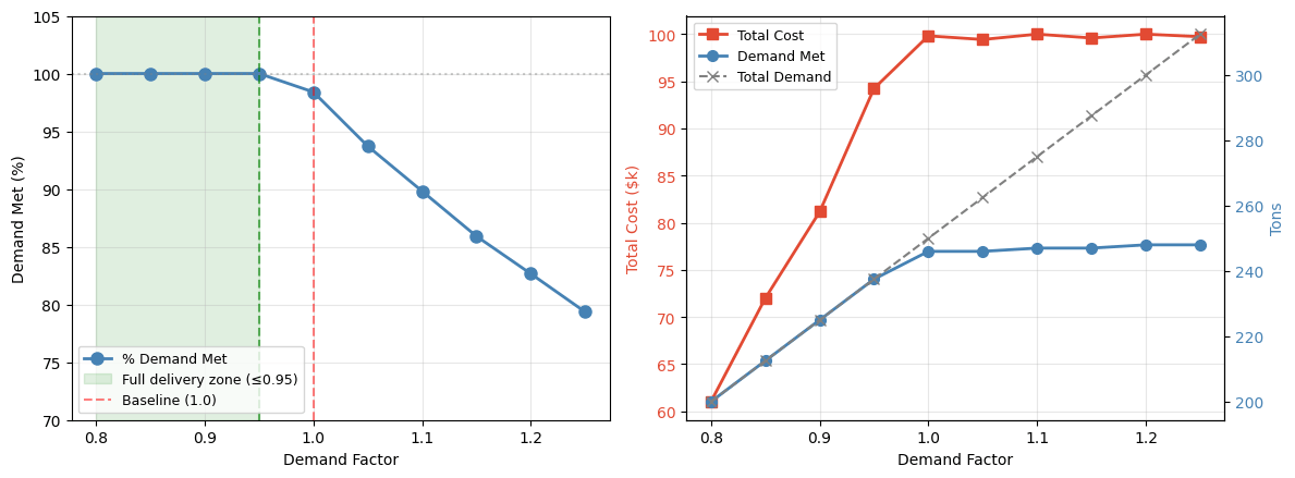
The results of the parametric sensitivity analysis are presented in Table 1 and Figure 2. The model achieved 100% demand satisfaction for all demand factors from 0.80 through 0.95 (200–237.5 tons). At the baseline factor of 1.00, delivery dropped to 98.4% as the budget constraint became binding. Beyond this point, delivery saturated near 246–248 tons as the budget ceiling prevented the model from activating additional routes: at factor 1.25 (312.5 tons), only 79.4% of demand was met.

Demand Factor	Total Demand (t)	Demand Met (t)	% Met	Cost (USD)
0.80	200.0	200.0	100.0%	$61,032
0.85	212.5	212.5	100.0%	$71,907
0.90	225.0	225.0	100.0%	$81,166
0.95	237.5	237.5	100.0%	$93,143
1.00	250.0	246.0	98.4%	$99,815
1.05	262.5	246.0	93.7%	$99,416
1.10	275.0	247.0	89.8%	$99,965
1.15	287.5	247.0	85.9%	$99,572
1.20	300.0	248.0	82.7%	$99,994
1.25	312.5	248.0	79.4%	$99,728

The capacity ceiling was identified at demand factor 0.95 (237.5 tons): below this level, 100% delivery was achieved; above it, delivery degraded monotonically as additional demand exceeded the budget’s capacity to fund additional routing. Transportation cost increased with demand in the full-delivery zone but plateaued near $100,000 once the budget was fully consumed. The gap between total demand and demand delivered widened steadily above the ceiling, indicating that each additional ton of demand above 237.5 tons was progressively harder to serve within the fixed budget.

Within the full-delivery range (factors 0.80–0.95), cost sensitivity was approximately 1.75% cost change per 1% demand change, indicating a super-linear relationship between demand and transportation cost.

Monte Carlo Simulation

Across 200 replications with independently perturbed demand (CV = 15%) and cost parameters (CV = 15% on both fixed and variable costs per vehicle type), the model delivered a mean of 242.8 tons (SD = 10.0 tons), satisfying an average of 97.2% of demand. The 95% empirical confidence interval for demand delivered was [224.6, 261.8] tons. Full demand satisfaction ( 99.9%) was achieved in 69 of 200 replications (34.5%), confirming that under the $100,000 budget with joint demand and cost uncertainty, full delivery is possible but not assured. The budget constraint was binding in 60 of 200 replications (30%), indicating that the $100 ceiling frequently limited additional deliveries even when feasible demand remained. 

Metric	Mean	SD	Min	Max	95% CI
Demand met (tons)	242.8	10.0	218.0	270.2	[224.6, 261.8]
Demand met (%)	97.2%	3.5%	83.7%	100%	—
Total cost (USD)	$94,851	$7,898	—	—	[$72,610, $100,000]
Cost CV	8.3%	—	—	—	—

The cost coefficient of variation was 8.3%, indicating moderate cost variability across joint demand and cost scenarios. The upper bound of the cost confidence interval was capped at $100,000, confirming that the budget was frequently binding. The demand satisfaction distribution was left-skewed, with most replications clustered near 95–100% delivery and a tail extending to approximately 84%, corresponding to scenarios where both demand spiked and costs were drawn high simultaneously.

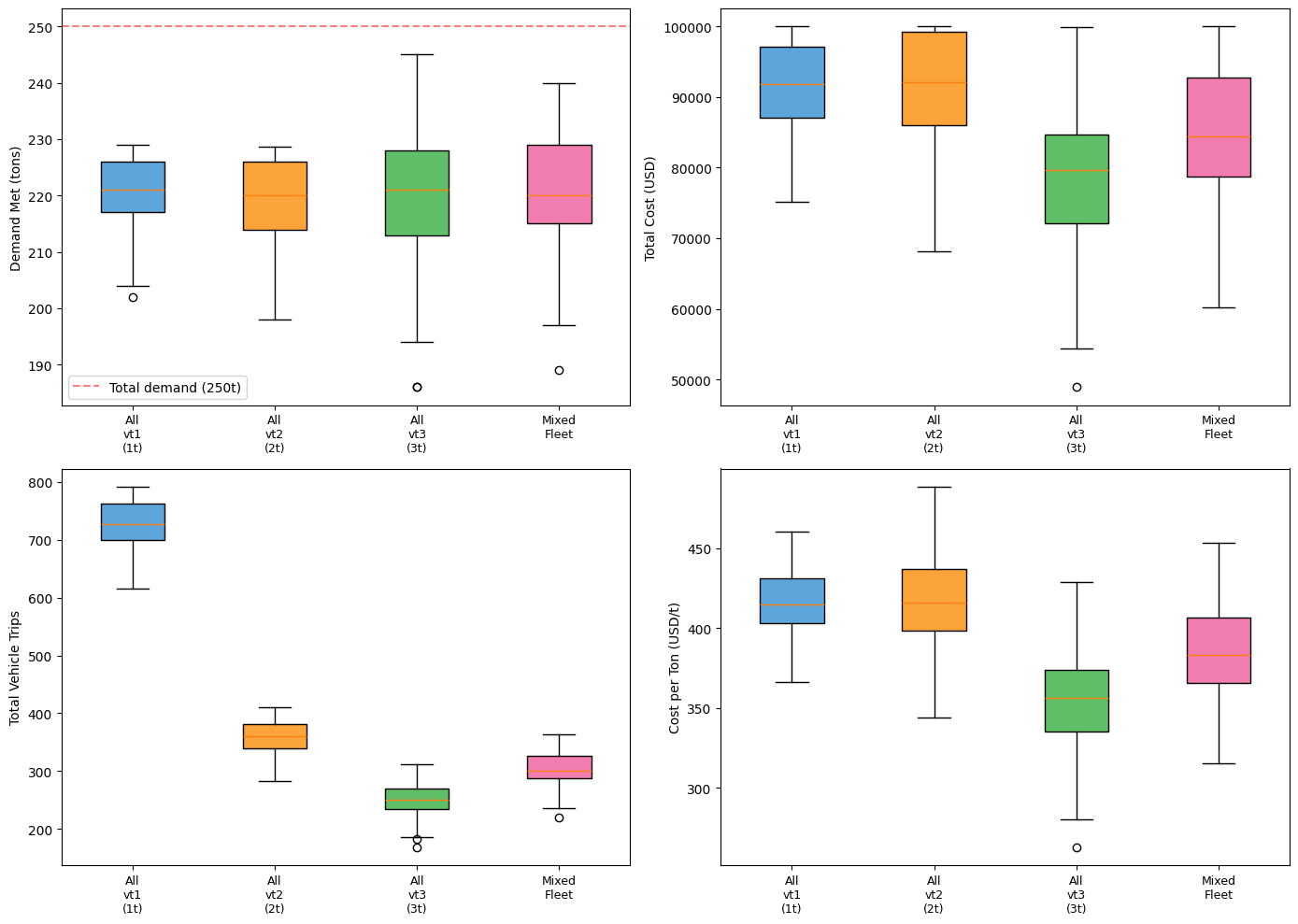
Fleet Composition Experiment

Delivery Performance

Across 200 replications per fleet configuration, all four configurations delivered approximately 88% of total demand (219–221 tons out of 250 tons). The 12% shortfall relative to total demand reflects the higher per-ton routing costs when all vehicles originate at supply nodes rather than being distributed across intermediate network positions. No single fleet type achieved full delivery.

Fleet Configuration	Mean (t)	SD (t)	Min (t)	Max (t)	Mean % Met
All vt1 (1 t)	220.6	6.0	202.0	229.0	88.2%
All vt2 (2 t)	219.0	7.4	198.0	228.6	87.6%
All vt3 (3 t)	219.9	10.9	186.0	245.0	88.0%
Mixed fleet	221.0	9.4	189.0	240.0	88.4%

Mean demand delivered was remarkably similar across fleets (range: 2.0 tons). Pairwise Welch’s t-tests comparing the mixed fleet to each single-type fleet yielded only one statistically significant difference: Mixed vs. All vt2 ( = +2.0 t, t = 2.33, p = 0.020). Comparisons against vt1 and vt3 were not statistically significant (p>0.28). These results indicate that, for this network and demand structure on an intact road network, fleet composition has a limited effect on the total quantity of aid delivered.

Comparison	Δ (tons)	t-statistic	p-value	Significance
Mixed vs. All vt1	+0.4	0.54	0.592	ns
Mixed vs. All vt2	+2.0	2.33	0.020	*
Mixed vs. All vt3	+1.1	1.08	0.281	ns

Note: Significance levels: * p < 0.05; ns = not significant.

Cost Efficiency

While delivery volumes were similar, cost structures differed substantially across fleet configurations.

Fleet Configuration	Mean Cost (USD)	Mean $/ton	Mean Trips	Mean Active Routes
All vt1 (1 t)	$91,731	$415	727	16.5
All vt2 (2 t)	$91,283	$416	360	16.4
All vt3 (3 t)	$78,444	$356	250	17.0
Mixed fleet	$85,530	$386	306	28.6

The all-vt3 (large vehicle) fleet operated at a mean cost of $78,444 (approximately $356 per ton delivered) compared to approximately $415–$416 per ton for both the vt1 and vt2 fleets. The mixed fleet fell in between at approximately $386 per ton. This approximately 15% cost advantage of large vehicles arises because they amortize fixed per-trip costs over more tonnage per trip, requiring only 250 trips on average compared to 727 for the all-vt1 fleet.

Delivery Variance

The all-vt3 fleet exhibited the highest standard deviation in delivery (10.9 t vs. 6.0 t for vt1). With only 84 vehicles distributed across three supply nodes, random placement produced more uneven allocations (e.g., one supply node may receive disproportionately many vehicles while another receives too few), making delivery outcomes less predictable. The all-vt1 fleet, with 250 vehicles, produced more uniform coverage and therefore more consistent delivery.

Routing Flexibility

The mixed fleet activated the most routes on average (28.6 active arcs per replication vs. 16.4–17.0 for single-type fleets), suggesting that fleet diversity enables the optimizer to exploit a broader set of routing options. This routing flexibility likely explains the mixed fleet’s slight delivery advantage over vt2, as the optimizer can simultaneously use small vehicles for short peripheral routes and large vehicles for high-volume trunk routes.

Network Degradation Experiment

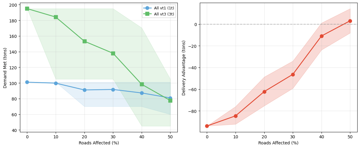
Fleet Resilience Under Asymmetric Road Damage

Using equal-capacity fleets (210 t each) at the original Ferrer et al. node positions, the experiment revealed a stark contrast in how small and large vehicles respond to increasing infrastructure damage. At 0% degradation, the vt3 fleet delivered 195.0 tons compared to 101.0 tons for the vt1 fleet — a 94-ton gap driven entirely by the cost-efficiency advantage of large vehicles, which carry more payload per trip and therefore consume less budget per ton delivered. As degradation increased, this gap narrowed progressively due to the asymmetric loss of road access.

Roads Affected	vt1 Mean (t)	vt3 Mean (t)	Δ (vt1 − vt3)	t-statistic	p-value	Significance
0%	101.0	195.0	-94.0	—	< 0.001	***
10%	96.7	170.8	-74.2	-12.18	< 0.001	***
20%	96.0	159.4	-63.4	-9.40	< 0.001	***
30%	89.3	122.5	-33.2	-4.66	< 0.001	***
40%	87.7	92.0	-4.3	-0.58	0.565	ns
50%	79.5	67.8	+11.7	2.26	0.027	*

Note: Significance levels: *** p < 0.001; * p < 0.05; ns = not significant.

Crossover Point

At 50% degradation, the vt1 fleet significantly outdelivered vt3 by 11.7 tons (79.5 t vs. 67.8 t, p=0.027) — a statistically significant crossover. At 40% degradation, the gap had nearly closed (=-4.3 t, p=0.565, not significant), indicating the crossover threshold lies between 40% and 50% of roads affected.

Differential Degradation Rates

From 0% to 50% degradation, vt3 delivery dropped from 195.0 t to 67.8 t (a 65% decline), while vt1 dropped from 101.0 t to 79.5 t (a 21% decline). This stark asymmetry confirms that large vehicles are highly sensitive to network damage because they lose access to both degraded and destroyed roads, while small vehicles lose access only to destroyed roads.

Arc Availability

Roads Affected	vt1 Arcs	vt3 Arcs	Arc Advantage (vt1 − vt3)
0%	84.0	84.0	0.0
10%	79.9	76.0	+3.9
20%	75.5	68.0	+7.5
30%	71.5	58.0	+13.5
40%	67.6	50.0	+17.6
50%	63.2	42.0	+21.2

At 50% degradation, vt1 retained access to a mean of 63.2 directed arcs while vt3 retained only 42.0 — a 21-arc advantage. This growing gap in usable network is the mechanism driving the crossover: as degradation increases, the vt1 fleet’s access to degraded roads increasingly compensates for its lower cost efficiency per trip.

Cost Efficiency Under Degradation

At 0% degradation, the cost per ton was $331 for vt1 and $411 for vt3. At 50% degradation, these values shifted to $202 for vt1 and $98 for vt3. The vt3 fleet’s low cost per ton at high degradation is misleading: while each ton delivered by vt3 is inexpensive, the fleet delivers far fewer tons overall because it cannot access much of the network. The vt1 fleet, by contrast, continues to reach demand nodes through degraded roads, achieving higher total delivery at moderate cost per ton.

Discussion

Across all four experiments, budget emerged as the primary binding constraint on delivery performance. This finding remained true in all conditions–stable or unstable–and fleet compositions. Under a $100,000 budget with the original vehicle fleet, the model delivered 246 out of 250 tons (98.4%) of demand while using $99,815, which is 99.8% of the available budget. This shows that the system is almost completely limited by cost. The near-complete delivery and minimal remaining budget capacity indicate that even small increases in demand or transportation costs can lead to measurable reductions in delivery performance. This finding is consistent with prior work by Kandil (2025), who noted that cost constraints inhibit the reach and efficiency of disaster response in post-disaster distribution planning¹⁰.

Additionally, the parametric sensitivity analysis supports this constraint by showing a clear capacity ceiling at demand factor 0.95 (237.5 tons). When demand is at or below the demand factor of 0.95, the system could meet 100% of demand. However, above a demand factor of 0.95, the delivery stops increasing and saturates around 246-248 tons. This occurs because the budget constraint prevents the system from delivering more, since more nodes and routes need to be activated. The system physically cannot deliver more without increasing the budget. The results also show that costs increase faster than demand, with a 1.75% increase in costs per 1% increase in demand, indicating super-linear cost scaling as delivering to harder-to-reach locations becomes increasingly expensive, quickly draining the budget.

The Monte Carlo simulation shows what happens under more realistic conditions, with variable demand and costs. In this experiment, the model was run 200 times with 15% variation in both demand and cost parameters. On average, the system delivered 97.2% of demand, but only 34.5% of the simulations fully met demand, meaning that in most cases, some aid was left undelivered. The system usually performs well, but it is not reliable under changing conditions as it is sensitive to uncertainty. Additionally, the delivery amounts had a standard deviation of 10.0 tons, meaning small changes can drastically impact how much aid is delivered. Even though the cost variability was moderate, with a coefficient of variation of 8.3%, the system frequently hit the $100,000 budget limit. Thus, this experiment emphasizes that the budget is the main constraint, even when conditions are changing.

The fleet composition experiment results show that the vehicle type mainly affects efficiency rather than total delivery. When capacity equaled total demand and vehicles were placed at supply nodes, all four fleet configurations delivered approximately 88% of demand. However, cost efficiency was the primary differentiator: large vehicles (vt3) delivered at $365 per ton, compared to 416 per ton for small (vt1) and medium (vt2) vehicles. The mixed fleet performed better overall, achieving the highest mean delivery of 88.4% and using more active routes (28.6 active routes compared to 16-17 for single-type fleets). These results suggest that utilising a variety of vehicle types allows the system to use more routes and have greater routing flexibility. This is consistent with the findings of Eberhardt et al. (2025) who found that combining vehicle types rather than a single homogeneous fleet results in better route allocation and utilization¹¹.

Additionally, the network degradation experiment to test fleet resilience shows how road damage influences the effectiveness of vehicle fleets. At 0% degradation, larger vehicles perform much better, with vt3 delivering 195 tons compared to 101 tons for vt1, mainly because they are more cost-efficient. However, as roads become unviable, large vehicles (vt3) lose effectiveness quickly, decreasing by about 26 tons for every 10% increase in road damage. On the other hand, small vehicles (vt1) only decrease by about 4 tons per 10%, showing that they are much more stable in road failures. At 40% degradation, the gap between large vehicles and small vehicles was statistically indistinguishable; yet at 50% road degradation, small vehicles (vt1) outdeliver large trucks (vt3) by 11.7 tons (p = 0.027). This finding demonstrates that small vehicles are significantly more effective under network degradation and better able to handle damaged infrastructure. These results align with the broader observation in the humanitarian logistics literature that post-disaster road networks are rarely fully intact, and that logistical plans must account for partial and asymmetric road availability (e.g. Holguín-Veras et al)¹².

These findings highlight the value of optimization models in humanitarian logistics, particularly for improving resource allocation and distribution efficiency. While many existing studies assume stable transportation networks, this study explicitly incorporates infrastructure disruption and demonstrates how it affects delivery outcomes. The results show that network damage significantly changes which vehicle types are most effective, which supports the idea that real-world disaster conditions must be considered in logistical planning. In addition, this study extends previous work by examining the interaction between budget constraints, uncertainty, and fleet composition within a single framework. By doing so, it addresses a gap in the literature and provides a more realistic representation of post-disaster logistics systems.

The findings in this study suggest a real-world strategy for policy implications. Under budget-constrained operations on intact infrastructure, large vehicles should be used as they maximize both delivery volume and cost efficiency. Under severe infrastructure damage ( 50% of roads affected), small vehicles should be used as they become more effective and outperform large trucks in absolute delivery because they can still reach blocked or narrow routes. This supports a two-phase strategy: first, deploying small vehicles for initial penetration into heavily damaged areas where road access is critical immediately after a disaster. Then, larger vehicles are used as roads are cleared, and cost efficiency becomes the binding constraint. This two-phase strategy, using the results of the study, optimizes throughput and network reach in disaster response.

Conclusion

This study developed a mixed-integer linear programming (MILP) model to analyze post-disaster last-mile distribution using data from the 2010 Haiti earthquake. This model was used to run a series of computational experiments examining how budget constraints, demand variability, fleet composition, and infrastructure damage jointly affect the effectiveness of aid delivery. 

One of the key findings is that budget is the primary limiting factor in aid delivery. The model could not fully meet demand, even when total supply exceeded demand, as it quickly used up the $100,000 budget. The capacity ceiling of the system was identified. The model also shows that uncertainty in demand and cost reduces the strategy’s reliability, and that the effectiveness of different vehicle types was significantly dependent on infrastructure conditions. 

Overall, these results highlight that, contrary to resource availability, the combined constraints of cost, damaged infrastructure, and uncertainty in conditions are the key issue in humanitarian logistics efforts. This demonstrates that humanitarian logistics teams should focus on designing logistics systems that can adapt to variable and degraded conditions, instead of simply stockpiling aid.

That said, this study has several limitations. The model does not account for changes in the transportation network, time-dependent decisions, or coordination between multiple organizations. As a result, the model should be interpreted as a simplified representation of real disaster logistics systems. Future studies could apply the model to other disaster scenarios or more recent datasets to improve its generalizability and incorporate these variables into time-based decision processes. For instance, future research might extend this framework by incorporating stochastic demand into the facility location stage and testing the two-phase fleet deployment strategy under dynamic road-clearing conditions.

Ultimately, although simplified, this model provides a foundational decision-support framework that zooms in on last-mile distribution, and it demonstrates that optimization-based distribution can play a crucial role in improving humanitarian logistics for earthquake-prone areas. Most notably, based on the key finding that small vehicles outperform large trucks once road degradation exceeds 50%, it is suggested that humanitarian organizations prioritize fleet flexibility over carrying capacity in the immediate aftermath of a disaster. By building on this work with more comprehensive data and complex variables, future research can help humanitarian organizations to deliver life-saving aid in disasters.

Acknowledgements

I would like to thank Dr. Jonathan Holt of Duke University for his guidance and support on this research.

References

1. S. M. Harle, S. Sagane, N. Zanjad, P.K.S. Bhadauria, H.P. Nistane. Advancing seismic resilience: Focus on building design techniques. Structures. Vol. 66, pg. 106432, 2024, https://doi.org/10.1016/j.istruc.2024.106432. [↩]
2. F. Fiedrich, F. Gehbauer, U. Rickers. Optimized resource allocation for emergency response after earthquake disasters. Safety Science. Volume 35, Issues 1-3, pg. 41-57, 2000, https://doi.org/10.1016/S0925-7535(00)00021-7. [↩]
3. M.C. Hoyos, R.S. Morales, R. Akhavan-Tabatabaei. Or models with stochastic components in disaster operations management: A literature survey. Computers & Industrial Engineering, Vol. 82, pg. 183-197, 2015, https://doi.org/10.1016/j.cie.2014.11.025. [↩] [↩] [↩]
4. Khater, M. Humanitarian assistance in cases of natural disasters and the 2023 earthquake in Turkey and Syria. Environment Conservation Journal, 24(2), pg. 423-433, 2023, https://doi.org/10.36953/ECJ.22842584. [↩] [↩]
5. R. Margesson, M. Taft-Morales. Haiti earthquake: Crisis and response. Library of Congress Washington D.C. Congressional Research Service, 2010, https://apps.dtic.mil/sti/html/tr/ADA516429/. [↩] [↩]
6. United Nations Development Programme. Haiti technical guide for debris management. United Nations Development Programme, 2017, https://www.undp.org/publications/haiti-technical-guide-debris-management. [↩]
7. A. Ilabaca, G. Paredes-Belmar, P.P. Alvarez. Optimization of Humanitarian Aid Distribution in Case of an Earthquake and Tsunami in the City of Iquique, Chile. Sustainability, 12(2), pg. 819, 2022, https://doi.org/10.3390/su14020819. [↩] [↩]
8. J.M. Ferrer, F.J. Martín-Campo, M.T. Ortuño, A.J. Pedraza-Martínez, G. Tirado, B. Vitoriano. Multi-criteria optimization for last mile distribution of disaster relief aid: Test cases and applications. European Journal of Operational Research, Vol. 269, pg. 501-515, 2018, https://doi.org/10.1016/j.ejor.2018.02.043. [↩] [↩] [↩]
9. L. Cheng, A.J. Hertelendy, A. Hart, L.S. Law, R. Hata, G. Nouaime, F. Issa, L. Echeverri, A. Voskanyan, G.R. Ciottone. Factors associated with international humanitarian aid appeal for disasters from 1995 to 2015: A retrospective database study. PLoS One, 18(6), e.0286472, 2023, 10.1371/journal.pone.0286472. [↩]
10. A. Kandil. Towards a Sustainable Cost Optimization Model for Humanitarian Supply Chains in Disaster Response. Social Science Research Network Electronic Journal, 2025, https://doi.org/10.2139/ssrn.5747682. [↩]
11. K. Eberhardt, F. Diehlmann, M. Lüttenberg, F.K. Kaiser, F. Schultmann. A combined fleet size and mix vehicle routing model for last-mile distribution in disaster relief. Progress in Disaster Science, Vol. 26, 100411, 2025, https://doi.org/10.1016/j.pdisas.2025.100411. [↩]
12. J. Holguín-Veras, M. Jaller, Luk. Wassenhove, N. Pérez, T. Wachtendorf. On the unique features of post-disaster humanitarian logistics. Journal of Operations Management, Vol. 30, pg. 492-506, 2012, https://doi.org/10.1016/j.jom.2012.08.003. [↩]