Using Neural Networks to Predict the Likelihood of Floods

Abstract

Floods are a growing threat to human life, infrastructure, and economies around the world. They are driven by factors such as extreme rainfall, humidity, and land use patterns. Traditional hydrologic models (e.g., Soil & Water Assessment Tool (SWAT), Hydrologic Modeling System (HEC-HMS)) often struggle to deliver accurate, re99al-time predictions when presented with rapidly changing situations. This study developed a machine-learning-based flood- prediction system using the Bangladesh Flood Prediction Dataset, which spans diverse climatic and geographic areas within the country. After cleaning and standardizing ten key environmental factors (e.g., rainfall, humidity, temperature, pressure, etc.), exploratory data analysis was conducted using the Pearson correlation heatmapping to identify the strongest predictors of flood incidents. Two feed-forward neural networks were then tuned and trained with varying layer counts and neuron counts, and compared to logistic regression, multiple linear regression, and random- forest classifier. The best-performing neural-network architecture (six hidden layers of 60 Rectified Linear Unit (ReLU) neurons) achieved 98.89 % accuracy on the validation data after 100 epochs, followed by logistic regression (98.66 %), Random Forest Classifier (98.55 %), and linear regression (91.78 %). These results therefore indicate that relatively straightforward deep-learning architectures can match or exceed both traditional physics-based forecasts and alternative machine-learning methods. By using a country-wide dataset rather than river-specific measurements, this methodology offers scalable, generalizable flood-risk prediction suitable for data-scarce regions with similar characteristics as Bangladesh. Further future work can explore the integration of land-use and infrastructure predictors, time-series models, and automated hyperparameter optimization to further enhance early-warning capabilities.

Introduction

A flood is an overflow of water onto land normally dry land. Flooding can be caused by numerous factors such as heavy rainfall, deforestation, and dam failures. Floods can last for days or even weeks, as opposed to flash floods which last for short periods of time, and can cause immense loss of human lives and the economy of affected areas¹. This type of natural disaster is influenced by many environmental and human factors such as rainfall intensity, topography and urbanization². Floods are especially important to study because they inflict devastating impacts on the lives of humans, the economy, and the environment. According to the World Meteorological Organization (WMO), between 1994 and 2013 nearly 2.5 billion people were impacted by floods around the world and floods have caused over $40 billion in damage every year. The WMO also reports that the impact of these floods is also rising at a very rapid pace, as the population residing in flood-prone areas has grown by 24% between 2000 and 2015³. The frequency and danger of such floods also indicate the importance of reliable flood forecasts in order to provide the necessary precautions and evacuations.

Conventional flood forecasting models, which rely on sophisticated statistical and hydrologic computations such as the Soil and Water Assessment Tool (SWAT) or Hydrologic Modeling System (HEC-HMS), have played a critical role in flood forecasting.  These hydrologic models represent the watershed and physical processes explicitly. SWAT is a basin-scale model used to simulate the quality and quantity of surface and ground water, and is widely used to predict the environmental impact of land use and climate change⁴. HEC-HMS, on the other hand, is designed to simulate the hydrologic processes of certain watershed systems. It integrates various hydrologic procedures such as hydrologic routing, event infiltration and unit hydrographs, which makes it suitable for a variety of applications such as flood prediction and surface erosion studies. However, these models are considered to be imperfect, when used to forecast dynamic and rapidly-changing conditions. A study by Mosavi et al.⁵ confirms that these models are often rigid, require much adjustment, and are generally not capable of making accurate short-term or real-time predictions. This is due to their reliance on predetermined parameters and assumptions that cannot adapt to unexpected weather or hydrologic changes. Therefore, these flaws have the potential to cause delayed warnings and pose safety risks to human lives.

In contrast to those traditional models, recent technological advancements in machine learning have introduced very flexible models that are capable of learning subtle patterns from large and dynamic data. Machine learning algorithms, such as Neural networks or Long Short-Term Memory networks, excel at short-term predictions by detecting interdependencies within data streams. Recent work has shown that deep learning models can match or exceed the capabilities of traditional hydrologic models in accuracy; large-sample machine learning studies have demonstrated that data-driven models can learn regional and local hydrologic behaviour when trained on large datasets.

More recently, the field has moved towards geospatial artificial intelligence (GeoAI) and hybrid hydrological machine learning models which bridge data-driven analysis and spatial / geospatial information. GeoAI combines geospatial data from satellite imagery or remote sensing, with deep learning models such as convolutional neural networks (CNNs) or transformers to improve flood mapping. Hybrid hydrological machine learning models, on the other hand, use output or physical constraints from process models (such as SWAT / HEC-HMS outputs) to improve generalization to unseen or changing environments and reduce the need for massive datasets.

An example of such a study is one that is conducted by Shi et al.⁶ on flood predictions in South Florida, in which the use of machine learning algorithms is demonstrated in flood risk prediction. This model has several strengths over traditional physics-based models. Most notably, the deep learning models rivaled or outperformed conventional models in terms of error rates while gaining a significant computational boost—reportedly at least 500 times faster than traditional models⁶. Such efficiency enables rapid predictions, which is critical for real-time flood prediction as well as emergency responses. Although the model’s predictions are particularly accurate, its specific focus on Miami River and surrounding areas might confine it to South Florida only. Thus, its strength and applicability to other regions of the world with different environmental factors might be limited, making it not widely applicable. Also, their utilization of a large range of river-specific variables might confine it to areas having a large array of river data, which might render it inapplicable in areas having limited river data.

This study overcomes this limitation by using a dataset – Bangladesh Flood Prediction Dataset⁷ – which collects climatic and hydrologic data from across Bangladesh. This national dataset uses multiple geographical and climatic parameters and therefore possesses a broader model training base. Compared to Shi et al.’s approach, this model considers a wider set of environmental factors such as temperature, rainfall intensity, humidity, and pressure and is consequently able to provide a more detailed estimation of flood probability. This approach also demonstrates the ability to estimate flood probabilities even for sparse data locations; thus it is more applicable in real-life, data-scarce environments.

To achieve this, this paper uses classification neural networks on a diverse dataset in order to build an efficient and scalable model. By doing that, the model can make predictions that are not geographically specific, but applicable to a wider range of environments with similar climatic and monitoring characteristics.

Methodology

To analyze the probability of flooding in different situations, this study uses the Bangladesh Flood Prediction Dataset⁷ from Github. The dataset has a heterogeneous range of features relevant to flood prediction such as geographical, hydrologic parameters spanning from the years 1948 to 2013. It has variables including latitude, rainfall, and wind speed. The wide range of variables gives a broad overview of the environmental variables that influence floods and the complex interplay between environmental flood risk variables. Furthermore, the dataset collects data on a city level, which allows for more in-depth analysis of the country’s regional variation. It provides a binary “Flood” column which represents whether flooding occurred (labeled 1) or not (labeled 0). The author compiled the flood labels from sources such as news reports and national flood reports, and the flood variable reports flood occurrence at a specific station in a given month of a year.

Of the original 20,544 rows in the dataset, 4,493 (21.87%) rows had flood labels while 16,051 (78.13%) were missing flood labels. Thereby, all unlabeled rows were excluded from training so that incorrect assumptions about flood occurrences were not made.

To preprocess the dataset for modeling, several procedures were implemented to clean the dataset. The variables were normalized through standardization to ensure that all variables have an equal contribution to the model’s output. 

To further investigate the dataset, exploratory data analysis was conducted in order to examine the relationship between the variables.

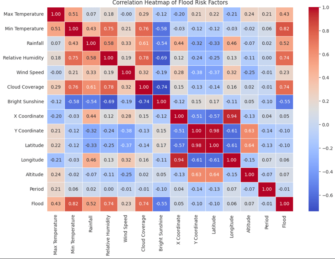
A correlation heatmap (Figure 1) was derived from the Pearson correlation coefficients to examine the correlations among various environmental factors and the flood occurrence. The majority of the variables are revealed to have weak to moderate associations with flood occurrence according to the heatmap. However, some specific factors stand out among them. Notably, Minimum Temperature is strongly correlated with flood occurrence (r = 0.82), followed by cloud coverage and relative humidity (r = 0.74), rainfall (r = 0.52), and maximum temperature (r = 0.43). Bright sunshine, however, negatively correlates with floods (r = -0.55). These results show that none of the variables are entirely predictive on their own, but combinations of those climatic factors can be strong predictors of floods. Feature importances were also computed from a Random Forest Classifier using the model’s impurity-based feature importance. A SHAP summary of the neural network model was also evaluated to validate the feature importance ranking.

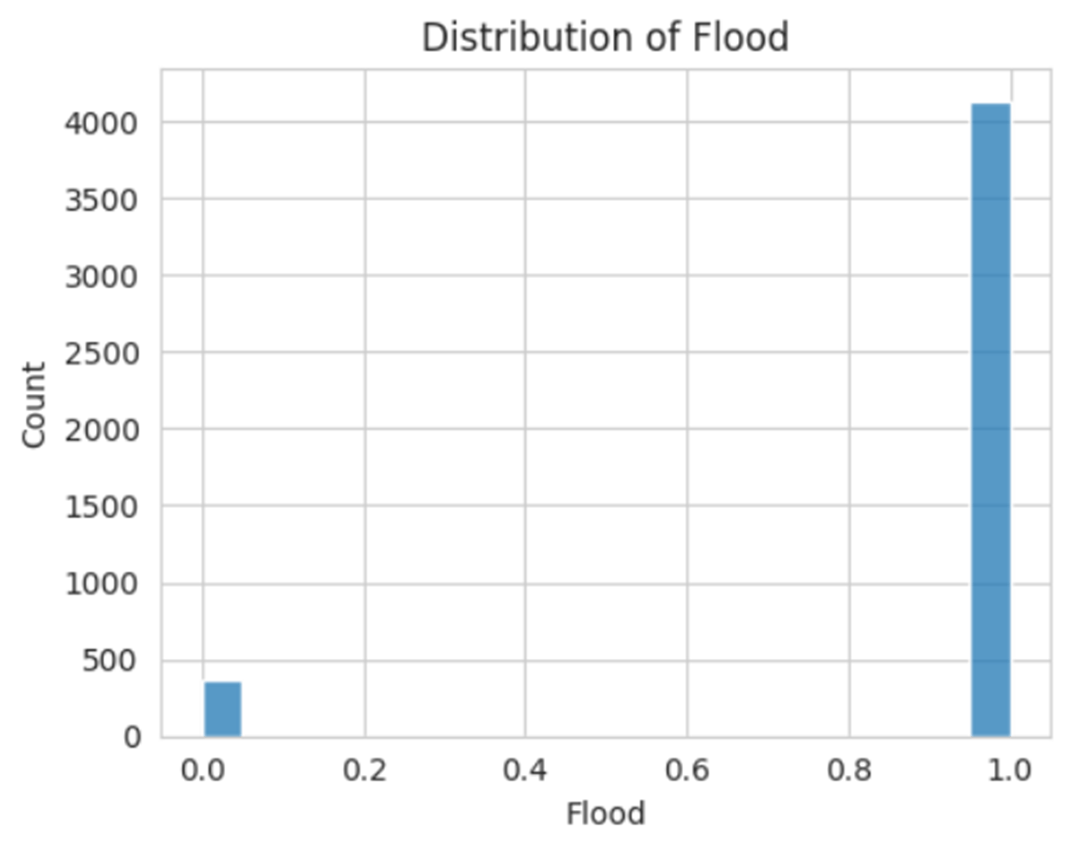
However, there is some notable class imbalance between the number of Flood occurrences and the number of No Flood Occurrences, as shown in Figure 2. Specifically, the dataset contains a total of 4132 Flood occurrences and 361 No Flood occurrences. The imbalance between the number of flood occurrences within the dataset can have an impact on the effectiveness and the bias of the model.

To analyze the diverse flood-causing factors efficiently, a classification neural network was used as the primary algorithmic approach. As the objective of the task is to predict the chances of a flood event, a classification neural network is appropriate. Classification neural networks are well-suited to calculate the probability of a condition belonging to a specific class, which, in this case, is either “flood-prone” or “flood-safe” state. A classification neural network also enables the model to detect the subtle, non-linear connections between the variables, thus making it a perfect tool to predict flood risk. To train the model, a chronological (time-based) holdout was used: the dataset was sorted based on the month and year of the event, and split into training, validation, and test sets in an 7:2:1 ratio, respectively.

The classification neural network model consists of 6 hidden layers with 60 neurons each and uses the Rectified Linear Unit (ReLU) activation function. To determine the most efficient structure, two different tuning methods were evaluated. A grid search was performed by testing out different hyperparameter combinations (layers and neuron count for uniform-layer neural networks models; number of layers and the number of neurons in the first hidden layer for a funnel shaped network where each layer has half the neurons of the previous one), training each architecture for 100 epochs and selecting the best model based on validation accuracy.

In the first approach, the model was constructed with an input layer followed by a number of hidden layers, each having a uniform number of neurons. Layer (4, 6, 8, 10 layers) and neuron (20, 30, 40, 50, 60

neurons) combinations were tested systematically to determine their impact on the performance of the model.

The second approach evaluated architectures in which the number of neurons decreased sequentially in powers of 2 per layer. Starting from a larger number of neurons (256, 128, 64, 32 neurons) and decreasing gradually down to smaller sets of neurons, different configurations were tested by adjusting the starting point and the number of hidden layers.

The architectures of both tuning methods were trained and tested using 100 epochs, and validation accuracy (on a 20% hold-out set) was monitored after each training session. After training, the model’s outputs were converted into binary labels using a 0.3 decision threshold (rather than 0.5). This threshold value was chosen to increase the recall value and reduce the number of false negatives while balancing the ROC-AUC and precision values. Based on the tuning process, the architecture with 6 hidden layers, each with 60 neurons, had the highest validation accuracy (on a 20% hold-out set) and was therefore selected for further testing and final evaluation.

To evaluate the model’s generalization ability, a 5-fold stratified cross validation was performed. For each fold, the binary outputs were thresholded at 0.3 to reduce the number of false negatives and the accuracy, precision, recall, F1 score, and ROC-AUC of each fold was summarized across all folds based on mean and standard deviation. A post-hoc analysis was also conducted, using the model to predict the flood labels on the full dataset, to analyze the trends of the model’s errors.

Results

With the first tuning method (a fixed number of neurons in every hidden layer), the optimal structure was a 6-hidden-layered network with 60 neurons in each. The model gained a 98.89% validation accuracy (on a 20% hold-out set) after 100 epochs and performed better than any of the other architectures attempted.

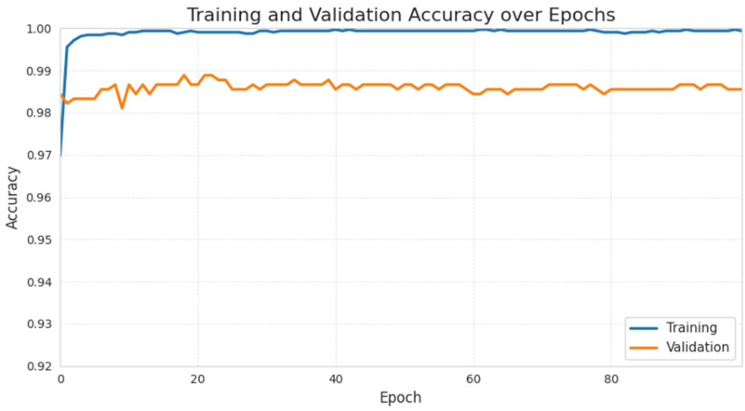
A training and validation accuracy graph over 100 epochs is presented in Figure 3. Both training accuracy and validation accuracy increased during the first few epochs before plateauing for the remainder of training. Specifically, training accuracy steeply increases in the first 10 epochs, from around 97% to 99.8%, and plateaues at around 99.7% to 99.9% for the next 90 epochs.

Validation accuracy also follows the same pattern as training accuracy with a slight increase in the initial 10 epochs. It then fluctuates mildly between 98.5% and 98.8% in the next 90 epochs.

These trends indicate that the model learns efficiently in the early stages and plateaus in performance in the rest of training.

The training precision stays high throughout the course of training, at around 99.9% to 100%. Similarly, validation precision also stays decently high throughout training, increasing from around 98.4% to 98.82% in the first 25 epochs before fluctuating slightly at around 98.6% to 98.8% in the next 75 epochs.

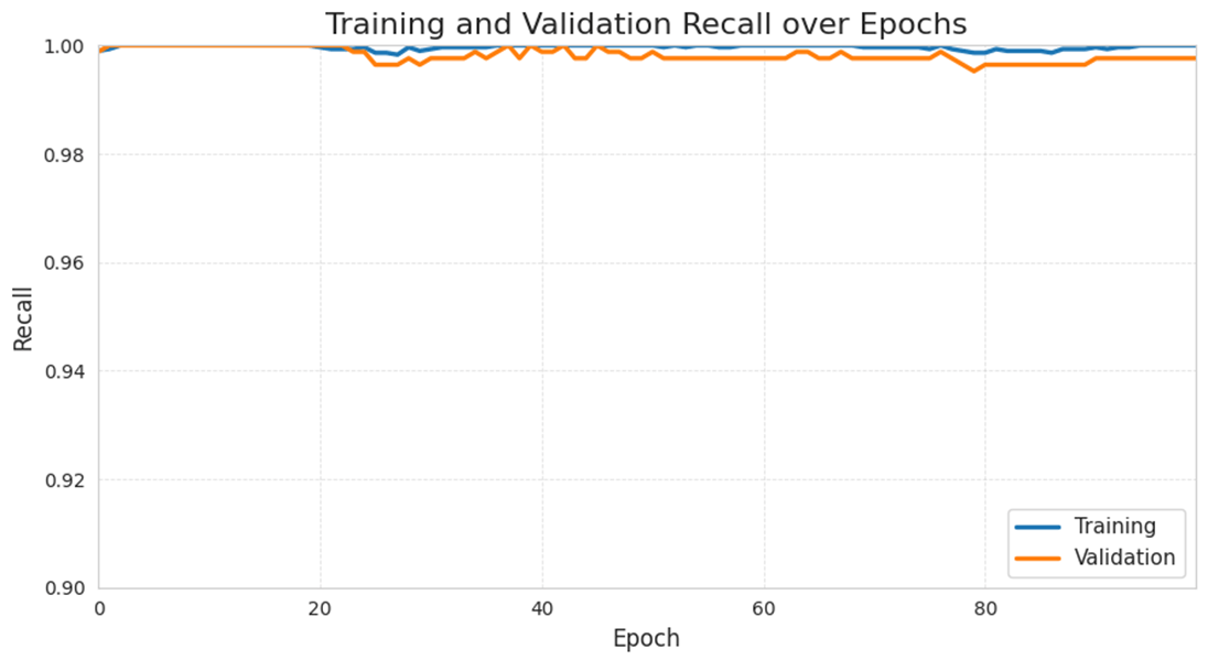
Similar to training precision, the training recall value also stays very high throughout training, always at around 99.8% to 100%. The model’s validation accuracy follows a similar trend, staying relatively high over the 100 epochs and fluctuates at around 99.52% to 99.9%. The high recall value shows that the model is strong in predicting positive events, suggesting a low the number of false negatives.

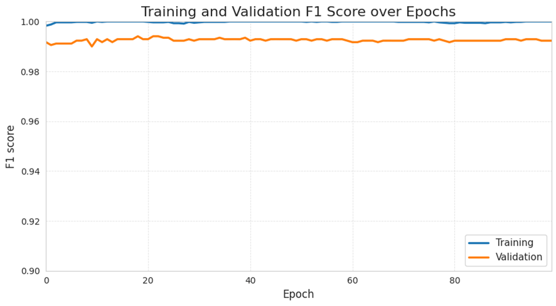
The F1 curves mirror the trends of recall and precision: training F1 and validation F1 stays relatively high throughout training, with little fluctuation. Specifically, the training F1 score stays at around 99.8% to 100% while the validation F1 score fluctuates between 99.1% to 99.3%. The training and validation F1 curves are close, showing a balanced precision and recall behaviour on the validation set.

In contrast, the ROC-AUC trend is way less consistent. The training ROC-AUC stays at 100% across the 100 epochs. Validation ROC AUC however, drops from 99.4% to 88.2% in the first 10 epochs before increasing to 93.78% at epoch 30. From epoch 31 to 100, it fluctuates at around 90% to 94%. Although the precision and recall values are very high, the ROC AUC is noticeably lower and more variable. It implies that the model had some level of overfitting during training: the model performs nearly perfectly on the training set but is more sensitive to noise in the validation set.

For the second tuning approach, which used a progressively decreasing number of neurons per layer (i.e., 32, 16, 8, 4), the best-performing configuration yielded a marginally lower validation accuracy of 98.77%. Thus, the uniform-layer model was thus selected for final testing.

In addition to neural networks, several other algorithms were evaluated for comparison. 

Firstly, Multiple Linear Regression was implemented as a baseline model, resulting in a Mean Squared Error (MSE) of 0.10431, which is a decently low Mean Squared Error for a linear model but it still has a lower accuracy than classification-based models. 

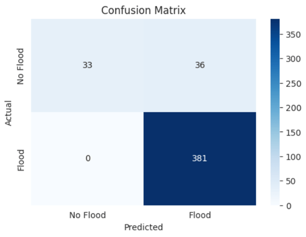
Secondly, Logistic Regression was tested and achieved 98.66% validation accuracy, demonstrating a strong performance with significantly faster training time and simpler architecture. Further evaluation of the performance of the Logistic Regression model is shown in the confusion matrix (Figure 8). It accurately predicted 33 cases of No Flood and 381 cases of Flood, with 36 false positives and 0 false negatives.

Thirdly, a Random Forest Classifier was employed and achieved a 98.55% validation accuracy, which is slightly lower than the Logistic Regression model and the best-performing neural network model. This shows the potential of ensemble approaches for classification on environmental data. Further evaluation of the performance of the Random Forest model is shown in the confusion matrix (Figure 9). The model correctly predicted 35 cases of No Flood and 380 cases of Flood, with only 34 false positives and 1 false negatives.

The Random Forest Classifier’s impurity-based feature importances indicate that rainfall is the dominant flood predictor (≈ 29.0%), followed by minimum temperature (≈ 15.1%), cloud coverage (≈ 13.4%), bright sunshine (≈ 11.1%) and relative humidity (≈ 9.5%). Geographical features such as altitude or x coordinates only contribute modestly to the final result (< 5%), while the period of the flood event contributes negligibly (≈ 0.4%). The SHAP analysis of the neural network model also shows that rainfall (≈ 17.6%) and bright sunshine (≈ 17.1%) are the top predictors. The geographical features, however, played a more important role in the neural network model, with the Y coordinates, latitude, and longitude contributing 11.4%, 9.5%, and 9.0% respectively. Some features, such as cloud coverage, minimum temperature, and relative humidity, played a less important role in the neural network model compared to the Random Forest Classifier. Overall, both methods consider rainfall as the most important factor, but the higher focus on spatial features of the neural network model indicates that the models differ in how local context is used.

Over a 5 time 5-fold cross-validation, the optimal neural network structure (the model with 6 layers of 60 neurons) outperformed the logistic regression model by 0.00913 in accuracy. This improvement is statistically robust: the paired t-test p-value is around 1.3×10^-11 and the Wilcoxon p ≈ 1.22×10^-5. Overall, the neural network model performed consistently better than the logistic regression across all folds.

After evaluating all the models, the neural network model with 6 layers of 60 neurons was chosen. To further evaluate the performance of that model, a 5-fold stratified cross validation was performed. The results of the cross validation are excellent: mean accuracy across 5 folds is 99.26% with a mean ROC-AUC of 99.84%, indicating the model has a strong ability to distinguish between classes. The precision (≈ 97.1%) and recall (≈ 98.1%) values are also high, giving an F1-score of around 97.55%. The variability of the values are also very low, with only precision having a standard deviation larger than 0.01 (≈ 0.016). Overall, these cross validation scores suggest very strong generalization on new and unseen data.

The post-hoc analysis revealed that many false positives occurred at stations with little to no rainfall, suggesting that the model might be missing some local predictor variables. Furthermore, the majority of errors occur for events after 2005, indicating that model performance degrades on later years. This pattern is consistent with changes in climate and the environment, suggesting the need for time-aware evaluation to enhance model performance.

On the measured hardware (Kaggle’s 2 NVIDIA T4 GPUs), training required 87.66 seconds wall time and 106.25 seconds Central Processing Unit (CPU) time. The mean inference speed averaged 0.094 seconds and corresponds to 0.208 milliseconds per sample or around 4802.83 samples per second. This makes the model fast enough for real-time flood forecasting.

Discussion

This study reaffirms that machine learning algorithms can successfully predict flood events when trained on large environmental data. The best performing neural network model, which had six hidden layers with 60 neurons in each, achieved a validation accuracy of 98.89%, followed by the funnel-shaped network achieved a validation accuracy of 98.77%. The logistic regression model achieved a 98.66% validation accuracy, the random forest classifier achieved 98.55%, and multiple linear regression attained an MSE of 0.10431. Furthermore, the Random Forest confusion matrix also contained only 34 false positives and 1 false negatives across nearly 450 validation cases, underscoring the power of ensemble methods.

An analysis of the flood occurrences from the Bangladesh dataset shows that flood incidence is heavily concentrated between June and September, which correlates with the monsoon months. Because the dataset records flood occurrences on a monthly basis and relies on news or national reports for labels, it can overlook some short-duration flash floods and events in sparsely populated or poorly monitored areas. Therefore, the model may be able to accurately predict monsoon-driven floods but might underperform when predicting micro-scale events.

These findings are important to the growing body of research on machine learning–based flood forecasting. By applying classification neural networks to a geographically extensive national dataset, this study confirms that accurate flood prediction is possible even in areas with complex climates. In contrast to previous research that depends on localized or river-specific information, the design of this model prioritizes generalizability—allowing adaptation to data-scarce regions that are susceptible to floods. The broad applicability across various environments serves to mitigate a significant research gap in literature where models are often either too specifically designed or require huge amounts of data. Additionally, the high validation accuracy indicates that even relatively straightforward architectures, when carefully adjusted, can equal more intricate alternatives. These findings are comfortably within this study’s initial research target: to develop a scalable and accurate prediction model using deep learning algorithms.

An important methodological choice in this study was lowering the neural network’s decision threshold from 0.5 to 0.3 to prioritize recall. In flood prediction, the consequences of false negatives are typically more damaging compared to false positives. False negatives can lead to insufficient safety measures, causing loss of lives, infrastructural damage. By contrast, false positives can result in false alarms and temporary evacuation, but its damage and cost is better than false negatives. Thus, the threshold adjustment is a necessary precaution to prioritize reducing false negatives in order to decrease the potential damage caused by floods.

In the future, several possibilities could further enhance and expand this work. The incorporation of human-infrastructure variables—such as urbanization, deforestation, and land use patterns—may reduce the residual error in some borderline cases. Including time-series inputs through recurrent or attention-based models could reflect temporal dynamics often preceding extreme events. Automated hyperparameter selection (e.g., Bayesian search) and stacked ensembles that combine neural networks, random forests, and logistic regression could improve the model’s performance with minimal tuning. In addition, automated threshold optimization methods – such as cost-sensitive thresholding or ROC Curve Analysis – could further refine the balance between the number of false negatives and false positives by tuning the decision threshold to reflect real-world misclassification.

Despite the strong performance of the model, there are six significant limitations that can influence the result. First, the dataset is dominated by environmental factors such as rainfall, humidity, and temperature, but no human and infrastructural variables. Variables such as urbanization, land use pattern, and population can significantly contribute to flood behavior in urban or populous areas. Without such characteristics, the model could lack crucial context relevant to occurrences of floods. To address these limitations, future work can augment the dataset with human and infrastructure-related data from various public sources – for example, census or population maps, OpenStreetMap for data on roads and drainage systems, and satellite imagery – and combine them accordingly with the environmental data based on time and location. This data can give the model important context about where people and infrastructure can affect flood risk and its potential damage. These richer inputs can then be processed using multi-modal models (models that can process image and tabular time-series inputs) which can improve its performance by considering more flood-related variables and make predictions more useful for planning and response. Second, the dataset contains high collinearity among some variables (e.g., such as rainfall vs. flood, longitude vs. X coordinate) as demonstrated in the correlation heatmap. Having such high correlation between the variables can lead to unnecessary computations and distorts the variance of the model’s coefficients. This study did not implement feature selection or dimensionality reduction techniques to mitigate this limitation. Addressing this limitation in future work – such as implementing regularization (Lasso or Ridge), Principle Componenet Analysis (PCA), or analyzing the correlation heatmap – can reduce unnecessary variables and enhance the model’s stability and performance. Third, although the dataset consists of an extensive number of flood events, it has substantial class imbalance (4,132 flood events versus 361 no flood events). Such an imbalance can lead the model to predict flood conditions more accurately, potentially underestimating vital flood events. Methods such as synthetic oversampling (Synthetic Oversampling Minority Technique (SMOTE) or Adaptive Synthetic Sampling (ADASYN)), class-weighted loss functions, and cost-sensitive training can reduce the model’s bias and recall/precision tradeoffs. Therefore, implementing these methods in future studies can help reduce bias towards the majority class and provide a fairer assessment of the model’s performance. Fourth, the time range of the dataset spans from 1948 to 2013. While it does provide data on long term environmental trends, it undermines the recent climatic patterns and the increasing number of extreme weather events over the past decade due to climate change⁸, limiting the model’s sensitivity to present-day risks. Furthermore, this study’s model treats each monthly label as a static input rather than modeling temporal sequences. Time series models such as long short-term memory (LSTM) or gated recurrent unit (GRU) could help capture these seasonal and temporal dynamics which are important flood factors. Fifth, this study overlooked alternative deep learning structures, such as 1D convolutional neural networks (CNN) for time-series data and recurrent neural networks, which could help put the feed-forward neural network’s performance into a broader context. Lastly, the dataset has a limited geographical scope. Although the dataset covers a wide range of environmental conditions within Bangladesh, its scalability to global contexts – particularly regions with vastly different climates, landforms – remains uncertain. In addition, monthly label granularity and event reporting biases may overstate the overall accuracy and overestimate the true accuracy of under-represented, minor events. These limitations leave scope for further work to extend the dataset and fairness to the model.

Overall, this study demonstrates that machine learning models—when optimized using vast, high- quality datasets—can reliably predict nearly 99% of flooding incidents. With further tuning of the model inputs and architectures, it is becoming increasingly feasible to approach real-time, reliable early-warning systems that are able to prepare societies and mitigate the impacts of one of nature’s most destructive forces.

All codes, preprocessing scripts, trained model weights, and the dataset used in this study are available at the Github repository in the Reference section.

References

1. World Vision. Floods Facts & FAQs: How to Help. World Vision (2025). https://www.worldvision.org/disaster-relief-news-stories/floods-facts-faqs-how-to-help  [↩]
2. Konrad, Christopher P. Effects of Urban Development on Floods. Fact Sheet FS-076-03, U.S. Dept. of the Interior, U.S. Geological Survey (2003). https://doi.org/10.3133/fs07603 [↩]
3. World Meteorological Organization. Floods. WMO (2025). https://wmo.int/topics/floods [↩]
4. Soil & Water Assessment Tool (SWAT). Texas A&M AgriLife Research (n.d.). https://swat.tamu.edu [↩]
5. Mosavi, Amirreza, Pooyan Ozturk, Ka Chun Chau, and Yahya Salhi. Flood Prediction Using Machine Learning Models: Literature Review. Water 10 (11) 1536 (2018). https://doi.org/10.3390/w10111536 [↩]
6. Shi, Jimeng, Zeda Yin, Rukmangadh Myana, Khandker Ishtiaq, Anupama John, Jayantha Obeysekera, Arturo Leon, and Giri Narasimhan. Deep Learning Models for Flood Predictions in South Florida. arXiv preprint arXiv:2306.15907 (2023). https://doi.org/10.48550/arXiv.2306.15907 [↩] [↩]
7. Gauhar, Noushin and Das, Sunanda and Moury, Khadiza Sarwar. Prediction of Flood in Bangladesh using k-Nearest Neighbors Algorithm. Github (2021). https://github.com/n-gauhar/Flood-prediction [↩] [↩]
8. BBC News. Climate change: Extreme weather events ‘have increased’. BBC News (2021). https://www.bbc.com/news/science-environment-58396975 [↩]