
Abstract
This study looks at the effect of Twitter Sentiment on stock returns. With a focus on Apple Inc., we aim to understand how social media influences the stock market over a short period of time (1, 2, 3, and 7 days after the tweet was posted). We utilized a dataset containing 862,321 labelled tweets, the stock returns of the targeted company, and the sentiments of each tweet to create Random Forest and Linear Regression models. We continued with Random Forest as it produced the best results, and we fine-tuned the 10 models created. Our results revealed that model 10 (using tweet polarity and the stock returns 1, 2, and 3 days after the tweet was posted to predict the return after 7 days) obtained the highest  score of 0.996 while also having a near negligible Mean Squared Error value. Features such as stock returns and tweet sentiment we essential to our investigation, and we also conducted a SHAP analysis to determine the marginal contribution of each feature on the models’ predictions. Our results reveal that the polarity of a tweet does not have a significant effect on the predictions made by our models. Rather, it is the stock returns of the previous time interval that greatly contribute to their predictions. Though this was revealed, combining both historical data and tweet/social media sentiments could still improve the accuracy of models designed to predict stock returns and stock market fluctuations. Future research could investigate different industries to examine its applicability on a broader scale.
Introduction
The relationship between stock market movements and social media sentiment has been increasingly recognized in Behavioral Finance Theory. Although most traditional financial models place reliance on the Efficient Market Hypothesis, which states that all share prices reflect all available information1, Behavioral Finance Theory acknowledges that investor decisions can be influenced by biases and psychological influences2, which could – in turn – stimulate market movements.
Multiple instances have shown how certain tweets can affect their targeted stock’s returns. For example, Elon Musk in 2018 (whose tweet caused Tesla’s stock price to increase by 6%)3 ) and Donald Trump in 2017 (whose tweet caused Amazon’s stock market valuation to drop by USD$5bn)4. It is instances like these that show us that stock prices are not solely influenced by data like financial statements (such as a firm’s profits, costs and revenue) or economic indicators (such as a firm’s growth), but investor sentiments as well.
The theorical foundation of study is grounded in Behavioral Finance Theory, which states that participants’ cognitive biases can lead to deviations from rational pricing5. Social media platforms such as Twitter serve as a real-time measure of the mood of the public, and utilizing ML to understand the impact of twitter sentiment analysis on stock prices allows for data analysis to find the correlation between these variables as well as providing useful insights into market inefficiencies, offering new opportunities for investment and trading tactics. Dedicating this study to Apple Inc.’s stock could limit the generalizability of our models on a broader perspective, as different industries or companies may be affected differently.
Multiple studies have been conducted in the past to provide valuable insights about predicting stock returns using a twitter sentiment analysis, and their correlation. A paper by Christian Palomo6 focused on developing an NLP model to predict certain stock prices by directly analyzing the sentiment of a tweet using a transformer based neural network, a method that differs greatly from traditional Machine Learning and Natural Language Processing techniques. Palomo’s work utilized the dataset Twitter-Financial News Sentiment from the HuggingFace website, containing 12,424 entries of finance-related tweets. Each entry had been split into three categories based on whether the tweet corresponds to an increase in stock price, a decrease in stock price, or neither. Multiple models for specific months were created and tested. The model developed in this study aimed to predict the stock movements of Tesla from August 2022 through December 2022. The model’s results from November 2022 had an accuracy of 82%, with its predictions matching the stock movements of 19 out of the 22 days the market was open for.
Moreover, Anshul Mital and Aprit Goel7 had conducted a similar study in which they aimed to find the correlation between public and market sentiments. Mital and Goel targeted values from the Dow Jones Industrial Average (DJIA) from June 2009 to December 2009, obtaining their data from Yahoo! Finance (containing the opening prices, closing prices, as well as the highest and lowest prices) and publicly available Twitter data (containing more than 476 million tweets including the timestamp, username and tweet text). Mital and Goel preprocessed their data by utilizing a concave function ( (y+x)/2: where x is the DJIA value on a given day, and y is the next available data point with n number of days between x and y), adjusting stock values by shifting prices up/down for jumps/falls with a large magnitude, and removing periods of significant volatility to prune their dataset. Next, a sentiment analysis of tweets was conducted, classifying tweets as either positive or negative. However, Mital and Goel also used a much lesser-known form of classification: multi-class classification, in which they used four mood classes — Calm, Happy, Alert, and Kind. Mital and Goel then finished preprocessing their data by generating a word list (based on the Profile of Mood States), filtering tweets, computing a daily score for every POMS word on a given day, and mapping those scores. To train and test models, Mital and Goel used four different algorithms: Linear Regression, Logistic Regression, SVMs and Self-Organizing Fuzzy Neural Networks (SOFNNs). The accuracies of these models were derived using k-fold sequential cross validation where k was 5. The results documented in this study show that the SOFNNs performed the best out of the four algorithms with an accuracy of around 75.56%.
The objective of this study is to understand the effect of tweets on their targeted stock’s price. Additionally, we investigate how long, if any, the effect of the tweet lasts and/or impacts the stock price into the near future.
Dataset & Ethical Considerations
Although data obtained from Twitter is publicly available, it is still important to ensure that privacy requirements are met as there may be certain individuals who would not expect their tweet to be used in a study. Our study follows the ethical guidelines below:
- We ensured that user identity remained anonymous by using Tweet Sentiment’s Impact on Stock Returns as our dataset. This dataset does not contain any personally identifiable information.
- We consider any potential biases prevalent in data from social media and how they impact our analysis
- Our findings are presented with appropriate cautionary notes about how they could potentially be misused for market manipulation
- We acknowledge that users on Twitter may not have expected their tweets to be used in our analysis
Tweet Sentiment’s Impact on Stock Returns can be accessed from Kaggle8. It contains 862,231 labelled tweets and their respective stock returns. Each tweet had their date of the tweet extracted as well as the company the stock is aimed at. Furthermore, all labelled tweets have been assigned a polarity (the tone of the tweet) that will aid the user in their analysis of the data using machine learning. Polarity is the sentiment expressed by a text, and can be positive, negative, or neutral9. To obtain a polarity, a sentiment analysis had been pre-applied. However, below is how sentiment analysis is typically done to obtain value for the tweet’s polarity:
- Tweets were tokenized and stop words were removed. The text was later lemmatized as per the NLP process
- LSTM Neural Networks and TextBlob were used to extract the sentiment of the tweets
- The polarity scores were then added into the dataset as features
Tweet Sentiment’s Impact on Stock Returns contains several columns affiliated with tweets and their targeted stock’s returns or losses. Every entry in this dataset contains the TWEET (The text of the tweet), the STOCK (stock mentioned in the tweet), and the DATE (The date at which the tweet was posted). Additionally, the dataset also contains the LAST_PRICE (The targeted stock’s price at the time of tweeting), PX_VOLUME (The volume of shares traded at the time of tweeting), VOLATILITY_10D and VOLATILITY_30D (The targeted stock’s volatility across a 10 and 30-day window), and 1_DAY_RETURN, 2_DAY_RETURN, 3_DAY_RETURN, and 7_DAY_RETURN (The returns of losses of the targeted stock 1, 2, 3, and 7 days after the tweet was posted). Finally, sentiment scores were calculated using two approaches:
- LSTM_POLARITY: Values in this column were derived from a long-short-term-memory (LSTM) neural network, a type of recurrent neural network (RNN) that can learn long-term dependencies – a problem that regular RNNs have10.
- TEXTBLOB_POLARITY: Values in this column were derived using the TextBlob lexicon-based method. TextBlob is a library for Natural Language Processing (NLP) and supports analysis and operation on textual data.
For clarity, we will be referring to these features as “LSTM polarity” and “TextBlob polarity” in this study. However, column headers from the dataset will keep their original name (LSTM_POLARITY, TEXTBLOB_POLARITY), with an exception to when we are explicitly mentioning the dataset’s features.
Results
| Model No. | Input Features | Target Output | Best Parameters | MSE (Train) | MSE (Test) | ||
| 1 | LSTM_POLARITY | 1_DAY_RETURN | max_features: 1, min_samples_split: 80, n_estimators: 500 | 0.001099 | 0.000166 | -0.000142 | 0.000224 |
| 2 | LSTM_POLARITY | 2_DAY_RETURN | max_features: 1, min_samples_split: 190, n_estimators: 500 | 0.0000077 | 0.000397 | -0.054058 | 0.000173 |
| 3 | LSTM_POLARITY, 1_DAY-RETURN | 2_DAY_RETURN | max_features: 1, min_samples_split: 10, n_estimators: 500 | 0.970368 | 0.942775 | 0.000012 | 0.0000094 |
| 4 | LSTM_POLARITY | 3_DAY_RETURN | max_features: 1, min_samples_split: 74, n_estimators: 500 | 0.000055 | -0.039843 | 0.000562 | 0.000433 |
| 5 | LSTM_POLARITY, 1_DAY-RETURN | 3_DAY_RETURN | max_features: 1, min_samples_split: 50, n_estimators: 500 | 0.944464 | 0.87072 | 0.000031 | 0.000054 |
| 6 | LSTM_POLARITY, 1_DAY-RETURN, 2_DAY_RETURN | 3_DAY_RETURN | max_features: 2, min_samples_split: 80, n_estimators: 500 | 0.986152 | 0.980537 | 0.0000078 | 0.0000081 |
| 7 | LSTM_POLARITY | 7_DAY_RETURN | max_features: 1, min_samples_split: 50, n_estimators: 500 | 0.017493 | -0.723959 | 0.00135 | 0.001036 |
| 8 | LSTM_POLARITY, 1_DAY-RETURN | 7_DAY_RETURN | max_features: 1, min_samples_split: 5, n_estimators: 500 | 0.876224 | 0.628146 | 0.00017 | 0.000223 |
| 9 | LSTM_POLARITY, 1_DAY-RETURN, 2_DAY_RETURN | 7_DAY_RETURN | max_features: 2, min_samples_split: 10, n_estimators: 500 | 0.956834 | 0.819039 | 0.000059 | 0.000109 |
| 10 | LSTM_POLARITY, 1_DAY-RETURN, 2_DAY_RETURN, 3_DAY_RETURN | 7_DAY_RETURN | max_features: 2, min_samples_split: 70, n_estimators: 500 | 0.999988 | 0.996942 | 0.000000016 | 0.0000018 |
SHAP Plots


| Model | R2 (Train) | MSE (Train) | R2 (Test) | MSE (Test) |
| Model 10 (Table 1) | 0.999988 | 0.000000016 | 0.996942 | 0.0000018 |
| Naïve Lagged Return | 0.099696 | 0.001268 | 0.244418 | 0.000357 |
| Historical Mean Return | 0.000000 | 0.001408 | -1.141211 | 0.001011 |
| Zero-Return | -0.347179 | 0.001897 | -0.002576 | 0.00473 |
Discussion
Model Results: Best Parameters, Train and Test MSE and R2 Values
In this section, we will be discussing the models developed in this study, their results, best parameters, and train and test R2 scores. We developed 10 models to take all possibilities into account, and we obtained their train and test R2 scores as well as MSE values. After that, we tuned the models and used GridSearch to find the best parameters. These will help us determine whether the models are able to make predictions using the provided input features.
Table 1 shows that models predicting a certain X_DAY_RETURN (Models 1, 2, 4, and 7) using LSTM polarity as its only input feature have extremely low training and testing R2 scores. The model predicting 2_DAY_RETURN using LSTM polarity as its only input feature had scores of
 and 0.000166 for the training and testing set respectively. Low R2 scores in models like these indicate that the model performs poorly when it comes to its predicting power, and they also indicate that these models were unable to explain the majority of variances within the dataset.
On the other hand, models that used multiple features such as model 10 (where LSTM polarity, 1_DAY_RETURN, 2_DAY_RETURN, and 3_DAY_RETURN were used to predict 7_DAY_RETURN) performed marginally better compared to models 1, 2, 4, and 7. Model 10 obtained a training R2 score of 0.999988 and a testing R2 score of 0.996942. These R2 scores indicate that model 10 was able to explain the variances within the dataset and make accurate predictions, while also having minimal overfitting and extremely low MSE values.
A similar pattern can be seen in model 9 (where LSTM polarity, 1_DAY_RETURN, and 2_DAY_RETURN were used to predict 7_DAY_RETURN). This model had a training R2 score of 0.956834 and a testing R2 score of 0.819039. These scores indicate that model 9 was able to make a significant number of accurate predictions during both training and testing. However, some overfitting was present, evident in the 14% decrease in R2 scores from training to testing. Nevertheless, the model still had considerably low MSE values during training and testing, indicating that the model can make good generalizations about the dataset.
While most models are able to make good generalizations about the dataset, some models still experience overfitting. One such model is model 8 (where LSTM polarity, and 1_DAY_RETURN were used to predict 7_DAY_RETURN), which obtained a training R2 score of 0.876224 and a testing R2 score of 0.628146. The variance of these scores indicates some overfitting and shows that model 8, while still being able to make some generalizations, was unable to make generalizations to the same degree of accuracy as it did during training, suggesting that it may have learnt the patterns in the training set a little too well, causing it to perform worse during testing.
To ensure that overfitting is mitigated in future studies, many techniques can be implemented.
Feature reduction, through the use of Principal Component Analysis, can remove features that have a low importance relative to the dataset’s other features which would prevent the model from learning with the noise in the data. Furthermore, regularization techniques such as Lasso (L1) – which shrinks the coefficients of unnecessary features to 0 by adding a penalty term to the usual Squared Error function (resulting in the function  – and Ridge (L2) – which also adds a penalty , but for the purpose of reducing the importance of certain features (resulting in the function
  ) –11 can reduce the risk of the model memorizing patterns instead of learning them. Additionally, cross-validation methods such as the time-series cross-validation could further improve the model’s predictive accuracy by having each fold use past data for training and future data for testing, which differs from the random shuffles that traditional cross-validation uses12. Moreover, simply re-running models with higher min_sample_split values – that start at 60, 70, or even 80 – may reduce the model’s overfitting.
SHAP Analysis
We conducted a SHAP analysis to determine the impact that the dataset’s features have on our model’s predictions of stock returns after a certain number of days the tweet was posted. Using a SHAP analysis is an integral part in finding out how much each feature contributes to the model’s predictions. SHAP is based on Shapley Values, a game theory framework developed by Lloyd Shapley, and can be used to interpret any type of machine learning model13. Features with a positive SHAP value will positively affect the model’s prediction, and vice versa for features with a negative SHAP value. Every feature in the SHAP analysis is given an importance value which represents that feature’s contribution to the model’s output, doing so allows for the calculation of the extra contributions made by each feature.
Conducting a SHAP analysis of features will allow us to visualize the contributions made by features. This is extremely important, especially when the model’s results are unexpected. A SHAP analysis will help us find the features that made the most contributions to a model’s prediction, and features that made the least contributions: this analysis may help us identify whether LSTM polarity has an impact on the model’s predicted stock returns. We analyzed the SHAP plots for the models that predict 7_DAY_RETURN (models 7-10) because these models were the ones that performed relatively better compared to the other models.
Figure 1 displays the SHAP plots of model 7 (where the input feature is LSTM polarity, and the target output is 7_DAY_RETURN). The summary plot shows us that higher LSTM polarity values (red) are pushing the model’s predictions towards negative values, and lower LSTM polarity values (blue) are pushing the model’s predictions towards positive values. The bar plot shows us that the average SHAP value for LSTM polarity is slightly greater than 0, indicating that the feature has a small but positive effect on the target output. Figure 1 revealed that LSTM polarity does not have a major impact on the model’s predictions.
Figure 2 displays the SHAP plots for model 8 (input features for this model are LSTM polarity and 1_DAY_RETURN, and the target output is 7_DAY_RETURN). The summary plot shows us that higher LSTM polarity values slightly push the model’s predictions to the left, and lower LSTM polarity values slightly push the model’s predictions towards the right, indicating that LSTM polarity has a small impact on the model’s predictions. Moreover, the plot also shows us that some higher and lower 1_DAY_RETURN values can push the model’s predictions to the right, and some can also push the model’s predictions towards the left. The bar plot shows us that 1_DAY_RETURN has a much larger impact on the model’s predictions compared to LSTM polarity. It shows us that 1_DAY_RETURN increases the model’s predictions by 0.02 on average, whereas the contributions made by the LSTM polarity are almost negligible.
Figure 3 displays the SHAP plots for model 9 (where the input features are LSTM polarity, 1_DAY_RETURN and 2_DAY_RETURN, and the target output is 7_DAY_RETURN). The summary plot shows us that contributions to the model’s predictions by LSTM polarity are almost negligible, and that compared to Figure 2, 1_DAY_RETURN’s contributions seem to have decreased. Nevertheless, both high and low values of this feature push the model’s predictions to the left, and some push the model’s predictions to the right. The summary plot also shows us that 2_DAY_RETURN has the biggest impact on the model’s predictions, and that higher values for this feature positively impact the model’s predictions, and vice versa for lower values. The bar plot shows us that 2_DAY_RETURN increases the model’s predictions by 0.02 on average, 1_DAY_RETURN increases the model’s predictions by 0.01 on average (lower than the value displayed in Figure 1), and LSTM polarity has a near negligible effect on the model’s predictions.
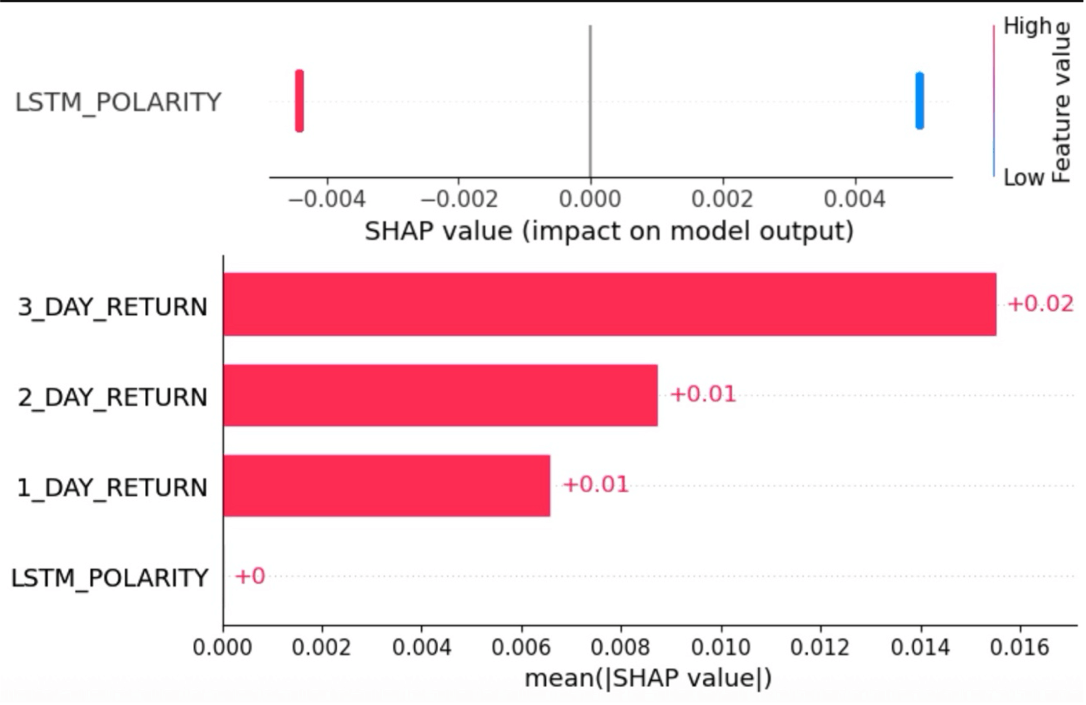
Figure 4 displays the SHAP plots for model 10 (where the input features are LSTM polarity, 1_DAY_RETURN, 2_DAY_RETURN and 3_DAY_RETURN, and the target output is 7_DAY_RETURN). The summary plot shows us that 3_DAY_RETURN had the largest contribution to the model’s predictions, with higher values of this feature positively impacting its predictions, and vice versa for lower values. 2_DAY_RETURN has similar results to that of 3_DAY_RETURN. However, for 1_DAY_RETURN, it appears as if higher values of this feature are influencing the model’s predictions to a higher degree compared to lower values of this feature, and LSTM polarity seems to have the smallest contribution out of the four input features. The bar plot shows us that 3_DAY_RETURN increases the model’s predictions by 0.02 on average (a noticeable trend is that the greatest X_DAY_RETURN seems to increase the model’s predictions by 0.02 on average). It also shows us that 1_DAY_RETURN and 2_DAY_RETURN increase the model’s predictions by 0.01 each, and that LSTM polarity has a negligible contribution.
In summary, the SHAP values from Figures 1-4 show us that historical stock returns from 1-3 days since the tweet was posted were the most dominant predictors, and that the LSTM polarity feature of each data entry played a minimal role. These findings provide practical and valuable insights for market participants:
- Portfolio managers could use returns from 1–3-day intervals as key signals but can also make use of social media sentiment as a means of secondary confirmation.
- Traders can utilize the non-linear relationship revealed by our SHAP values to create new strategies or refine existing ones to maximize profit
- Risk analysts can use social media sentiments as warnings for possible overreactions (herd behavior, panic buying/selling, confirmation biases). However, our results caution against the overuse of these sentiments.
However, we believe that the tweet sentiments had negligible effects because of various reasons:
- Stock prices have a chance to react to investor sentiment with a delay. This would make it difficult for a model trained on stock movements ranging from 1-7 days after a tweet was posted. Should sentiment-driven movements occur with a delay, the period that the dataset covers may not show us that tweet sentiments and stock movements have a strong correlation
- Although tweets can target a certain company, not all tweets are relevant to stocks or stock price movements. If the majority of tweets come from those just casually tweeting about the company instead of experts in the finance sector, then the sentiment of the tweet may provide minimal contribution.
- Twitter sentiments as a feature might be overshadowed by other features such as historical stock returns (X_DAY_RETURN) as those features might simply be stronger predictors. If past data can already be used to explain – and even predict – variations in stock returns, tweet sentiments may not be able to contribute as much to the model’s predictions.
- Tweet polarity may not even be a good indicator or an accurate numerical representation of tweets. The use of more sophisticated Natural-language-processing (NLP) numerical representations such as BERT (Bidirectional Encoder Representations from Transformers) – which can help establish context –14 could possibly be a more viable option.
Naïve Model Comparisons
Our model 10 (Table 1) obtained an exceptional testing  score of 0.996942 and a MSE of
  , but we would like to contextualize these results by comparing them to our naïve models (Table 2):
- Naïve Lagged Return: In reference to Table 2, the naïve lagged return model had a testing score of 0.244418 and a testing MSE value of
 . This model can explain 24% of the variance in Apple’s 7-day-returns by using its returns over a 3-day period. This confirms the presence of short-term momentum. However, model 10 heavily improves on this by achieving a 99.5% reduction in prediction errors (model 10’s MSE of versus the naïve lagged return’s MSE of ). This shows us that combining tweet sentiments and stock returns over multiple days yields much better results, and that machine learning models will be able to capture complex relationships and dependencies that go beyond short-term momentum.
 - Historical Mean Return: The historical mean return model had a testing score of -1.141211 and a testing MSE value of 0.001011. The negative score of this model (as well as the magnitude) suggests that it was a catastrophic failure (with a 550x worse MSE value compared to model 10). This rules out the possibility of using mean-reversion tactics when testing and predicting stock returns, which underscores the trending nature of Apple Inc.’s stock price.
- Zero-Return Prediction: The zero-return model had a testing score of -0.002576 and a testing MSE value of 0.00473. This suggests that holding onto stocks underperforms our approach by 3 orders of magnitude in MSE (model 10’s versus the zero-return model’s 0.00473).
These findings not only demonstrate how combining tweet sentiments and historical data perform marginally better compared to naïve strategies, but they also reveal that Apple Inc.’s stock had directional trends and non-zero returns during the testing period.
Practical Implications
These findings underscore the potential of incorporating social media sentiments with historical financial data to enhance the accuracy of models designed to predict stock movements and returns. As the influence of technology on financial markets increases, the ability to employ real-time public sentiments will only be offering more promising applications for financial analysts, traders, and researchers.
From a practical perspective, our findings suggest that while historical stock returns are the dominant predictors of future stock returns, social media sentiments may still be able to provide value in the following scenarios:
- As a warning system for sentiment extremes that could come before any major price movements.
- When social media sentiments are combined with other indicators of stock price movements. Our results show us that social media sentiment alone cannot be used to predict stock returns and thus cautions against the over-reliance on this one indicator. Rather, it suggests that tweet sentiments can complement already existing indicators.
Methods
Input Features and Target Output
We filtered the dataset to tweets related to Apple Inc. This was done to ensure that any extra noise was left out, allowing for a more in-depth analysis of the relationship between tweets and a certain company’s stock returns.
Next, we created multiple models using 1_DAY_RETURN, 2_DAY_RETURN, 3_DAY_RETURN, 7_DAY_RETURN, and LSTM_POLARITY, as shown in Table 2. We started off by giving the X-column 1 feature: LSTM_POLARITY and giving the Y-column the 7_DAY_RETURN feature. Then, I created another model by adding 1_DAY_RETURN to the X-column. The process was repeated for 7_DAY_RETUTN until the features had the LSTM_POLARITY feature and the X_DAY_RETURN of the days less than the X_DAY_RETURN in the Y-column. This was repeated for 1_DAY_RETURN, 2_DAY_RETURN, and 3_DAY_RETURN. This ensured that all possibilities were accounted for, allowing for a better analysis of results.
| Model No. | Input Features | Output Target |
| 1 | LSTM_POLARITY | 1_DAY_RETURN |
| 2 | LSTM_POLARITY | 2_DAY_RETURN |
| 3 | LSTM_POLARITY, 1_DAY_RETURN | 2_DAY_RETURN |
| 4 | LSTM_POLARITY | 3_DAY_RETURN |
| 5 | LSTM_POLARITY, 1_DAY_RETURN | 3_DAY_RETURN |
| 6 | LSTM_POLARITY, 1_DAY_RETURN, 2_DAY_RETURN | 3_DAY_RETURN |
| 7 | LSTM_POLARITY | 7_DAY_RETURN |
| 8 | LSTM_POLARITY, 1_DAY_RETURN | 7_DAY_RETURN |
| 9 | LSTM_POLARITY, 1_DAY_RETURN, 2_DAY_RETURN | 7_DAY_RETURN |
| 10 | LSTM_POLARITY, 1_DAY_RETURN, 2_DAY_RETURN, 3_DAY_RETURN | 7_DAY_RETURN |
In addition to tweet sentiments, future works – or extensions of this study – could delve into other tweet-derived features such as tweet volume (frequency of mentions), user influence (verified accounts, celebrities, public figures), and the time at which the tweet was posted (pre-market against post-market hours). These additions could reveal more about the influence of social media on stock returns and can help us capture additional dimensions of social media sentiment.
Baseline Model Comparisons
To further examine our model’s performance, we evaluated the following benchmarks for each target output:
- Naïve lagged return: These models will predict each day’s return by using the previous day’s actual return (
 ). The models will operate on the basis that the previous day’s return will be the same as the next day’s return.
 - Historical mean return: These models will predict each day’s return by using the average return it observes while training (
 , where
  is the past returns in the training data, and N is the number of observations).
 - Zero-return prediction: These models will predict each day’s return by simply assuming that the stock price will remain unchanged compared to the previous day. Hence, the return would be 0. This represents the tactic to do nothing and hold shares.
These models were then evaluated using time-series splits as well as R2 and MSE. Their performance gives us context for interpreting our results from models that used tweet polarity – especially for discerning whether the combination of tweet sentiment and historical data have an advantage over naïve strategies.
Train-Test Split
Developing any type of machine learning model involves splitting the data into training and testing data. The model developed in this study utilized a time-series train-test split instead of the more conventional random train-test split15. We had initially split the data using the train-test split function. However, we realized that there were multiple tweets posted on the same day. This became a problem as it provided the model with some of the values it needed to predict in during its training process (data leakage), resulting in testing accuracies being unusually high without the model being able to fully learn about the relationships between variables. To address this, we implemented a time-series train-test split, which ensures that we adhere to the chronological order of the data entries. This means that tweets posted on the same day will be grouped together into either the training or testing sets instead of being put into both. This prevents data leakage while training the model and is a better representation of real-world scenarios, where past data is used to predict the future. Unlike a random train-test split, a time-series train-test split can provide much more realistic evaluations of our models’ performances and makes sure that their predictions are not from future data.
Hyperparameter Tuning & Evaluation Metrics
After splitting the model, we implemented linear regression and Random Forest baseline models. Random Forest is a supervised-learning algorithm that utilizes an ensemble learning method for regression. The tool obtains its results by creating several decision trees (each tree makes its own predictions) and creates an output by using either the mode of the classes, or the mean prediction for classification and linear regression respectively16. Random forest has several parameters that can be fine-tuned to ensure that the model outputs the highest possible score. We chose to tune max_features, min_samples_split, n_estimators and max_depth. max_features regulates the maximum number of features a given decision tree is allowed to use in order to make a prediction. n_estimators is the number of decision trees used in the random forestmodel. min_samples_split is used to define the minimum number of samples required to split a node in a random forest. max_depth defines the depth of each decision tree in the forest17.
We decided to select random forest as our primary model not only because its baseline model performed better, but because its multiple decision trees make it a much stronger model when it comes to capturing non-linear relationships such as the relationship between tweet sentiments and stock returns due to its lack of sensitivity to any outliers.
After developing a baseline random forest model, we tuned it using a GridSearch approach — a process where we alter the values of the chosen parameters to get the best possible result. GridSearch is an optimization function that tries every combination using the provided parameter values to find the best model18. We decided to use GridSearch to explore the following parameters:
- min_samples_split: 10 to 200: We set the minimum samples needed to split a node between 10 and 200 to reduce any overfitting due to noise with values less than 5, and to prevent the creation of overly coarse splits with values greater than 200. These values are also incremented by 5
- max_features: 1 to n_features-1: We set the maximum number of features between 1 and 1 minus the total number of features so that we can figure out the optimal combination of features and the trade-off between predictive power and feature diversity
- n_estimators: 500: We set the number of trees in the random forest to 500 as we believed it to be a suitable amount to ensure that the model doesn’t plateau, while also ensuring that the process is conservative
- max_depth: 5-30: We set the maximum depth of each decision tree between 5 and 30 as values below 5 can risk underfitting, so the model would not be able to capture relationships. Values above 30 risks overfitting but also makes the process more computationally intensive, which is why we set our maximum as 30.
We specified the scoring to be R2 and the cv (cross-validation strategy) to be the time-series split. Overall, these parameters were chose to optimize efficiency and performance given the size of our dataset.
We used and mean-squared error (MSE) as our evaluation metrics for this study, and we compared the training scores to the testing scores of the evaluation metrics to determine whether the models were being overfitted. is used to determine the proportion of variance in the target output, measure how well it can predict outcomes in the future and reflect how well a model fits the dataset on a scale of 0 to 1, with larger values of indicating a better fit and smaller values indicating a worse fit. The value of can be obtained using the formula  19 where SSE is the sum of squares of errors (sum of squared differences between training and testing values) and SST is the total sum of squares (sum of squared differences between individual training values and the mean of the training values).
MSE is a loss function and measures the average of squared differences between the model’s predictions and the actual values of those predictions. A lower MSE indicates that the model’s predictions are getting close to the actual values and vice versa for a higher MSE. Values for this loss function can be obtained using the formula  where n is the number of data points, i is the index value of each data point,
  is the actual value of the ith data point, and
  is the model’s prediction of the ith data point20. It is important to note that MSE places a bigger weight on larger differences because it takes its square, making the function sensitive to outliers in the dataset.
Conclusion
This study aimed to understand the effects of tweets on their targeted stock’s returns, and how long these effects lasted for. We developed various machine learning models to explore this relationship, and we used the features provided in the dataset (LSTM_POLARITY, 1_DAY_RETURN, 2_DAY_RETURN, 3_DAY_RETURN, and 7_DAY_RETURN). We also filtered our dataset to specifically target tweets related to Apple to ensure that our analysis would be as accurate as possible
Using the previously mentioned scores, values and parameters, we concluded that model 10 (input features were LSTM_POLARITY, 1_DAY_RETURN, 2_DAY_RETURN, and 3_DAY_RETURN, and the target output was 7_DAY_RETURN) had performed the best (see table 2) and had obtained scores of 0.999 and 0.996 for training and testing respectively. We believe that this may have occurred because this model had the greatest amount of input features, thus feeding the model more information to help it find patterns and make generalizations about the dataset.
Finally, we conducted a SHAP analysis of models 7-10 to understand the marginal contributions of the input features on the model’s predictions. These plots showed us that LSTM_POLARITY had a negligible effect on the model’s predictions, with the other input features having a much more significant contribution. This is also evident in the models’ results, as models with LSTM_POLARITY as their only input feature had obtained scores that were close to 0. We also realized that adding features such as 1, 2 and 3 day returns significantly improved prediction accuracies.
In order to assess the generalizability of our study beyond Apple Inc., we propose that future studies should look at sectors with the following traits:
- High volatility: Industries that tend to have very high volatility – such as cryptocurrencies – may have stronger correlations to tweet/social media sentiments as opposed to stable industries such as healthcare.
- Retail investor participation: Companies that have a high retail ownership (a large portion of a company’s shares are held by individual investors instead of larger entities) can be much more susceptible to social media sentiment. In 2021, retail traders coordinated a short-squeeze to drive up the price of GameStop’s (GME) shares because they believed that GameStop was undervalued. As a result, posts such as “GME TO THE MOON” went viral21, leading to GameStop’s share price moving from
 86 in less than a month22.
Conducting future studies can provide researchers with an even better understanding on how public sentiments can be used to enhance decision-making in multiple market conditions, potentially reforming investment tactics in a digital landscape that is only going to keep evolving.
References
- Downey, L. (no date) Efficient market hypothesis (EMH): Definition and critique, Investopedia. Available at: https://www.investopedia.com/terms/e/efficientmarkethypothesis.asp (Accessed: 04 May 2025). [↩]
- Hayes, A. (no date) Behavioral finance: Biases, emotions and financial behavior, Investopedia. Available at: https://www.investopedia.com/terms/b/behavioralfinance.asp (Accessed: 04 May 2025). [↩]
- E. McCormick. Tesla trial: Did Musk’s tweet affect the firm’s stock price? Experts weigh in. The Guardian, 29 January. https://www.theguardian.com/technology/2023/jan/28/tesla-trial-elon-musk-what-you-need-to-know-explainer (2023, accessed October 16, 2024 [↩]
- The Guardian. Amazon stock market value falls by $5bn after critical Trump tweet. The Guardian, 16 August. https://www.theguardian.com/us-news/2017/aug/16/trump-amazon-taxes-tweet (2017, accessed October 16, 2024). [↩]
- Hayes, A. (no date) Behavioral finance: Biases, emotions and financial behavior, Investopedia. Available at: https://www.investopedia.com/terms/b/behavioralfinance.asp (Accessed: 04 May 2025). [↩]
- C. Palomo. Tweet sentiment analysis to predict stock market. CS224N, Stanford University. https://web.stanford.edu/class/archive/cs/cs224n/cs224n.1234/final-reports/final-report-170049613.pdf (2023, accessed August 31, 2024). [↩]
- R. Goel, A. Mittal. Stock market prediction using Twitter sentiment analysis. CS229, Stanford University. https://cs229.stanford.edu/proj2011/GoelMittal-StockMarketPredictionUsingTwitterSentimentAnalysis.pdf (2011, accessed August 31, 2024). [↩]
- Tweet sentiment’s impact on stock returns (no date) Kaggle. https://www.kaggle.com/datasets/thedevastator/tweet-sentiment-s-impact-on-stock-returns/data (accessed May 30, 2024). [↩]
- Prasanna, M.S.M., Shaila, S.G. and Vadivel, A. (2023) Polarity Classification on Twitter data for classifying sarcasm using clause pattern for sentiment analysis – multimedia tools and applications, SpringerLink. Available at: https://link.springer.com/article/10.1007/s11042-023-14909-w#:~:text=The%20text%20is%20categorized%20as,negative%20tweets%20for%20learning%20purposes. (Accessed: 04 May 2025). [↩]
- Group, I. (2020) Recurrent neural network and long term dependencies, Medium. Available at: https://infolksgroup.medium.com/recurrent-neural-network-and-long-term-dependencies-e21773defd92#:~:text=Long%20Short%20Term%20Memory%20networks%20(LSTMs)%20is%20a%20special%20kind,time%20is%20their%20default%20behavior. (Accessed: 05 May 2025). [↩]
- L1 and L2 regularization methods, explained (no date) Built In. Available at: https://builtin.com/data-science/l2-regularization#:~:text=Both%20L2%20regularization%20and%20L1,a%20generalized%2C%20less%20complex%20model. (Accessed: 05 May 2025). [↩]
- Shrivastava, S. (2020) Cross validation in Time Series, Medium. Available at: https://medium.com/@soumyachess1496/cross-validation-in-time-series-566ae4981ce4 (Accessed: 05 May 2025). [↩]
- A. A. Awan. An introduction to SHAP values and machine learning interpretability. DataCamp. https://www.datacamp.com/tutorial/introduction-to-shap-values-machine-learning-interpretability (2023, June 28). [↩]
- Hashemi-Pour, C. and Lutkevich, B. (2024) What is the bert language model?: Definition from TechTarget, Search Enterprise AI. Available at: https://www.techtarget.com/searchenterpriseai/definition/BERT-language-model#:~:text=BERT%20language%20model%20is%20an,surrounding%20text%20to%20establish%20context. (Accessed: 05 May 2025). [↩]
- M. En-nasiry. Time series splitting techniques: Ensuring accurate model validation. Medium. https://medium.com/@mouadenna/time-series-splitting-techniques-ensuring-accurate-model-validation-5a3146db3088#:~:text=TimeSeriesSplit&text=It%20divides%20your%20data%20into,in%20tscv.split(X)%3A (2024, June 21). [↩]
- A. Chakure. Random forest regression in Python explained. Built In. https://builtin.com/data-science/random-forest-python (2023, April 27). [↩]
- M. B. Fraj. In depth: Parameter tuning for random forest. Medium. https://medium.com/all-things-ai/in-depth-parameter-tuning-for-random-forest-d67bb7e920d (2017, December 21). [↩]
- Grid search. Dremio. https://www.dremio.com/wiki/grid-search/ (2024, July 16). [↩]
- E. Onose. R squared: Understanding the coefficient of determination. Arize AI. https://arize.com/blog-course/r-squared-understanding-the-coefficient-of-determination/#:~:text=The%20R%2Dsquared%20metric%20%E2%80%94%20R%C2%B2,be%20explained%20by%20your%20model (2023, August 8). [↩]
- Mean square error (MSE): Machine learning glossary. Encord. https://encord.com/glossary/mean-square-error-mse/ (no date). [↩]
- Volpicelli, G.M. (2021) This was the year when finance jumped the Doge, Wired. Available at: https://www.wired.com/story/defi-gamestop-memes-doge-musk/?utm_source=chatgpt.com (Accessed: 05 May 2025). [↩]
- GameStop Corp. (GME) stock price, news, Quote & History (2025) Yahoo! Finance. Available at: https://finance.yahoo.com/quote/GME/ (Accessed: 05 May 2025). [↩]


