Analyzing Acoustic Features for Speech Emotion Classification: A Comparative Study on the RAVDESS Male Corpus

Abstract

Speech Emotion Recognition (SER) plays a vital role in enabling emotionally intelligent human-computer interaction. This study investigates the effectiveness of acoustic features and preprocessing strategies for classifying emotion in speech using a male subset of the RAVDESS corpus (6 actors, 8 emotion classes). Using Leave-One-Out Cross-Validation (LOOCV), this study compares four classical machine learning models, and four neural network architectures across three temporal segmentation conditions; sentence-level (4-6 seconds), 2 second windows, and 1 second windows. We extract 41 acoustic features spanning prosody, MFCCs, and voice quality measures, and evaluate their individual and combined contributions to speech emotion recognition accuracy. Results show that sentence-level and 2 second windows yield comparable peak accuracy (~40-42%), while 1-second windows degrade performance to 31-34%. All-feature combinations outperform individual feature groups. Among classical models, Random Forest and Logistic Regression achieved the highest LOOCV accuracy (40-42%). Among neural models, CNN-1D, MLP 1 layer, and MLP 3 layer performed comparably (40-41%), while CNN-LSTM underperformed (35%), suggesting model complexity does not necessarily add value in this context. High intensity emotional recordings were classified significantly more accurately (49-55%), than low intensity recordings (35-42%), suggesting that stronger affective signals produce more distinct acoustic markers.

Introduction

Emotion plays a central role in human verbal communication – the same sentence or phrase can portray completely different ideas and meanings depending on the emotion behind them. Although research has examined acoustic correlates of emotion, consensus on the precise nature of emotional expression in speech remains limited. Studies disagree on which prosodic features consistently map to specific emotions, with some reporting strong associations between pitch and arousal, while others find speaker-dependent or culture-dependent effects that weaken generalization^1, (e.g., Latif et al., 2020). Recognizing emotion in speech involves both identification of affective signalling features, as well as categorization of these features into emotion classes, both tasks which are difficult and conceptually abstract. Affect rarely appears as a continuous or easily identifiable pattern, but rather as highly dynamic and context-sensitive². Traditional models of emotion, such as Ekman’s six basic emotions or the arousal-valence space, have been useful in past studies in the area, but only provide limited insight into how nuanced emotion appears in speech^3,4,5.

From an acoustic standpoint, affective expression is thought to rely heavily on prosodic modulations – variations in pitch, energy, rhythm, and voice quality. Features such as fundamental frequency (F0), speech rate, jitter, and shimmer have been recurrently cited as correlates of arousal or emotional intensity⁶. Many of these features seem to directly correlate to patterns humans often use to decode emotion in interactions as well. However, findings across literature remain inconclusive, as many studies have noted challenges; including high inter-speaker variability and limited generalization across speakers^7,8. These challenges motivated the use of the RAVDESS dataset in this study, which provides clearly labeled and high-quality recordings from professional actors, offering a structured testbed for controlled comparison of modeling approaches.

Emotional content is known to be unevenly distributed within speech, with key segments – such as emphasized syllables, pauses, or stressed consonants – carrying disproportionately informative signals⁹. This has encouraged a shift toward higher-resolution modeling approaches, including frame-level analysis and windowed feature extraction. Recent developments in machine learning technology have also enabled the exploration of increasingly complex architectures, including both classic classifiers as well as newer deep neural models.

This work investigates how classical and deep learning models compare on speech emotion recognition, with particular attention to acoustic feature selection and temporal representation¹⁰. Using the RAVDESS dataset as a structured testbed, this study systematically evaluates different feature groups, temporal segmentations, and a range of model complexities under a consistent speaker-independent evaluation framework. Our goal is to contribute insight into effective modeling strategies for emotion recognition.

Methods

All experiments were organized into three phases, each building on the results of the previous. Phase 1 and 3 contain ‘tests’, or features/metrics besides model choice that were compared. Phase 1 established the optimal experimental configuration through three tests: Test 1 compared temporal segmentation strategies (sentence-level, 2-second, and 1-second windows), Test 2 evaluated feature group contributions (MFCCs, prosody, voice quality, and all features combined), and Test 3 ranked individual feature importances using Random Forest. Phase 2 used the best configuration from Phase 1 to run a full model comparison across four classical models (Logistic Regression, Random Forest, Gradient Boosting, SVC) and four neural architectures (MLP 1-Layer, MLP 3-Layer, 1D CNN, CNN-LSTM with Attention), while Phase 3 conducted focused follow-up experiments on the top-performing models, examining the effect of emotional intensity (Test 4) and confirming temporal segmentation findings across model types (Test 5).

Dataset

RAVDESS Corpus Description

This study used the male subset of the Ryerson Audio-Visual Database of Emotional Speech and Song (RAVDESS). The full RAVDESS dataset contains 24 professional actors (12 male, 12 female) producing speech in eight emotion categories: Neutral, Calm, Happy, Sad, Angry, Fearful, Disgust, and Surprised. For all categories except Neutral, each actor produced four recordings of each of two scripted sentences – two at low intensity and two at high intensity – yielding eight recordings per emotion. The Neutral category had four recordings (no high-intensity variant). Original recordings ranged from 4 to 6 seconds. All recordings were produced under controlled studio conditions by trained actors.

Dataset Subset Used in This Study

Only 6 male actors were used in this study. This subset contained 360 recordings in total (including both sentences and both intensity levels for all emotions). Across all 6 actors, each emotion class is represented by 48 recordings (8 per actor × 6 actors), except Neutral, which has 24 recordings (4 per actor × 6 actors) due to only having 1 intensity instead of 2. This yields a mildly imbalanced dataset, which is accounted for in evaluation using macro-averaged F1-score alongside accuracy. All recordings from all intensity levels were included in the main experiments; intensity-level analyses are reported separately in Phase 3.

Audio Preprocessing

Audio Standardization

All audio files were loaded at a sampling rate of 16,000 Hz using Librosa¹¹. No explicit amplitude normalization was applied at this stage, as energy-based features are computed directly from the waveform within each clip. No channel conversion was required as all RAVDESS recordings are mono.

Forced Alignment and Word Segmentation

For the per-word analysis (Phase 1, Test 1), word-level boundaries within each sentence were obtained using the Torchaudio Forced Aligner¹². which aligns a text transcript with an audio waveform using a pre-trained Wav2Vec 2.0 acoustic model. The aligner outputs start and end timestamps for each word token. For clearly articulated speech such as RAVDESS, forced alignment typically achieves boundary accuracy within 20-40 ms, which is sufficient for this analysis.

Temporal Segmentation

Three temporal segmentation strategies were evaluated: (1) sentence-level, where features are extracted from the full 4-6 second recording; (2) non-overlapping 2-second windows; and (3) non-overlapping 1-second windows. Non-overlapping windows were used throughout to prevent data leakage. Shorter windows produce more training instances per recording but contain less acoustic context per sample.

Leakage Prevention Strategy

To prevent data leakage, actor-level splits were applied before window generation. In each LOOCV fold, all recordings belonging to the held-out actor were entirely excluded from the training set before any segmentation occurred. This ensures that no windows derived from a held-out actor appear in the training data, and that the independence of training and test sets is preserved at the actor level.

Feature Extraction

Prosodic Features

Prosodic features capture the melodic and rhythmic properties of speech. Pitch (fundamental frequency, F0) was extracted using Librosa’s piptrack method. To reduce noise from unvoiced frames, only pitch values from frames with magnitude above the median spectrogram magnitude, and with a pitch value greater than 0 Hz, were retained. Summary statistics were then computed: mean, standard deviation, minimum, maximum, and range (5 features). Energy was computed as Root Mean Square (RMS) amplitude, with the same five statistics extracted (mean, std, min, max, range). Zero-crossing rate (ZCR), a measure of signal noisiness and consonant presence, was summarized by its mean and standard deviation (2 features). In total, 12 prosodic features were extracted per sample. Prosodic features are commonly used in SER because arousal and valence – the primary dimensions of emotion – are known to correlate with pitch height, energy, and speech rate⁶.

Spectral Features

Mel Frequency Cepstral Coefficients (MFCCs) represent the shape of the vocal tract as derived from the short-time power spectrum mapped to a perceptually motivated mel frequency scale. Thirteen MFCC coefficients were extracted; for each, the mean and standard deviation were computed across all frames in the segment, yielding 26 MFCC features. MFCCs are among the most widely used features in speech recognition and SER because they compactly represent the spectral envelope of speech in a perceptually relevant way¹³.

Voice Quality Features

Voice quality features quantify perturbations in the vocal source signal. Jitter measures cycle-to-cycle variation in the fundamental period – elevated jitter is associated with vocal roughness and stress. Shimmer measures cycle-to-cycle variation in amplitude – elevated shimmer is linked to breathiness and reduced vocal control. Harmonic-to-Noise Ratio (HNR) measures the ratio of periodic (voiced) energy to aperiodic noise – lower HNR is associated with breathy or strained voice quality. These three features were extracted using Parselmouth (a Python interface to the Praat phonetics software). Voice quality features are theoretically linked to emotional expression because emotions such as anger and fear affect laryngeal muscle tension, which in turn alters jitter, shimmer, and HNR¹⁴.

Feature Standardization

All 41 features were standardized (zero mean, unit variance) using statistics computed exclusively from the training data within each LOOCV fold. The training-set mean and standard deviation were then applied to the test actor’s features. This procedure ensures that no information from the test actor influences the normalization, preventing data leakage.

Experimental Conditions (Phases 1 & 3)

Temporal Window Size Experiment (Phase 1, Test 1)

To determine the most effective temporal granularity, Logistic Regression was evaluated under LOOCV cross-validation across three segmentation conditions: sentence-level (full 4-6 second clips), 2-second non-overlapping windows, and 1-second non-overlapping windows. The goal was to identify which window size best preserves emotionally relevant acoustic variation while providing sufficient context for classification.

Feature Group Importance (Phase 1, Test 2)

To assess the independent contributions of different feature types, Logistic Regression was trained and evaluated under LOOCV using four feature subsets: MFCC features only (26 features), prosodic features only (12 features: pitch, energy, ZCR), voice quality features only (3 features: jitter, shimmer, HNR), and the full 41-feature set. The best segmentation from Test 1 was used for all conditions.

Feature Importance via Random Forest (Phase 1, Test 3)

To identify which individual features most strongly predict emotion, a Random Forest classifier was trained using the full feature set and the best segmentation from Test 1 under LOOCV. Feature importances (mean decrease in impurity, aggregated and averaged across LOOCV folds) were ranked in descending order.

Emotional Intensity Analysis (Phase 3, Test 4)

To investigate whether emotional intensity affects classification performance, the top four models from Phase 2 (Random Forest, Logistic Regression, MLP 3-Layer, and CNN-LSTM with Attention) were evaluated separately on low-intensity and high-intensity recordings under LOOCV cross-validation. Because the Neutral class has no high-intensity variant in RAVDESS, it was excluded from this analysis, reducing the classification task to 7 emotion classes. The low and high-intensity subsets were constructed by filtering recordings based on the intensity code in the RAVDESS filename (position 4: “01” = low, “02” = high). All other aspects of the pipeline – feature extraction, segmentation, and evaluation metrics – remained identical to the main experiments.

Temporal Representation Confirmation (Phase 3, Test 5)

To confirm the temporal segmentation findings from Phase 1, Test 1, the best-performing classical model (Random Forest) and the best-performing neural model (MLP 3-Layer) were each evaluated under LOOCV across all three segmentation conditions: sentence-level, 2-second non-overlapping windows, and 1-second non-overlapping windows. This experiment used the full 8-class dataset and all 41 features, with all other pipeline settings identical to Phase 2. The goal was to verify that the optimal window size identified in Phase 1 – where only Logistic Regression was tested – generalizes to the strongest models identified in the full comparison.

Machine Learning Models (Phase 2)

Classical Models (2a)

Four classical models were evaluated: Logistic Regression (L2 regularization, solver=lbfgs, C=1.0, max_iter=1000), Random Forest (200 estimators, min_samples_leaf=2, random_state=42), Support Vector Classifier (SVC; linear kernel, probability estimation enabled), and Gradient Boosting (100 estimators, learning_rate=0.1, max_depth=4)¹⁵. These models serve as interpretable baselines for feature-based emotion classification. All were implemented in scikit-learn^16,17.

Neural Network Models (2b)

Four neural architectures were evaluated. (1) MLP 1-Layer: a single hidden layer of 128 units (ReLU activation), Batch Normalization, Dropout=0.3, softmax output¹⁸. (2) MLP 3-Layer: three hidden layers (256, 128, 64 units; ReLU; Batch Normalization and Dropout=0.3 per layer), softmax output. (3) 1D CNN: two Conv1D layers (64 and 128 filters, kernel=3, ReLU, MaxPool1D pool_size=2), followed by Flatten, a Dense layer of 128 units (ReLU), Dropout=0.3, and a softmax output. (4) CNN-LSTM with Attention: the same two Conv1D and MaxPool1D layers, followed by an LSTM layer (128 units, return_sequences=True), a learned attention mechanism (Dense(1, tanh) followed by softmax weighting) that reweights LSTM outputs before GlobalAveragePooling1D and a softmax output¹⁹. All neural models were compiled with the Adam optimizer (lr=0.001) and trained with categorical cross-entropy loss^20,21.

Training Procedure

Leave-One-Speaker-Out Cross-Validation

All models were evaluated using Leave-One-Speaker-Out (LOOCV) cross-validation – the primary evaluation framework for this study. In each of 6 folds, one actor served as the exclusive test subject while the remaining 5 actors formed the training set. This simulates a speaker-independent deployment scenario, where the model encounters a speaker whose voice was never seen during training²². Sentence-level folds contained approximately 300 training samples and 60 test samples per fold. With 2-second windows, folds contained approximately 353 training and 73 test samples; with 1-second windows, approximately 950 training and 194 test samples. All performance metrics were aggregated across all 6 folds.

Hyperparameter Selection and Early Stopping

Hyperparameters for classical models were set to the values described above. Neural models used early stopping (patience=7, monitoring validation loss, restore_best_weights=True) to prevent overfitting, with a maximum of 50 epochs and a batch size of 32. For each LOOCV fold, 15% of the training data was held out as a validation set for early stopping. Training loss, validation loss, training accuracy, and validation accuracy were recorded per epoch and averaged across folds for reporting.

Evaluation Metrics

The primary evaluation metrics were: mean LOOCV accuracy (proportion of correctly classified samples), macro-averaged F1-score (unweighted mean of per-class F1, appropriate for mildly imbalanced data), precision, and recall. Standard deviations across folds are reported alongside means to convey variability. Confusion matrices were generated to identify per-class misclassification patterns. For neural models, training and validation loss and accuracy curves were examined for signs of overfitting.

Results

Dataset Characteristics

All experiments were conducted on a subset of the RAVDESS male corpus consisting of 6 actors (actors 01, 03, 05, 07, 09, and 11). Each actor contributed 60 recordings – 8 recordings per emotion for the 7 non-Neutral categories (2 sentences × 2 intensity levels × 2 repetitions, and 4 recordings for Neutral (no intensity variation) – yielding 360 total sentence-level samples across 6 LOOCV folds. Under 2-second non-overlapping windowing, this expanded to 426 samples; under 1-second windowing, to 1,146 samples. The 8-class distribution was approximately balanced across actors, with the exception of Neutral (48 recordings, half the count of other emotions). The 8-class chance baseline throughout all experiments is 12.5% (100% / 8 = 12.5%).

Phase 1 – Representation Experiments

Test 1: Temporal Segmentation

Figures 1-3 present results for Logistic Regression under LOOCV across the three temporal conditions. Sentence-level features yielded a mean accuracy of 40.0% (SD = 6.2%, macro-F1 = 0.360). Non-overlapping 2-second windows produced comparable performance at 40.9% accuracy (SD = 8.8%, macro-F1 = 0.340). Non-overlapping 1-second windows resulted in a substantial decline to 31.0% accuracy (SD = 3.1%, macro-F1 = 0.269). Per-fold accuracy ranged from 31.7% to 48.3% for sentence-level, from 23.3% to 51.9% for 2-second windows, and from 27.5% to 37.2% for 1-second windows. The 2-second non-overlapping window condition was selected as the optimal segmentation for all subsequent experiments.

Test 2: Feature Group Importance

Figure 4 presents classification results for Logistic Regression under LOOCV using four feature subsets, all using 2-second non-overlapping windows. The full 41-feature set achieved the highest mean accuracy at 40.3% (SD = 8.6%, macro-F1 = 0.336). MFCC features alone (26 features) reached 37.3% accuracy (SD = 9.8%, macro-F1 = 0.315). Prosodic features alone (12 features: pitch, energy, ZCR) yielded 32.8% (SD = 5.6%, macro-F1 = 0.230). Voice quality features alone (3 features: jitter, shimmer, HNR) produced the lowest performance at 23.7% accuracy (SD = 5.8%, macro-F1 = 0.181). All feature subsets exceeded the 12.5% chance baseline. The full feature set was selected for all subsequent experiments.

Test 3: Individual Feature Importance

Figure 5 presents the mean feature importances from Random Forest, averaged across 6 LOOCV folds. The top five features were all energy- or voice-quality-related: Energy_std (5.15%), Energy_max (4.73%), Energy_mean (4.72%), HNR (4.46%), and Energy_range (4.35%). The first MFCC feature appeared at rank 6 (MFCC_1_mean, 4.11%), followed by MFCC_5_mean (4.09%). All five pitch-based features (Pitch_mean, Pitch_std, Pitch_min, Pitch_max, Pitch_range) received near-zero importance scores (≈ 0.000), ranking 37th through 41st. Figure 6 shows the summed importance by feature group: MFCC features collectively accounted for the largest share of total importance, followed by prosodic features (dominated by energy and ZCR, as pitch contributed negligibly), and voice quality features.

Phase 2 – Model Comparison

Classical Models

Figure 7 presents the LOOCV results for all four classical models using 2-second non-overlapping windows and all 41 features. Random Forest achieved the highest mean accuracy at 41.8% (SD = 6.4%, macro-F1 = 0.336, mean training time = 0.75 s per fold). Logistic Regression achieved 40.3% (SD = 8.6%, macro-F1 = 0.336, 0.06 s per fold). SVC reached 37.8% (SD = 7.2%, macro-F1 = 0.300, 0.09 s per fold). Gradient Boosting achieved the lowest classical accuracy at 37.0% (SD = 5.4%, macro-F1 = 0.314, 8.69 s per fold). Per-fold accuracy for Random Forest ranged from 23.3% (Actor 01) to 54.4% (Actor 05). Confusion matrices for Random Forest and Logistic Regression are shown in Figures 8 and 9, respectively.

Neural Network Models

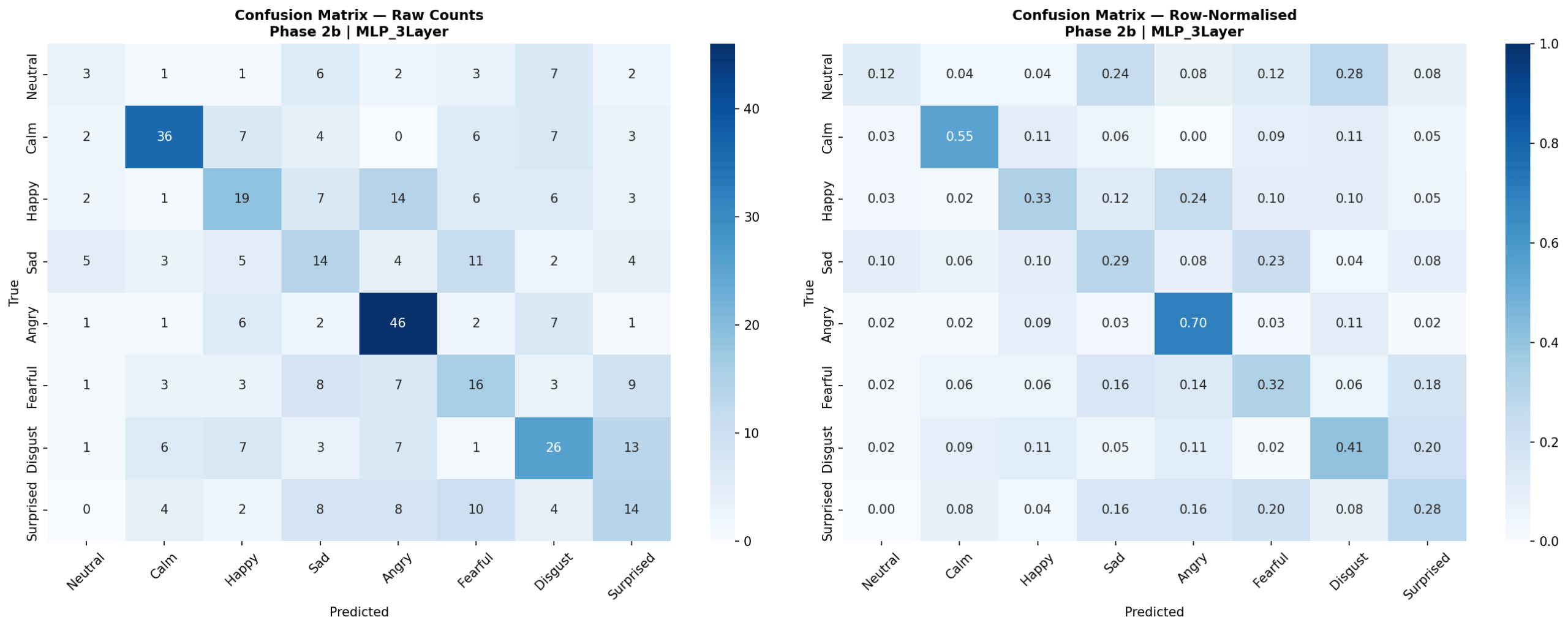
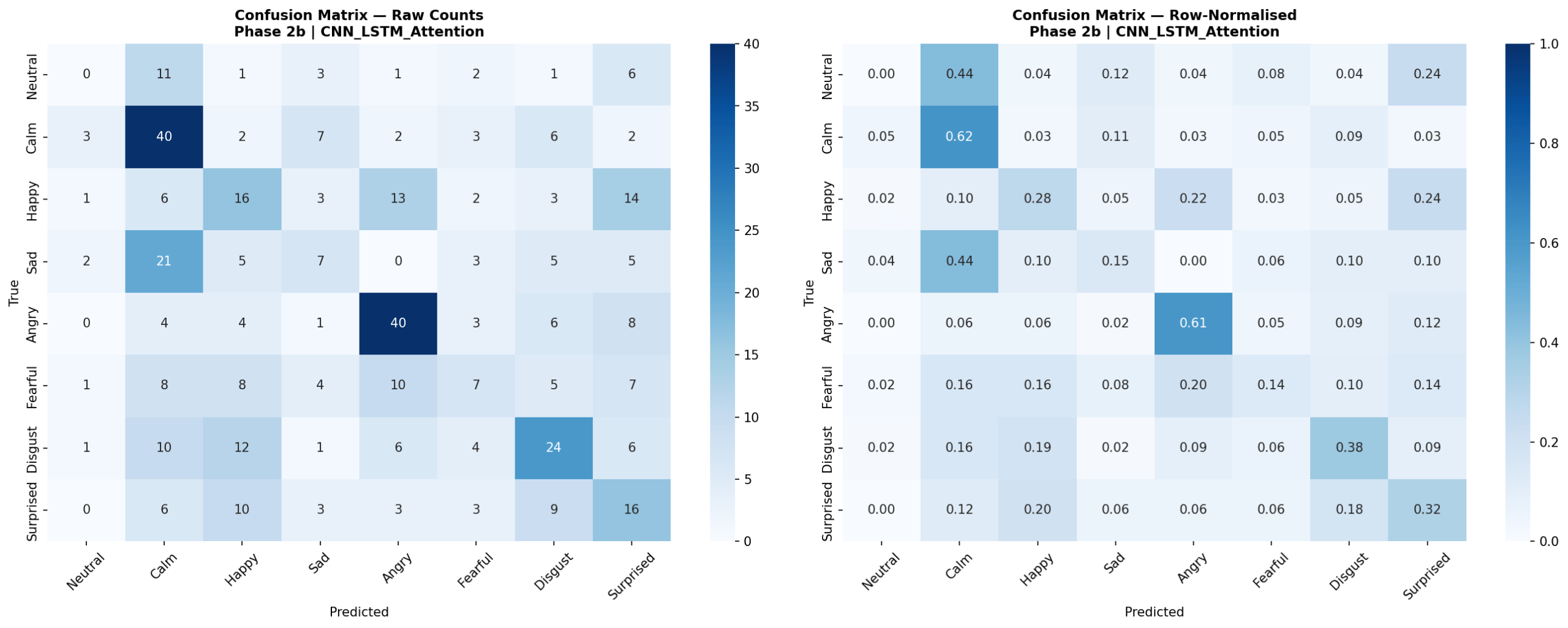
Figure 10 presents LOOCV results for all four neural models. MLP 3-Layer achieved the highest neural accuracy at 40.5% (SD = 7.2%, macro-F1 = 0.321, mean epochs = 39.8, 54,216 parameters, 10.5 s per fold). MLP 1-Layer reached 40.1% (SD = 11.6%, macro-F1 = 0.325, 6,920 parameters, 8.4 s per fold). 1D CNN achieved 40.1% (SD = 9.4%, macro-F1 = 0.320, 189,960 parameters, 7.7 s per fold). CNN-LSTM with Attention was the lowest-performing model overall at 34.7% (SD = 8.0%, macro-F1 = 0.254, 157,705 parameters, 17.0 s per fold). MLP 1-Layer showed the highest fold-to-fold variability (range: 21.9%-56.9%), while CNN-LSTM with Attention showed less variability but consistently lower accuracy. Confusion matrices for the best neural model (MLP 3-Layer) and CNN-LSTM with Attention are shown in Figures 11 and 12.

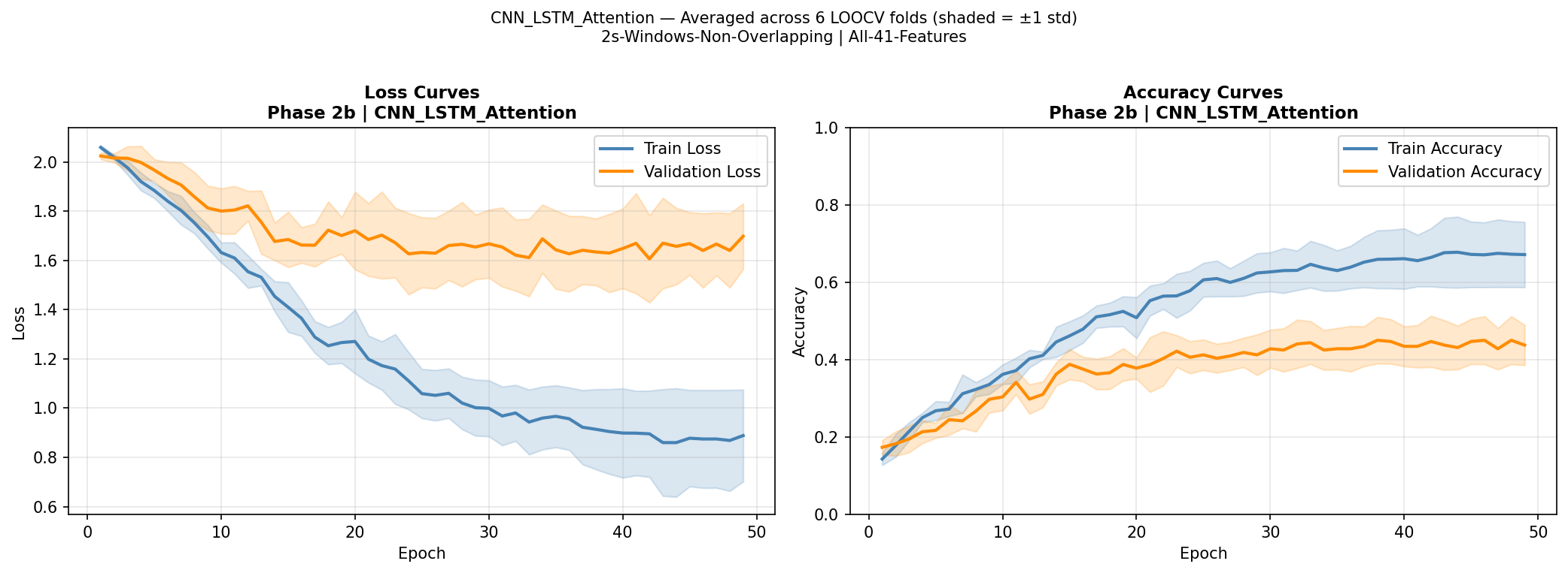
Training and validation curves averaged across all 6 LOOCV folds are shown in Figures 13-16. For MLP 1-Layer and MLP 3-Layer, training and validation accuracy tracked relatively closely before early stopping, with mean runs of 43.5 and 39.8 epochs respectively. The 1D CNN converged fastest (mean 23.2 epochs). CNN-LSTM with Attention showed a consistent pattern of training loss continuing to decrease while validation loss plateaued or increased after approximately 15-20 epochs, indicative  of overfitting.

Phase 3 – Focused Experiments

Test 4: Emotional Intensity

Figure 17 presents results for the four selected models evaluated separately on low-intensity (183 samples) and high-intensity (218 samples) subsets, using the 7-class dataset (Neutral excluded). Under high-intensity conditions, Logistic Regression achieved the highest accuracy at 55.1% (SD = 6.7%, macro-F1 = 0.471), followed by Random Forest at 53.7% (SD = 7.2%, macro-F1 = 0.466), MLP 3-Layer at 49.1% (SD = 8.8%, macro-F1 = 0.420), and CNN-LSTM with Attention at 45.5% (SD = 10.5%, macro-F1 = 0.379). Under low-intensity conditions, performance dropped substantially for all models: Random Forest 42.5% (SD = 13.9%, macro-F1 = 0.354), Logistic Regression 41.2% (SD = 9.2%, macro-F1 = 0.347), MLP 3-Layer 35.5% (SD = 6.9%, macro-F1 = 0.271), and CNN-LSTM with Attention 23.3% (SD = 8.4%, macro-F1 = 0.134). The accuracy gap between high and low-intensity conditions was approximately 11-13% for classical models and 14-22% for neural models. Confusion matrices for all four models under both intensity conditions are shown in Figures 18-25.

Test 5: Temporal Representation Confirmation

Figure 26 presents results for Random Forest and MLP 3-Layer evaluated across all three temporal conditions using the full 8-class dataset and all 41 features. For Random Forest, sentence-level features produced the highest accuracy at 43.9% (SD = 8.5%, macro-F1 = 0.385, n = 360), followed by 2-second windows at 41.8% (SD = 6.4%, macro-F1 = 0.336, n = 426), and 1-second windows at 33.8% (SD = 3.5%, macro-F1 = 0.294, n = 1,146). For MLP 3-Layer, 2-second windows produced the highest accuracy at 43.0% (SD = 9.1%, macro-F1 = 0.347, n = 426), followed by sentence-level at 38.9% (SD = 9.2%, macro-F1 = 0.331, n = 360), and 1-second windows at 30.9% (SD = 2.3%, macro-F1 = 0.279, n = 1,146). Both models showed a consistent and substantial drop at the 1-second window condition. Confusion matrices for all model-condition combinations are shown in Figures 27-32.

Discussion

Phase 1 – Representation Experiments

Interpretation of Feature Patterns

The feature importance results from Phase 1, Test 3 reveal that energy-based features were the primary acoustic drivers of emotion classification in this dataset, with Energy_std, Energy_max, and Energy_mean ranking first, second, and third respectively. This is acoustically interpretable: the RAVDESS emotion categories separate along the arousal (intensity) dimension more cleanly than along the valence (positive or negative emotion) dimension. High-arousal emotions such as Angry, Surprised, and Happy are produced with substantially elevated and dynamically variable vocal intensity, while low-arousal emotions such as Calm, Sad, and Neutral are produced with consistently lower and more stable energy levels. The dominance of Energy_std in particular reflects the importance of within-window energy variability, consistent with prior work identifying dynamic prosodic features as more discriminative than static averages⁶.

HNR ranked fourth in importance (4.46%), reflecting meaningful differences in vocal quality across emotion categories. Angry and Fearful speech are typically produced with increased laryngeal tension and aperiodic noise, yielding lower HNR values, whereas Calm and Neutral speech is produced with cleaner, more periodic phonation. Shimmer ranked ninth (3.20%), also consistent with its known sensitivity to emotional vocal perturbation. Together these voice quality features, while insufficient on their own (23.7% accuracy in isolation), provided complementary discriminative information that contributed to the 3.0 percentage point accuracy gain when combining all 41 features over MFCCs alone. This finding is consistent with work on the GeMAPS parameter set, which identifies perturbation measures as important secondary contributors to affective voice analysis⁶.

The most notable and unexpected finding in Phase 1 is that all five pitch-based features (Pitch_mean, Pitch_std, Pitch_min, Pitch_max, Pitch_range) received exactly zero importance from the Random Forest classifier, ranking 37th through 41st. Pitch is widely cited as a primary acoustic correlate of emotional arousal in the SER literature^6, making this result initially surprising. The most likely explanation is a methodological limitation of the pitch extraction pipeline: Librosa’s piptrack function extracts pitch candidates from spectrogram magnitude peaks across all frequency bins, and while only frames above the median magnitude and with a non-zero pitch value were retained, this filtering may not sufficiently isolate reliably voiced frames in all cases. In practice, many segments produced by piptrack may contain noisy or physiologically implausible pitch values, which when reduced to summary statistics (mean, std, range) yield features with low discriminative consistency across speakers and emotions. This interpretation is supported by the unusually flat distribution of pitch values across emotion categories in preliminary analysis. More robust pitch extraction approaches – such as RAPT or CREPE – would likely recover pitch as a meaningful feature, and represent an important direction for future work.

MFCCs were the strongest individual feature group at 37.3% accuracy (macro-F1 = 0.315), accounting for the majority of classification performance when used alone. The lower-order MFCCs (MFCC_1_mean, MFCC_5_mean) dominated the importance ranking among spectral features, reflecting their sensitivity to broad spectral shape differences – particularly the overall energy distribution and low-frequency resonance – that vary meaningfully across emotion categories. The prosody group achieved 32.8% accuracy when used alone, but this figure is reduced by the non-contribution of pitch; energy and ZCR features within the prosody group were doing the bulk of the work. The practical implication is that a compact 14-feature set (MFCCs + energy stats + ZCR, excluding pitch) would likely match the performance of the full 41-feature set at lower computational cost, though this was not formally tested in this study.

Impact of Temporal Resolution

The temporal segmentation experiment showed that sentence-level and 2-second non-overlapping windows produced equivalent performance with Logistic Regression (40.0% vs 40.9%), while 1-second windows caused a consistent decline to 31.0% – a drop of approximately nine percentage points. This threshold effect was confirmed in Phase 3, Test 5 using both Random Forest and MLP 3-Layer, where the 1-second condition produced the lowest accuracy in all cases. The consistency of this finding across three different models and two separate experimental phases provides strong converging evidence that 1 second represents an insufficient temporal context for the acoustic features used here.

At 1-second granularity, MFCC statistics are computed over very few short-time frames, reducing their statistical reliability. Energy summary statistics are particularly affected: a 1-second window may capture only a fraction of the prosodic arc of a word, and min/max/range statistics become increasingly sensitive to transient artifacts. ZCR statistics suffer similarly. The 2-second window appears to capture enough of the phonological and prosodic structure of a RAVDESS sentence – which ranges from 4 to 6 seconds total – to yield stable feature estimates. This is consistent with prior findings that emotional cues in speech are often encoded in short-term acoustic variations spanning several hundred milliseconds to a few seconds²³, and that reducing window size below a critical threshold can substantially degrade feature quality⁹.

Notably, for MLP 3-Layer in Phase 3 Test 5, the 2-second window condition slightly outperformed sentence-level (43.0% vs 38.9%), suggesting that neural models may benefit from the larger effective sample size that windowing provides – more training instances per fold – even when individual windows carry less contextual information. Random Forest showed the reverse pattern (43.9% sentence-level vs 41.8% for 2-second windows), suggesting that for classical models, richer per-sample features outweigh sample count advantages. This model-specific interaction between sample size and feature granularity is worth investigating further in future work.

Phase 2 – Model Comparison

Classical Model Performance

Random Forest achieved the highest classical LOOCV accuracy at 41.8% (macro-F1 = 0.336), marginally outperforming Logistic Regression at 40.3% (macro-F1 = 0.336). Both models substantially exceeded the 12.5% chance baseline – Random Forest by a factor of 3.3x – confirming that the 41 acoustic features carry meaningful emotion-discriminative information. SVC (37.8%) and Gradient Boosting (37.0%) performed modestly below the top two. All four models achieved macro-F1 scores of 0.30–0.34, indicating that performance, while above chance, was uneven across emotion classes rather than uniformly good.

The strong performance of Logistic Regression relative to its simplicity warrants discussion. As a parametric model (a model with a fixed number of learned coefficients) with a linear decision boundary, Logistic Regression makes stronger assumptions about the feature space than tree-based or kernel methods, but these assumptions become advantageous in low-data regimes: with approximately 300 training samples per fold and 41 features, there are insufficient data to reliably estimate the many non-linear interactions that Random Forest or Gradient Boosting can theoretically exploit. Logistic Regression’s L2 regularization further stabilizes its estimates by penalizing large coefficients. The practical implication is that the model’s constraint is a feature rather than a limitation in this context²⁴. SVC with a linear kernel performed below Logistic Regression (37.8%), likely due to its hinge-loss objective being less well-calibrated for the multi-class probability estimation task, while Gradient Boosting’s sequential tree-building process appears more susceptible to noise in small training sets despite its strong theoretical properties.

Confusion Matrix Analysis

Examining confusion matrices for the best classical models reveals consistent patterns of misclassification that align with the acoustic structure of the emotion space. Angry was the most accurately classified emotion across most models, consistent with its distinctive combination of high RMS energy, high energy variability, and elevated aperiodic voice quality (high jitter and shimmer, low HNR) – features that are acoustically distant from all other categories. Calm was also consistently well-classified, driven by its characteristically low and stable energy profile and high HNR, the opposite acoustic extreme from Angry.

The most frequent misclassification pairs were Sad and Calm, and Fearful and Surprised. Sad and Calm share low-arousal acoustic profiles – both are low-energy, low-intensity categories with relatively clean phonation – making them difficult to separate based on the features used here. Their primary distinction in naturalistic speech often involves subtle prosodic patterns (e.g., falling pitch contours in Sad) that were not reliably captured due to the pitch extraction limitation. Fearful and Surprised share high-arousal characteristics – elevated energy, wider pitch range, and increased voice perturbation – placing them in a similar region of feature space despite differing valences. Neutral was frequently misclassified as Calm, which is acoustically reasonable: both categories are produced with minimal affective emphasis and represent the low end of the arousal dimension in RAVDESS. These confusion patterns are consistent with the arousal-valence model of emotion, in which acoustically similar emotions occupying proximate regions of the affect space are harder to distinguish³

Model Complexity vs. Dataset Size

The central finding of Phase 2 is that increasing model complexity from classical to neural architectures provided no improvement in LOOCV accuracy. All three MLP and CNN configurations converged to approximately 40% accuracy – essentially matching the best classical models – while the CNN-LSTM with Attention underperformed at 34.7%. This pattern held despite substantial differences in parameter count: from 6,920 (MLP 1-Layer) to 189,960 (1D CNN), neither additional capacity nor more sophisticated sequential modeling translated into better generalization.

Training curves confirmed that overfitting was the primary reason for the CNN-LSTM’s underperformance. Training accuracy consistently reached higher levels than test accuracy across folds, and the divergence between training and validation loss was most pronounced for the CNN-LSTM, which also required the longest training time per fold (17.0 s vs 8.4 s for MLP 1-Layer) despite not benefiting from additional epochs. The attention mechanism, intended to focus the model on emotionally salient time steps within the pseudo-temporal feature sequence, did not provide the expected benefit – likely because the 41-feature vector processed by the CNN-LSTM does not represent a genuine temporal sequence, making the attention weights difficult to meaningfully learn from limited data²⁵. These results are consistent with a well-established principle in machine learning: deep architectures require large amounts of training data to learn generalizable representations, and with approximately 300 training samples per LOOCV fold, the representational capacity of CNNs and LSTMs confers no advantage over simpler parametric models²⁶. The MLP models, despite being neural networks, achieved competitive performance precisely because their architectures were constrained enough (6,920–54,216 parameters) to be trainable on small folds without severe overfitting. The finding that MLP 1-Layer matched MLP 3-Layer (40.1% vs 40.5%) further suggests that depth itself was not the limiting factor – the bottleneck was data volume.

It is important to contextualize the 40% peak accuracy appropriately. While substantially above the 12.5% chance baseline (a factor of 3.3x), it falls short of the 50–70% accuracy range reported in speaker-independent SER studies using larger or augmented datasets¹. This gap is expected given the constraints of this study: 6 actors, a small per-fold training set, and features that do not include pitch (a known arousal correlate) due to extraction limitations. The 40% figure should be understood as the approximate upper bound observed with this specific feature set and dataset size under strict speaker-independent evaluation, not as a measure of the ceiling for SER on RAVDESS generally. Under high-intensity conditions in Phase 3, Logistic Regression reached 55.1%, suggesting that with more acoustically distinct data the same models are capable of substantially higher performance.

Phase 3 – Focused Experiments

Influence of Emotional Intensity

The intensity analysis produced the most consistent and interpretable result in the study: all four models performed substantially better on high-intensity recordings than low-intensity recordings, with accuracy gaps of 11–14 percentage points for classical models and 14–22 percentage points for neural models. Logistic Regression achieved 55.1% on high-intensity recordings versus 41.2% on low-intensity, while CNN-LSTM with Attention showed the largest gap (45.5% vs 23.3%). This pattern is consistent with the acoustic properties of the RAVDESS intensity manipulation: high-intensity recordings are produced with more exaggerated affective signals – larger energy excursions, wider pitch ranges, more pronounced perturbation measures – that push emotion categories further apart in the feature space.

The CNN-LSTM’s disproportionately large intensity gap (22.2 percentage points) is particularly revealing. Under low-intensity conditions, the model’s tendency to overfit to training speaker characteristics left it with effectively near-chance performance (23.3%), suggesting it found no generalizable signal in the subtler acoustic markers of low-intensity emotional speech. Under high-intensity conditions, where affective signals are more pronounced and consistent across speakers, the model was able to extract some useful patterns, achieving 45.5%. This interaction between model complexity and signal strength reinforces the conclusion that complex architectures are poorly suited to this dataset size unless signal quality is high.

These findings have an important practical implication: the overall accuracy figures reported in Phase 2 represent a blend of high- and low-intensity performance. Systems designed specifically for high-intensity emotional speech – such as applications detecting distress, anger, or highly expressive communication – could achieve substantially higher accuracy with the same models and features. Conversely, detecting low-intensity or subtle emotional states remains a substantially harder problem, one that likely requires richer feature representations or substantially more training data.

Temporal Representation Confirmation

Phase 3, Test 5 confirmed the temporal segmentation findings from Phase 1 using the strongest classical model (Random Forest) and strongest neural model (MLP 3-Layer). Both models showed substantial degradation at 1-second windows (Random Forest: 43.9% sentence-level vs 33.8% at 1 second; MLP 3-Layer: 43.0% at 2-second windows vs 30.9% at 1 second), and broadly comparable performance between sentence-level and 2-second conditions. This convergence across three different models – Logistic Regression in Phase 1, Random Forest and MLP 3-Layer in Phase 3 – provides strong evidence that the 1-second threshold finding generalizes across model types, and that the selection of 2-second non-overlapping windows as the experimental standard was appropriate.

Broader Interpretation

Novelty and Contribution

By organizing experiments into three phases that progressively lock in optimal configurations before expanding model comparisons, and by enforcing consistent LOOCV evaluation across all experiments, this study provides a methodologically rigorous assessment of how feature choice, temporal granularity, and model complexity interact under strict speaker-independent conditions on a small, controlled dataset. The finding that pitch features contributed nothing due to extraction limitations, while energy and HNR dominated, is itself a practically useful result: it identifies a concrete methodological weakness (piptrack unreliability) and points toward specific improvements, rather than leaving feature importance ambiguous across a black-box model.

Limitations

Several limitations should be considered when interpreting these results. First, the experiments were conducted on 6 of the 12 available RAVDESS male actors, reducing the effective dataset size and the diversity of the speaker pool. This limits the generalizability of the findings to other speakers, even within the RAVDESS corpus, and means fold-level results carry higher variance than they would with a full 12-actor evaluation²⁷.

Second, RAVDESS is a laboratory-elicited, actor-performed dataset. Professional actors produce emotions with exaggerated acoustic markers designed for recognizability, which may not reflect the subtler and more variable emotional expressions found in naturalistic speech. Models trained on RAVDESS may therefore overestimate performance relative to what would be achieved on spontaneous conversational data¹⁰. Furthermore, all actors are North American English speakers, meaning results may not generalize to other languages or cultures where emotional prosody differs¹.

Third, the pitch extraction methodology was ineffective: all five pitch features received zero importance. This is a significant limitation given that pitch is one of the most theoretically important acoustic correlates of emotional arousal⁶. The failure of Librosa’s piptrack to produce discriminative pitch features likely suppressed overall model performance and prevented proper evaluation of prosodic features as typically defined in the literature. Future work should replace piptrack with a more robust pitch estimator.

Fourth, the male-only dataset limits generalizability to female speakers, who exhibit different baseline pitch ranges and potentially different emotional acoustic profiles. The use of a single dataset also means that cross-corpus generalization, a key challenge in practical SER deployment, was not evaluated.

Future Work

Several directions for future work follow directly from these findings. The most immediate is replacing Librosa’s piptrack with a robust pitch extractor such as CREPE or RAPT, which would allow proper evaluation of pitch features and likely improve overall accuracy. A second priority is expanding the dataset to the full 12-actor RAVDESS male subset and ideally including the female actors, which would double the fold size and reduce per-fold variance. Testing generalization to naturalistic datasets such as IEMOCAP or MSP-IMPROV would provide a more realistic estimate of deployed system performance. On the modeling side, testing transformer-based architectures or pre-trained speech representations such as wav2vec 2.0 fine-tuned for emotion recognition would be a natural next step for evaluating whether large-scale pretraining can overcome the small-dataset bottleneck identified here. Finally, a formal hierarchical model combining word-level and sentence-level features – motivated by the exploratory per-word pitch contour analysis – could test whether fine-grained temporal resolution provides classification benefit beyond what was demonstrated in the window-size experiments.

References

1. B. W. Schuller. Speech emotion recognition: Two decades in a nutshell, benchmarks, and ongoing trends. Communications of the ACM. Vol. 61, no. 5, pg. 90-99, 2018, https://doi.org/10.1145/3129340 [↩] [↩] [↩]
2. K. R. Scherer. What are emotions? And how can they be measured? Social Science Information. Vol. 44, pg. 695-729, 2005, https://doi.org/10.1177/0539018405058216. [↩]
3. J. A. Russell. A circumplex model of affect. Journal of Personality and Social Psychology. Vol. 39, pg. 1161-1178, 1980, https://doi.org/10.1037/h0077714 [↩] [↩]
4. P. Ekman. An argument for basic emotions. Cognition and Emotion. Vol. 6, no. 3-4, pg. 169-200, 1992, https://doi.org/10.1080/02699939208411068 [↩]
5. R. W. Picard. Affective Computing. MIT Press, Cambridge, MA, 1997, https://mitpress.mit.edu/9780262661157/affective-computing [↩]
6. F. Eyben, K. R. Scherer, B. W. Schuller, J. Sundberg, E. André, C. Busso, L. Y. Devillers, J. Epps, P. Laukka, S. S. Narayanan, K. P. Truong. The Geneva minimalistic acoustic parameter set (GeMAPS) for voice research and affective computing. IEEE Transactions on Affective Computing. Vol. 7, no. 2, pg. 190-202, 2016, https://doi.org/10.1109/TAFFC.2015.2457417 [↩] [↩] [↩] [↩] [↩] [↩]
7. Z. Zhao, D. Xu, S. Zhang, Z. Zou, L. Zhang, E. Song. Speaker-invariant affective representation learning via adversarial training. arXiv preprint. arXiv:1911.01533, 2019, https://ar5iv.labs.arxiv.org/html/1911.01533 [↩]
8. Y. Zhang, J. Du, Z. Wang, J. Zhang. Attention based fully convolutional network for speech emotion recognition. 2018 Asia-Pacific Signal and Information Processing Association Annual Summit and Conference (APSIPA ASC). pg. 1771-1775, 2018, https://doi.org/10.23919/APSIPA.2018.8659587 [↩]
9. B. Schuller, S. Steidl, A. Batliner, F. Burkhardt, L. Devillers, C. Müller, S. Narayanan. The INTERSPEECH 2009 Emotion Challenge. Proceedings of INTERSPEECH 2009. 2009, https://www.researchgate.net/publication/224929671_The_Interspeech_2009_Emotion_Challenge [↩] [↩]
10. S. R. Livingstone, F. A. Russo. The Ryerson audio-visual database of emotional speech and song (RAVDESS): A dynamic, multimodal set of facial and vocal expressions in North American English. PLOS ONE. Vol. 13, no. 5, p. e0196391, 2018, https://doi.org/10.1371/journal.pone.0196391 [↩] [↩]
11. B. McFee, C. Raffel, D. Liang, D. P. Ellis, M. McVicar, E. Battenberg, O. Nieto. Librosa: Audio and music signal analysis in Python. Proceedings of the Python in Science Conference. Austin, Texas, 2015, pg. 18-24, https://doi.org/10.25080/Majora-7b98e3ed-003 [↩]
12. Torchaudio Team. Forced alignment with Wav2Vec2. PyTorch Documentation. 2025. https://docs.pytorch.org/audio/stable/tutorials/forced_alignment_tutorial.html [↩]
13. S. B. Davis, P. Mermelstein. Comparison of parametric representations for monosyllabic word recognition in continuously spoken sentences. IEEE Transactions on Acoustics, Speech, and Signal Processing. Vol. 28, no. 4, pg. 357–366, 1980, https://doi.org/10.1109/TASSP.1980.1163420 [↩]
14. K. R. Scherer. Vocal affect expression: A review and a model for future research. Psychological Bulletin. Vol. 99, no. 2, pg. 143–165, 1986, https://doi.org/10.1037/0033-2909.99.2.143 [↩]
15. C. Cortes, V. Vapnik. Support-vector networks. Machine Learning. Vol. 20, no. 3, pg. 273–297, 1995, https://doi.org/10.1007/BF00994018 [↩]
16. Scikit-learn Developers. RandomForestClassifier. Scikit-learn Documentation. 2025, https://scikit-learn/stable/modules/generated/sklearn.ensemble.RandomForestClassifier.html [↩]
17. L. Breiman. Random forests. Machine Learning. Vol. 45, no. 1, pg. 5–32, 2001, https://doi.org/10.1023/A:1010933404324 [↩]
18. N. Srivastava, G. Hinton, A. Krizhevsky, I. Sutskever, R. Salakhutdinov. Dropout: A simple way to prevent neural networks from overfitting. Journal of Machine Learning Research. Vol. 15, no. 1, pg. 1929–1958, 2014, https://dl.acm.org/doi/10.5555/2627435.2670313 [↩]
19. S. Hochreiter, J. Schmidhuber. Long short-term memory. Neural Computation. Vol. 9, no. 8, pg. 1735–1780, 1997, https://doi.org/10.1162/neco.1997.9.8.1735 [↩]
20. Y. LeCun, Y. Bengio, G. Hinton. Deep learning. Nature. Vol. 521, pg. 436–444, 2015, https://doi.org/10.1038/nature14539 [↩]
21. D. P. Kingma, J. Ba. Adam: A method for stochastic optimization. arXiv preprint. arXiv:1412.6980, 2015, https://arxiv.org/abs/1412.6980 [↩]
22. A. Batliner, S. Steidl, C. Hacker, E. Nöth. Speaker normalisation for speech-based emotion detection. Proceedings of the International Conference on Speech and Language Processing. 2009, https://www.researchgate.net/publication/224719010_Speaker_Normalisation_for_Speech-Based_Emotion_Detection [↩]
23. M. Grimm, K. Kroschel, E. Mower, S. Narayanan. FEELTRACE: An instrument for recording perceived emotion in real time. Proceedings of the IEEE International Conference on Acoustics, Speech and Signal Processing (ICASSP). 2007, https://www.researchgate.net/publication/209436026_FEELTRACE_An_instrument
    _for_recording_perceived_emotion_in_real_time [↩]
24. J. de Lope, M. Graña. An ongoing review of speech emotion recognition. Neurocomputing. Vol. 528, pg. 1-11, 2023, https://doi.org/10.1016/j.neucom.2023.01.002 [↩]
25. S. Tripathi, S. Tripathi, A. Beigi. Speech emotion recognition using deep 1D and 2D CNN LSTM networks. Biomedical Signal Processing and Control. Vol. 47, pg. 312-323, 2019, https://doi.org/10.1016/j.bspc.2018.08.035 [↩]
26. T. Latif, R. Rana, R. Jurdak. Adversarial machine learning and speech emotion recognition: Utilizing generative adversarial networks for robustness. arXiv preprint. arXiv:1812.01810, 2018, https://www.researchgate.netpublication/329266548_
    Adversarial_Machine_Learning_And_Speech_Emotion_Recognition_Utilizing_Generative_
    Adversarial_Networks_For_Robustness [↩]
27. B. Schuller, G. Rigoll, M. Lang. Hidden Markov model-based speech emotion recognition. Proceedings of the IEEE International Conference on Acoustics, Speech and Signal Processing (ICASSP). Vol. 2, pg. II–1–II–4, 2003, https://doi.org/10.1109/ICASSP.2003.1202279 [↩]