
Abstract
I investigate strategies for semantic decoding from minimal-channel, consumer-grade EEG systems. Using only four electrodes and 50–100 word stimuli, I evaluate convolutional architectures on two semantic tasks including emotional valence and part-of-speech discrimination (specifically, noun/verb classification). First, to address limited data, I introduce a data amplification method based on short-time FFT snapshots. Secondly, I introduce an embedding-constrained EEG architecture that leverages clustered word embeddings to design specialized processing branches without requiring embeddings at inference. Spectral (FFT) data improved accuracy by ~8% over time-series models, while the embedding-constrained architecture reached ~93.6% ± 1.4, outperforming baselines and multi-head models.
Keywords: EEG, FFT, EEGNet, word embeddings, embedding-constrained architecture, brain–computer interface, semantic decoding
Introduction
Decoding semantic information from non-invasive electroencephalography (EEG) is a sought after goal, especially for NLP applications, with applications for brain–computer interfaces (BCIs), cognitive neuroscience, and areas of neurotechnology1. Recent convolutional neural network approaches (e.g., EEGNet-style architectures) have demonstrated the ability to classify mental states and categories from relatively small EEG datasets by encoding biases into compact models2. Other work has demonstrated that semantic categories and individual word meanings can be inferred from brain activity patterns and signals3,4. More recent advances in deep learning have extended these ideas to EEG decoding, most of which leverage neural networks and embeddings to map neural signals to certain semantic representations5,6. However, these approaches typically depend on high-density EEG recordings (i.e. many channels) and large datasets, all of which limit the practicality of these models.
Nowadays, many decoders, while effective in controlled laboratory environments, are incredibly data-intensive and fail under low-channel and minimal-trial conditions (here, signal-to-noise ratios (SNRs) are reduced)7,8,9. Prior work has also shown that reducing electrode count introduces tradeoffs and decreases decoding reliability and especially generalization, all which hinders semantic decoding performance10. Additionally, it’s important to point out that many existing methods don’t build language structure directly into their architecture. Instead, they try to learn this structure from data or embeddings, which causes poor performance when data is limited11. At the same time, frequency-domain representations (known to be very informative for EEG analysis) remain underutilized as a means of amplifying sample size for semantic decoding tasks9. This leaves a gap in current EEG decoding research: there is an absence of architectures that leverage linguistic structure during model design while remaining independent of inference, particularly under minimal channel and limited data constraints8.
In this experiment, I am faced with exactly these constraints. First, consumer EEG devices (here, OpenBCI Ganglion and the corresponding headband) provide only a handful of channels. It is true that developing reliable decoders from minimal-channel recordings is essential for low-cost, real world systems12. Second, many uses require strong performance from very limited data (tens of stimulus presentations) so methods that utilize information content without collecting more raw trials are valuable. To be transparent, the following experiment aims to serve as a proof-of-concept investigation with this goal in mind, rather than a demonstration of a general, real-world, semantic decoding system. This experiment is focused on generating high-accuracies for within-subject, specific tasks, and not intended to serve as a generalizable system.
I investigate two strategies to address these constraints and prevailing issues. The first is a frequency-domain data amplification approach: by capturing FFT representations and sampling many FFT “plots” per trial, one can obtain many more training samples from few trials while preserving key signatures (see Appendix B: Flowchart 2). Here, data amplification is different from data augmentation; data amplification is the careful enlarging of a dataset and extracting more information from minimal samples. The second is a linguistically informed architectural approach. Rather than feeding word embeddings into the model at inference (which can cause overfitting and dependence), I use embeddings only during architecture design. I call this the Embedding-Constrained EEG Architecture.
In addition to these two strategies, I also evaluated some standard baselines: time-series trained EEGNet-style models, LIME and weight-based explainability to inform channel reweighting, a fused multi-head model constructed from existing, single-task models, and an alternative regularizer strategy that attempts to force EEG features toward embedding predictions. I compare performance on two semantic decoding tasks commonly used in EEG studies: emotional valence classification (negative / neutral / positive) and part-of-speech (POS) discrimination (in this case, noun vs. verb)13. Importantly, I evaluate under the strict constraints discussed previously: four channels and as few as 50 trials per person.
I hypothesized that FFT-based sampling will substantially improve classifier performance relative to raw time-series data by carefully increasing effective sample size and making spectral features clear. Additionally, I hypothesized that the embedding-constrained architectural design will outperform embedding-as-regularizer approaches and even single-task baseline EEGNet-style models by incorporating relevant inductive biases. Finally, I hypothesized that while channel reweighting will further boost single-participant accuracy by reducing general artifactual influence, leveraging embeddings will allow for a simpler, less tedious path to similar accuracies.
Methods
Participants
For the participant-related details in this study, results for single-participant and participant-level analyses are reported on a per-subject basis. Similar to approaches taken by Sun et al. and Wandelt et al., the analysis involved a small number of participants (n=2), which puts the emphasis on single-participant decoding rather than large-scale group-level, generalizable efforts14,15. Most models were trained independently on each participant’s dataset, with evaluation metrics averaged across the two. Cross-participant evaluations have not yet been conducted, and as a result, remains an important direction for future research. From a practical perspective, these models are designed to be readily trained, adapted and fine tuned to individual participants, and even across tasks, with relative ease.
Hardware & Acquisition
The hardware and data acquisition setup utilized the OpenBCI Ganglion board paired with OpenBCI flat and comb-style electrodes. Four active channels were used and positioning was configured for semantic decoding purposes (schematic shown in Figure 1). In both experimental tasks, electrodes were positioned at TP7, TP8, F7, and F8 according to the international 10-20 system (see Figure 1)12. Data was streamed in real time from the OpenBCI GUI using the built in Lab Streaming Layer (LSL) for real time data acquisition.
The EEG data was sampled at a rate of 200 Hz, segmented into 5-second epochs containing 1000 time points per sample. For each trial, both raw time-series data and FFT data were collected; FFT data was taken in 250 temporal snapshots across the 5-second sampling period.
Impedance and signal quality were monitored by checking all channels prior to the start of each recording session through a visual cue on the OpenBCI GUI (red signaled high impedance, yellow signaled low impedance etc.) No trials were omitted as none exhibited a red signal. Signals with an impedance signal of yellow (slight impedance) were included.
Stimuli & Experimental Design
Stimulus presentation involved displaying individual words on a monitor, with a fixation cross presented between trials to reduce eye-movement artifacts. Each word (stimulus) was shown for a fixed duration of 5 seconds, followed by a “relaxation” interval of approximately 1–2 seconds. To clarify, each participant underwent 2 sessions in which they were shown 50 unique words (stimuli). Each word I will refer to as a “trial”. See the table below for an overview of the experimental design.
| Parameter | Count | Definition |
|---|---|---|
| Sessions | 2 | Single recording session per participant per task (1 for emotional valence, another for noun/verb) |
| Total Unique Words | 100 | No word repetitions across entire experiment |
| Repetitions Per Word | 0 | Each word presented exactly once |
| Words Per Class | 50 | 50 words for emotional valence / 50 words for noun/verb |
| Trials Per Class | 50 | One trial = one word presentation |
| Total Trials Per Participant | 100 | 50 (Class A) + 50 (Class B) |
| Snapshots Per Trial | 125 | 125 FFT snapshots per word/trial |
| Total Snapshots Per Participant | 12500 | (100 words in total across both classes) × 125 snapshots per word |
The experimental design included two primary semantic classification tasks. The first was an emotional valence task, in which words were categorized as negative, neutral, or positive, and the second was a part-of-speech task (i.e distinguishing nouns from verbs). Each task utilized a set of 50 unique words, as described in the introduction. Words were presented once per participant (zero repetitions), and participants were instructed to actively ponder the meaning and implication of each word while viewing it, rather than merely passively observing.
To increase the effective training sample size for the FFT-based decoding approach, data amplification was applied during feature extraction: within each 5-second epoch, every other FFT “window” or temporal snapshot was treated as an independent training sample (see Feature Extraction section for details). This resulted in 125 usable FFT samples per 5-second word presentation (after skipping every other snapshot). Consequently, a single task with 50 words yielded 50 × 125 = 6,250 FFT samples per participant, while combining both tasks (100 unique words total) produced 12,500 FFT samples available for model training and evaluation.
EEG Preprocessing
EEG preprocessing was conducted entirely through a custom pipeline developed using NumPy, TensorFlow, and Scikit-learn. It’s important to note that bandpass filtering and line-noise removal occurred automatically during real-time data streaming. The “timeseriesfilt” stream capability from the OpenBCI LSL software applies these filters automatically, eliminating the need for any additional offline bandpass or notch processing.
The preprocessing sequence consisted of the following steps. First, bandpass filtering was applied over the 0.5–100 Hz range (handled automatically within the filtered LSL stream). Second, line-noise removal was achieved via notch filtering at both 50 Hz and 60 Hz to eliminate electronic interference (again performed automatically by the “timeseriesfilt” stream). Third, normalization was carried out using a percentile-based method applied to each channel. For every channel, signal values were rescaled according to the range spanning the 5th to 95th percentiles. This normalization technique mitigates the influence of extreme outliers and artifacts (very important in the case of EEG), promotes greater consistency across recording sessions and participants, and was executed as the final step immediately before the data were inputted into the decoding models. This method was chosen over log-scaling or z-scoring as it makes no assumptions about the underlying data distribution and is better suited for the “messiness” and abnormalities of neural signals.
Feature Extraction & FFT Sampling
With regards to sampling, I compared two methods of sampling and representation.
The first approach used raw time-series data. After preprocessing, each 5-second epoch retained its original shape of (channels, timepoints) and was fed directly into the convolutional neural network. For compatibility with the EEGNet-inspired baseline model, an additional dimension was appended, resulting in an input shape of (channels, timepoints, 1).
The second approach employed an FFT-based representation and sampling method, which utilized a form of data amplification (illustrated in Appendix B: Flowchart 2). The motivation for this method stemmed from not only the ability of frequency-domain features to highlight activity in certain bands (e.g delta, theta, alpha, beta, gamma) but also given the known fact that more data improves models. Within each trial, the sliding FFT produced approximately 250 temporal “snapshots” over the 5-second trial duration. To increase the dataset size while maintaining integrity, I implemented two strategies inspired by Lashgari et al., 202016. First, all train/validation/test splits were performed at the trial level, ensuring no snapshots from the same trial appeared across different dataset groups. Second, within each trial, we sampled every other snapshot (yielding 125 samples per trial) rather than using all consecutive snapshots, as this would yield high temporal dependency. Note that taking FFT snapshots at a reduced frequency (every 10th snapshot instead of every 2nd) scales is indirectly proportional to accuracy. In other words, less FFT data correlated with lower accuracies. Also, it’s critical to point out that the FFT implementation used non-overlapping windows (window size = ~ 20 ms), ensuring that each snapshot was computed from entirely distinct segments of the raw signal as inspired by Huang et al., 202317. The sampled snapshots therefore represent disconnected 20 ms epochs with a 40 ms gap between consecutive samples, eliminating any direct signal overlap between training samples while reducing short-range correlation in samples themselves. The validity of this approach is supported by our results: models trained on subsampled FFT snapshots outperformed those using averaged representations (49.5% accuracy), demonstrating that the temporal structure captured by individual snapshots contains genuine discriminative information rather than leakage artifacts. Furthermore, LIME analysis revealed these “FFT amplified” models learned to prioritize artifact-free channels and suppress noise-contaminated channels (Figure 6) without intervention, indicating the model discovered valid patterns rather than exploiting dependencies. While we acknowledge that complete statistical independence between snapshots cannot be guaranteed due to the inherent structure and unknown patterns of neural signals, the approach balances the practical need for adequate sample size with a concious mitigation of “residual dependency”, especially in the case of single-participant, low-data, , task-specific, within-session decoding16.
The FFT extraction used the following parameters. Frequency content was limited to 1–60 Hz, producing 60 bins per snapshot. After sampling every other “frame”, 125 snapshots per trial were retained. Each individual FFT snapshot underwent the same percentile-based normalization (5th–95th range per channel) as applied to the time-series data. For input to convolutional networks, every snapshot was reshaped into a 2D representation of (channels, frequency bins), or (4, 60). The resulting snapshot input remained three-dimensional (consistent with the time-series format).
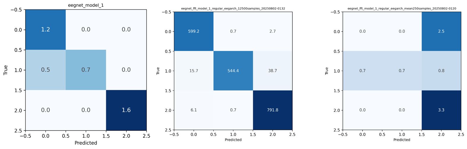
When processing 50 word trials via FFT, the raw collected shape was a four-dimensional shape of (50 trials, 250 snapshots, 4 channels, 60 bins). After selecting every other snapshot, this expanded to approximately (6250 samples, 4 channels, 60 bins), making the data directly compatible with standard CNN batch processing (with a 3 dim input shape). Alternative strategies were also examined, including averaging across all 250 snapshots per trial to produce a compact shape of (50, 4, 60); however, as anticipated, this was “lossy” and led to notably poorer decoding performance compared with the amplified dataset (see Appendix B: Confusion Matrix 1 for quantitative comparison).
Model Architectures & Development Pipeline (see Appendix A for detailed architectures)
I developed the modeling strategy iteratively. Starting from an EEGNet-style baseline trained on time series data, I moved to spectral inputs (FFT snapshots) to amplify effective sample size and expose frequency features. Explainability via LIME and early-layer weight evaluations then guided multiplicative channel reweighting (which reduced artifacts/noise). To efficiently reuse trained models across tasks I built a fused multi-head model that concatenates early weights and uses task-specific heads. Finally, leveraging word-embedding clusters to add biases, I designed the Embedding-Constrained architecture consisting of cluster-specific branches (e.g. emotion-focused low-frequency branch; sensory-focused high-frequency branch). An alternative strategy that enforced embedding prediction as an “auxiliary regularizer” was evaluated but found to show unstable optimization, over dependencies, and poor accuracies18. Hence, I focus on the embedding-constrained approach as the primary model. Below is a more detailed description of each of these approaches.
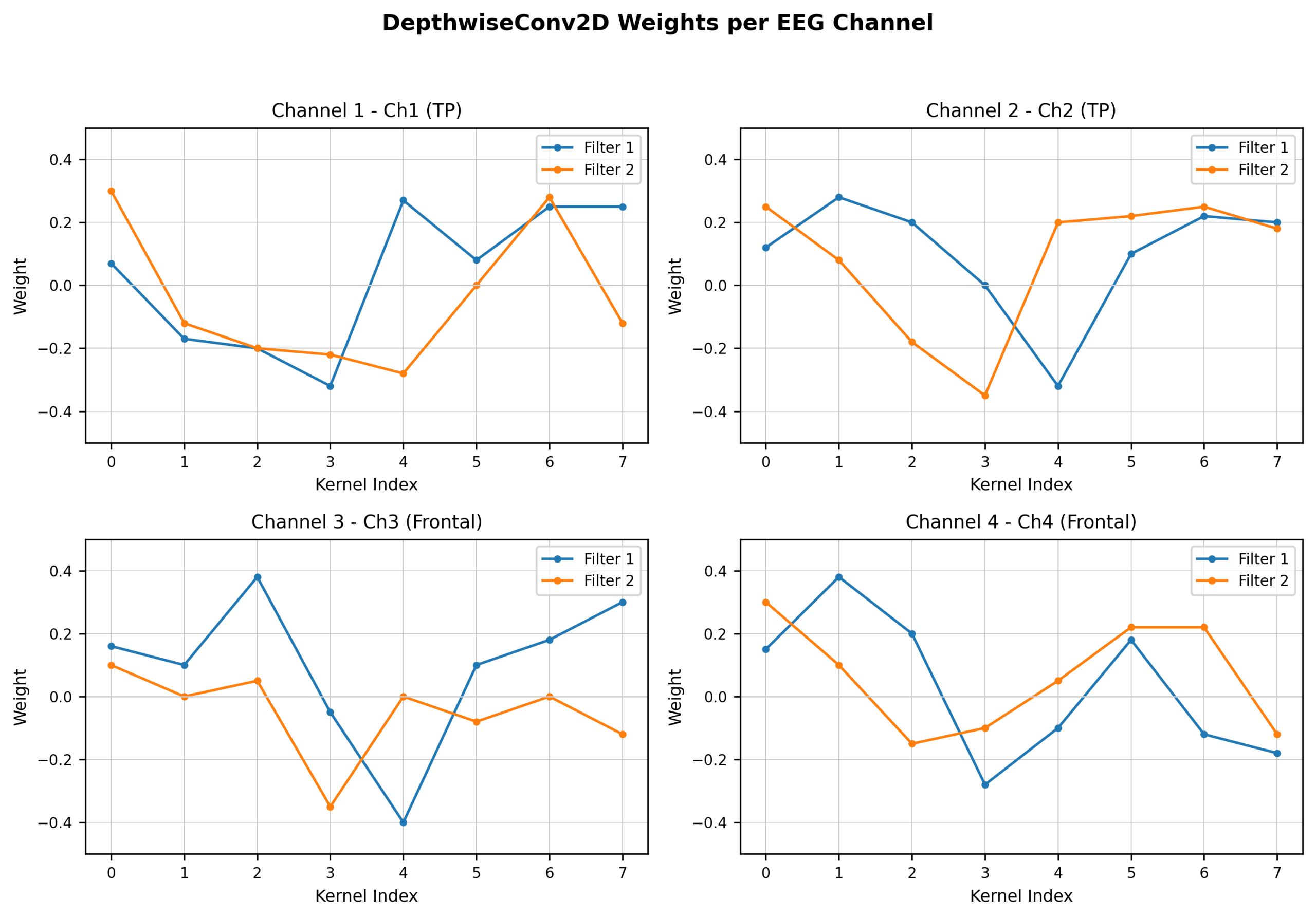
First, an EEGNet-style baseline was implemented following the compact convolutional architecture originally proposed in EEGNet, which employs multiple specialized filters to efficiently capture “spatiotemporal patterns” in EEG signals with a relatively small model2. The main layers included depthwise (for spatial filtering) followed by separable convolutions (capture temporal dynamics).
Several variants were explored to enhance interpretability and performance. First, LIME-guided channel reweighting was incorporated. After training the EEGNet-style models, early-layer weights were extracted and LIME (Local Interpretable Model-agnostic Explanations) was applied to measure the contribution of each channel to the predictions/outputs, while also helping to identify channels infected by artifacts or noise. Channels were then reweighted (multiplicative scalar) at the input level according to their estimated importance (essentially down-weighting noisy or uninformative channels and boosting those that were informative).
Second, a fused multi-head model was developed through fusion. Separate single-task models were first trained independently for the emotional valence and part-of-speech tasks. Their early convolutional weights were then extracted, concatenated to form a shared “fused” encoder, and task-specific classification heads were attached. It’s worth noting that an attention mechanism was introduced early on to enable the model to prioritize certain features during certain tasks. In the end, the features are concatenated, however. This process demonstrated the feasibility of multi-task fusion but ultimately highlighted the diminishing performance of smaller, multi-task systems.
The primary proposed model, named the Embedding-Constrained EEG Architecture, introduced a neuroscience informed design (detailed model specifications are provided in the Results section, Figure F, and Appendix A: Tables A1, A2, A3). The pipeline proceeded as follows. Word embeddings for the complete stimulus set (n = 100 words) were first generated using OpenAI’s text-embedding-3-small model (dim = 1536)19. These embeddings were then clustered into K semantic archetypes (K was arbitrarily selected to demonstrate a proof of concept; in the reported experiments K = 2), yielding clusters that captured broad semantic groupings such as emotional valence, concrete/sensory content, abstract concepts, noun-like versus verb-like properties, and other distinctions. Increasing K would improve robustness of the model and increase the nuance of these groups; however, it would also increase complexity. Cluster identities were determined by inspecting the words nearest to each centroid, which served as representative examples for interpreting and labeling that archetype/cluster.
For each identified grouping, a dedicated processing branch was constructed, with convolutional filter sizes biased toward frequency bands known to carry relevant neural signatures for that group (e.g., emphasizing delta, theta, and alpha bands for emotion-related processing; incorporating beta and gamma bands for noun/verb distinctions)20,13. This was informed by current literature which finds that “delta, alpha, and beta frequency bands correlate highly with emotions” and “theta power increases for verbs as compared to nouns”21,22. Each branch received FFT-based input in the form of (channels, frequency bins). Branch outputs were concatenated and fed into shared dense layers before branching again into task-specific classification heads. It’s important to note that word embeddings were used exclusively during architecture construction and never provided as input during training or inference. This ensured the model was forced to discover genuine EEG patterns rather than shortcutting to the cleaner semantic information from the embeddings (earlier tests showed that including embeddings directly in training frequently caused the model to over-rely on them and hinder the learning of EEG representations).
As an alternative strategy for comparison, an embedding-as-regularizer approach was also implemented. This alternative approach introduced an auxiliary loss term that encouraged the learned EEG feature embeddings to align with the corresponding word embeddings via cosine similarity. The intention was to bring about a shared embedding space that represented neural signals and text meaning. However, this regularization strategy led to over dependence on the embedding signal, and ultimately poorer decoding performance compared to the embedding-constrained architecture. Despite this, it was included here to explore different ways of leveraging pretrained word embeddings (which are rich in information) in EEG decoding.
Loss Functions & Optimization
Loss functions used categorical cross-entropy combined with focal loss (gamma = 1.5, alpha = 0.25). This choice addressed the ever-so-slight class imbalance present in the emotional valence task (20 positive, 15 neutral, 15 negative words), while the part-of-speech task remained naturally balanced.
The Adam optimizer was used consistently, with an initial learning rate of 1e−3 when training models from scratch and 1e−4 when training fused models. Batch sizes were set to 32 for the FFT-snapshot inputs to leverage the larger effective sample size, while smaller batches of 16 were used for raw time-series inputs with memory constraints in mind.
Training ran for a maximum of 100 epochs, with early stopping triggered after 20 epochs of no improvement in validation loss.
Evaluation Metrics & Statistical Tests
Evaluation metrics and statistical tests centered on classification accuracy as the primary performance measure. Chance-level baselines were 33.3% for the three-class emotional valence task and 50% for the binary part-of-speech task. Other analyses included confusion matrices, LIME-based interpretability outputs, and visualizations of learned convolutional weights.
To get accuracy estimates, the following procedure was applied after final training: the validation or test set was repeatedly shuffled, a random subset comprising 40–80% of the samples was drawn without replacement, the model was evaluated on that subset, and this process was repeated 100 times. The resulting accuracies were averaged to mitigate the influence of any particular data ordering or bias. Final reported accuracies are coupled with 95% Wilson confidence intervals. Cross validation was not utilized due to the use of non-overlapping snapshots. Cross validation would mix these snapshots and cause data leakage. By controlling the held-out test set we can work to mitigate this issue while still amplifying data for the model.
Also, the following is important to note: while accuracy is reported at the snapshot level, trial-level majority vote accuracy can be estimated analytically. Given 125 snapshots per trial at even 90% snapshot accuracy, the probability of majority vote misclassifying a trial is negligibly small, suggesting trial-level accuracy would not meaningfully shift in any way.
Explainability & Reweighting
Furthermore, LIME was applied to the trained EEGNet-style models to estimate per-channel contributions to sample predictions. These LIME scores directly informed channel reweighting. Again, in other words, channels consistently flagged as artifact-heavy or “not very” predictive were assigned a multiplicative down-weighting scalar at the input stage, after which the affected models were trained again. Performance with and without this reweighting step is reported, along with experiments that involved no reweighting.
Results
To determine whether FFT data improves classifier performance relative to raw time-series input, I trained identical EEGNet-style architectures on preprocessed time-domain epochs and FFT snapshots derived from the exact same trials (data amplification was conducted for FFT samples as discussed in Methods). Both models are single-task models without custom layers or adaptations.
It was concluded that FFT-trained models significantly outperformed time-series models for both emotion and POS tasks, indicating that FFT data both exposes valuable features and allows for increasing training sample size, which in turn, is shown to benefit model performance (see Figure 1). Specifically, FFT models outperformed time-series by ~8% on emotion and ~4% on POS (Figure. 2; see Appendix B: CM 2 for POS). All the models in Figure 1 consisted of the original architecture outlined in Appendix A: Table B1.
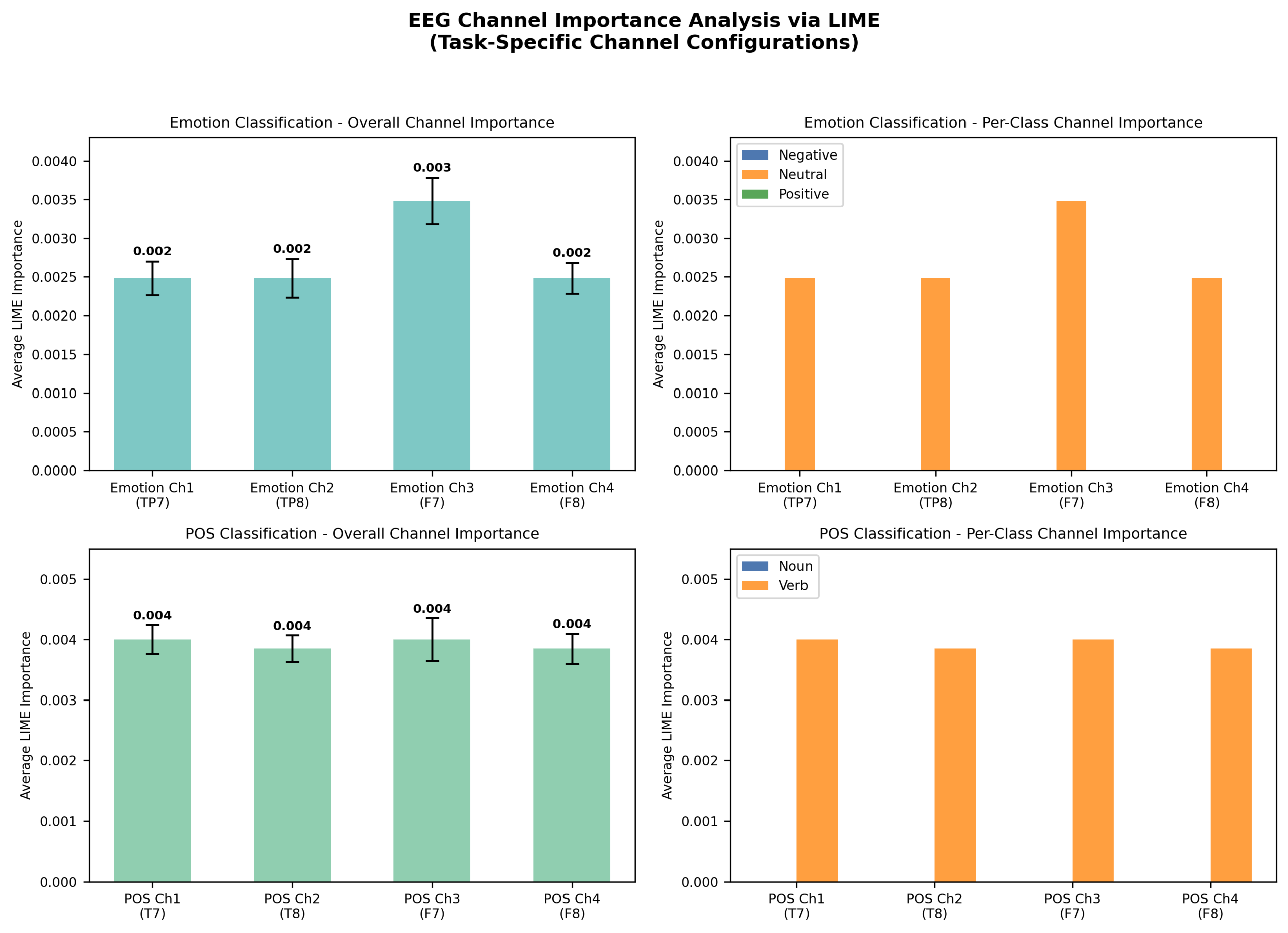
To identify channel/frequency contributions and reduce artifactual/noise influence in the baseline time-series model, I applied LIME and early-layer weight visualization, and tested multiplicative channel reweighting followed by re-training on the baseline time-series model evaluated in Figure 1. LIME indicated that channels 1 and 2 contributed most to emotion discrimination, and were therefore not modified with weights. After weight visualization, Channels 3 showed artifact-like signatures (e.g. spikes including EMG likely from eye movements hence the symmetric oscillations) and were then used for down-weighting (see Figure 2). Figure 3 graphs the influence of individual channels from the LIME analysis. I applied multipliers w (0 < w ≤ 1) to channels with artifacts or heavy negative influence (channels 3 and 4) then retrained the model (see Methods).
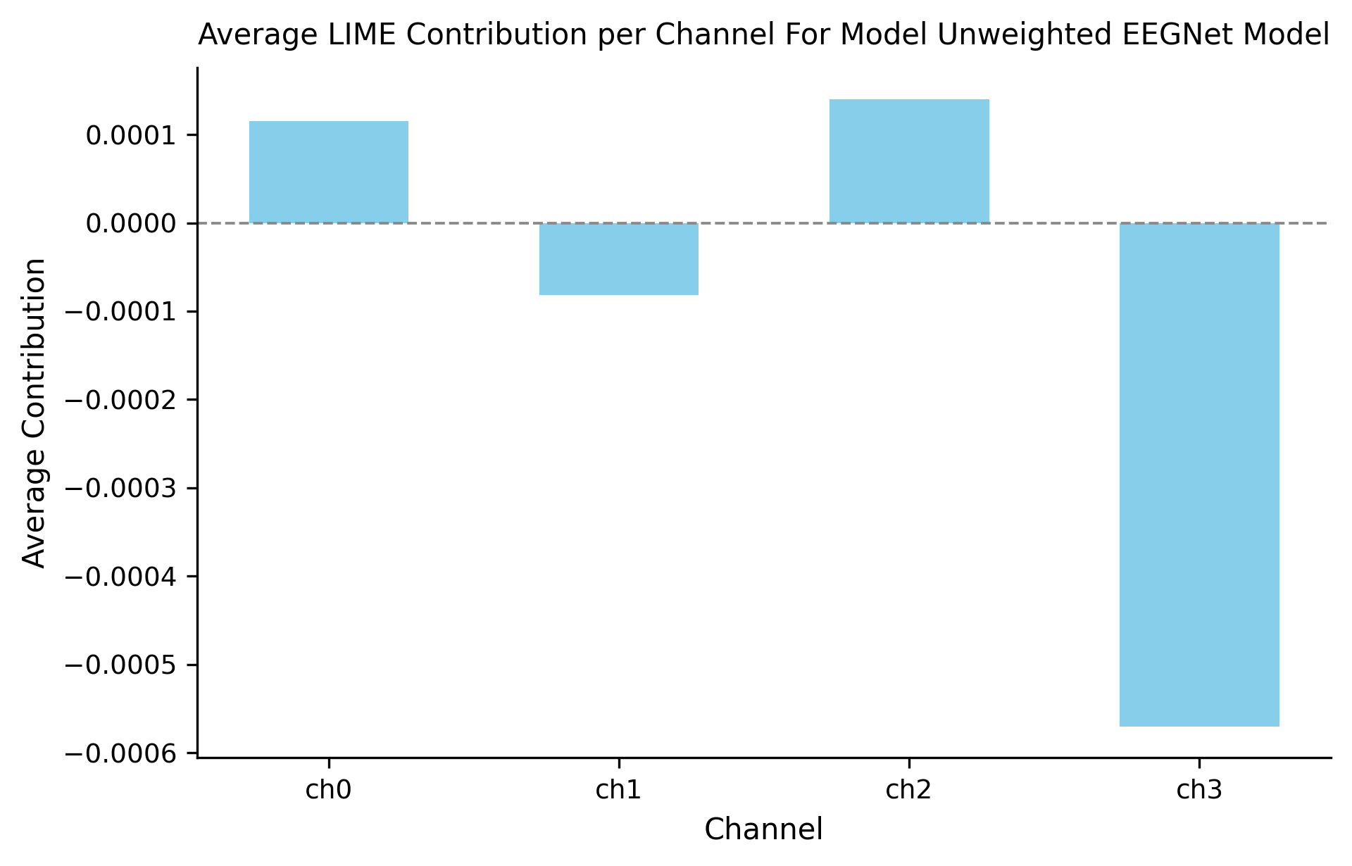
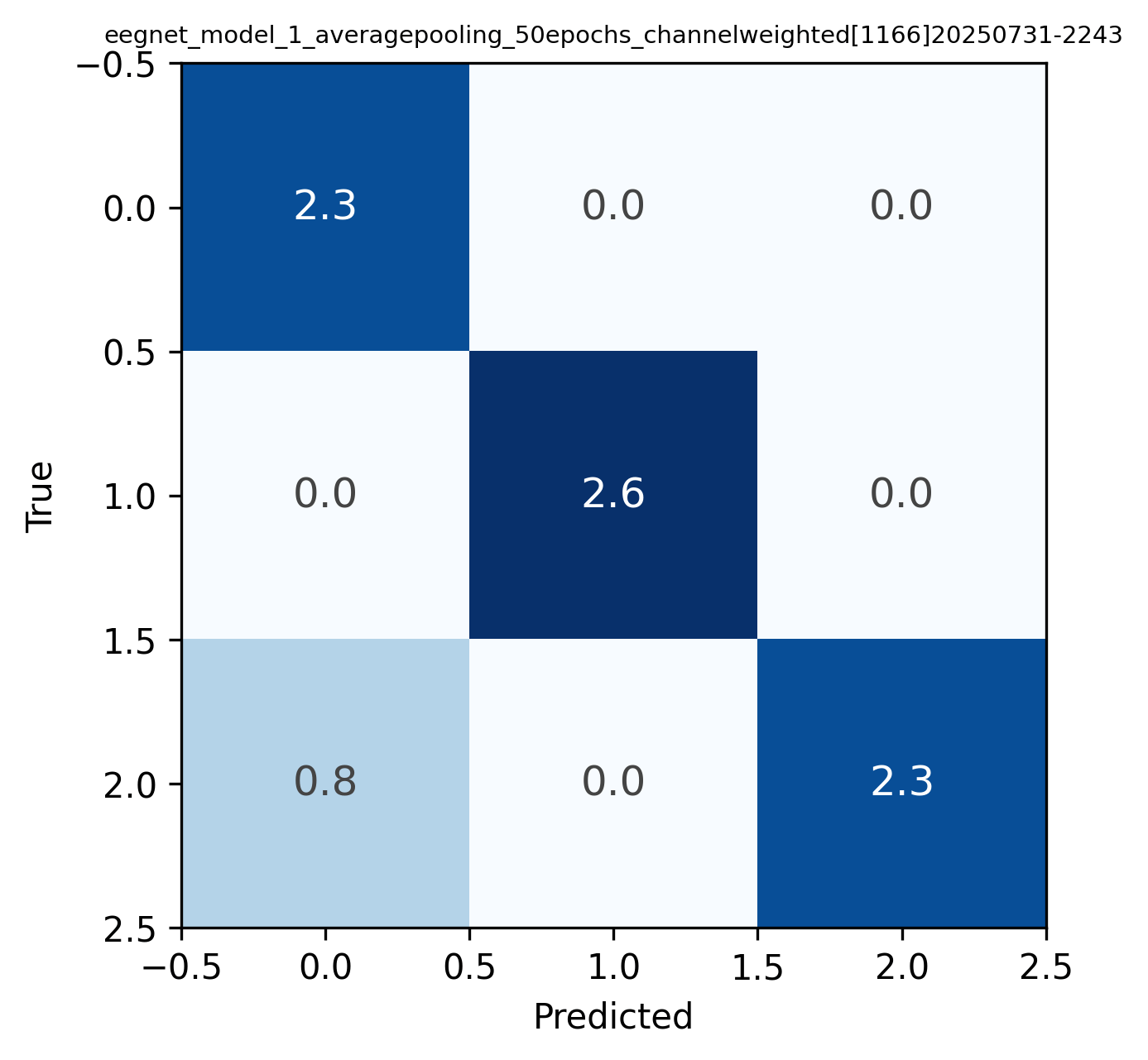
Scalars, w, were applied to solely the training data on channels with artifacts or large negative influence. In doing so, I guide the model in learning relevant patterns and steering away from relying on noise. Many weights were experimented with (see Appendix B: CM 1), but the weights [1, 1, 0.6, 0.6] resulted in the highest accuracy and an increase from the unweighted model (see Figure 4). Weights were applied to channels 1 (TP7) , 2 (TP8) , 3 (F7), and 4 (F8) respectively.
The new learned features and weights were analyzed. This was done in the same manner using LIME analysis. Figure 5 displays the average contribution per channel of the newly weighted model. The newly weighted model no longer depended on artifacts in channel 3 (chan. 2 on figure). With this, the model began to utilize channel 2 (chan. 1 on figure) to a greater degree which was rich in patterns.
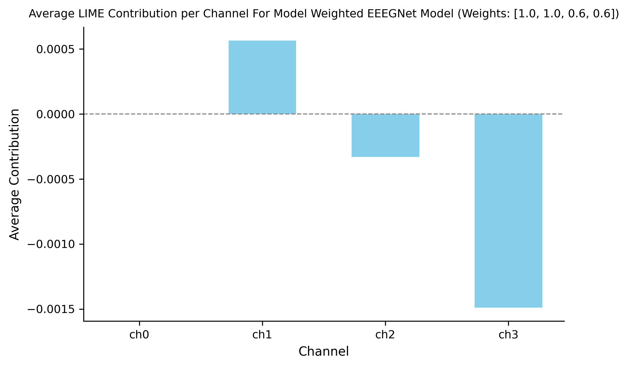
non-artificial channel 2 (chan. 1 on figure) is evident along with a decrease in reliance on artificial channel 3 (channel 2 on figure). Once again, reweighting clearly has an effect in redirecting the model to potentially important channels (especially those farthest away from the eyes).
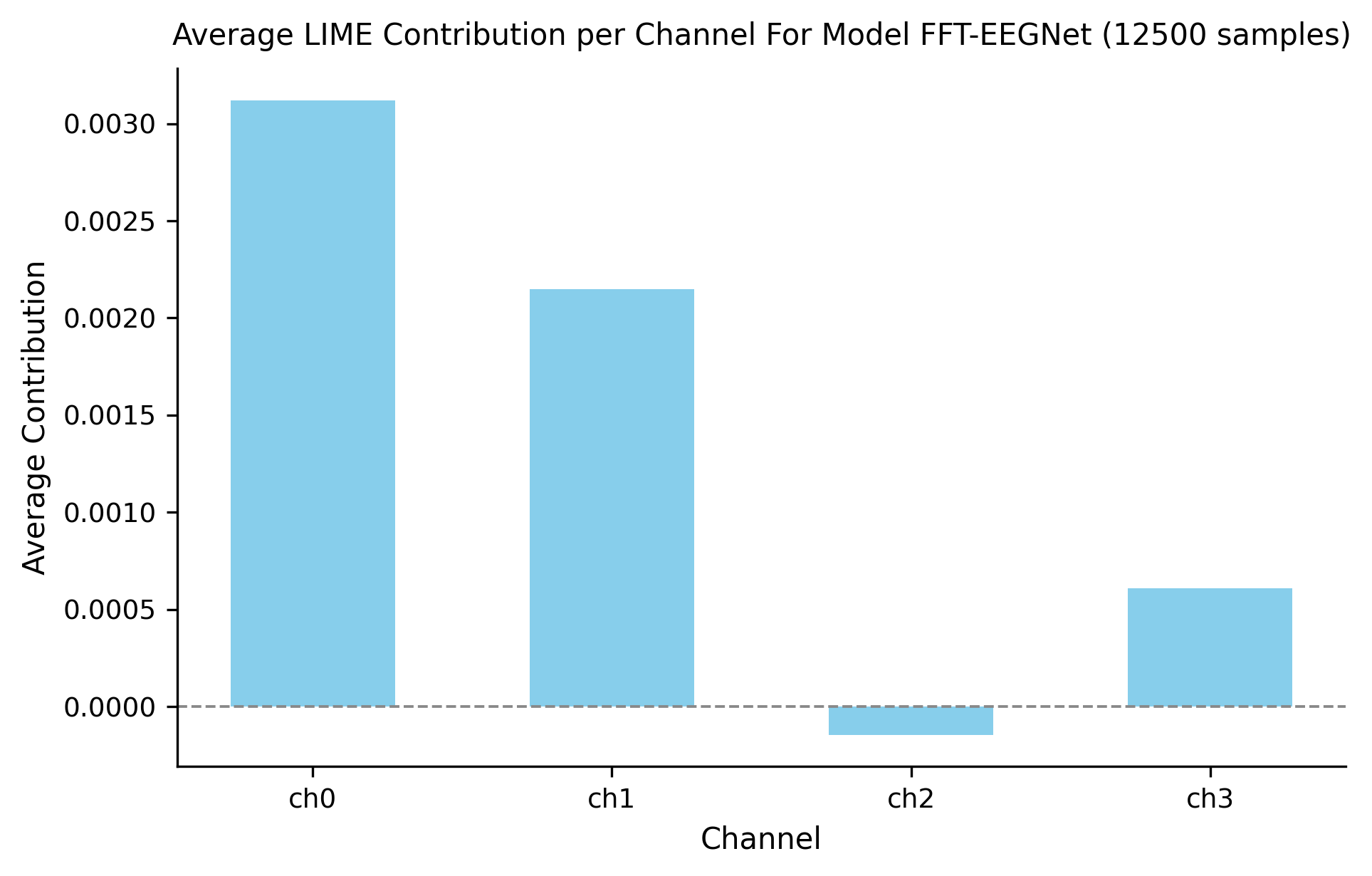
Through extensive weight analysis and subsequent reweighting, accuracies can be significantly improved. This same pipeline was utilized in noun/verb classification in which the same trends arose (see Appendix B: CM 3 and Analysis 1 for more details). While this may be plausible it is often tedious, time consuming and resource intensive. In figure 6 I demonstrate the innate ability of FFT models to more
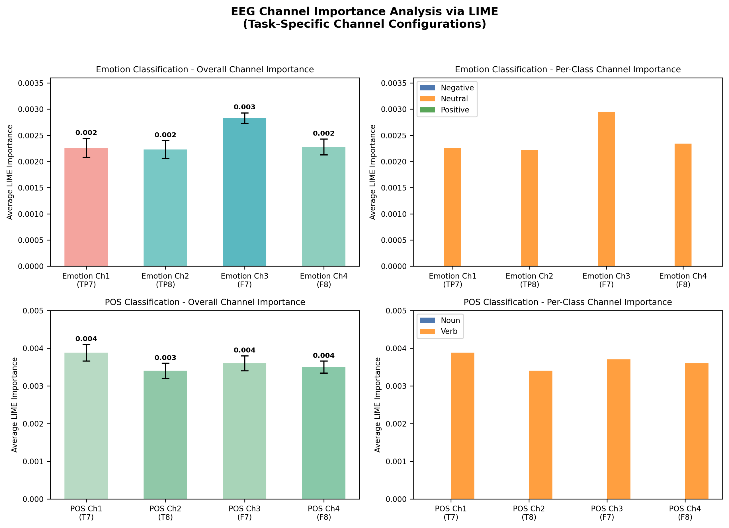
efficiently and accurately rely on correct channels across both emotion and POS tasks (see Figure 7; Appendix B: Analysis 1) The FFT model clearly has correctly relied less on channels 3 and 4 (2 and 3 on the figure). This FFT model accuracy exceeded that of the baseline time-series model by ~9% and the weighted time-series model by ~6%.
Fused Multi-head Model (fine-tuning fusion)
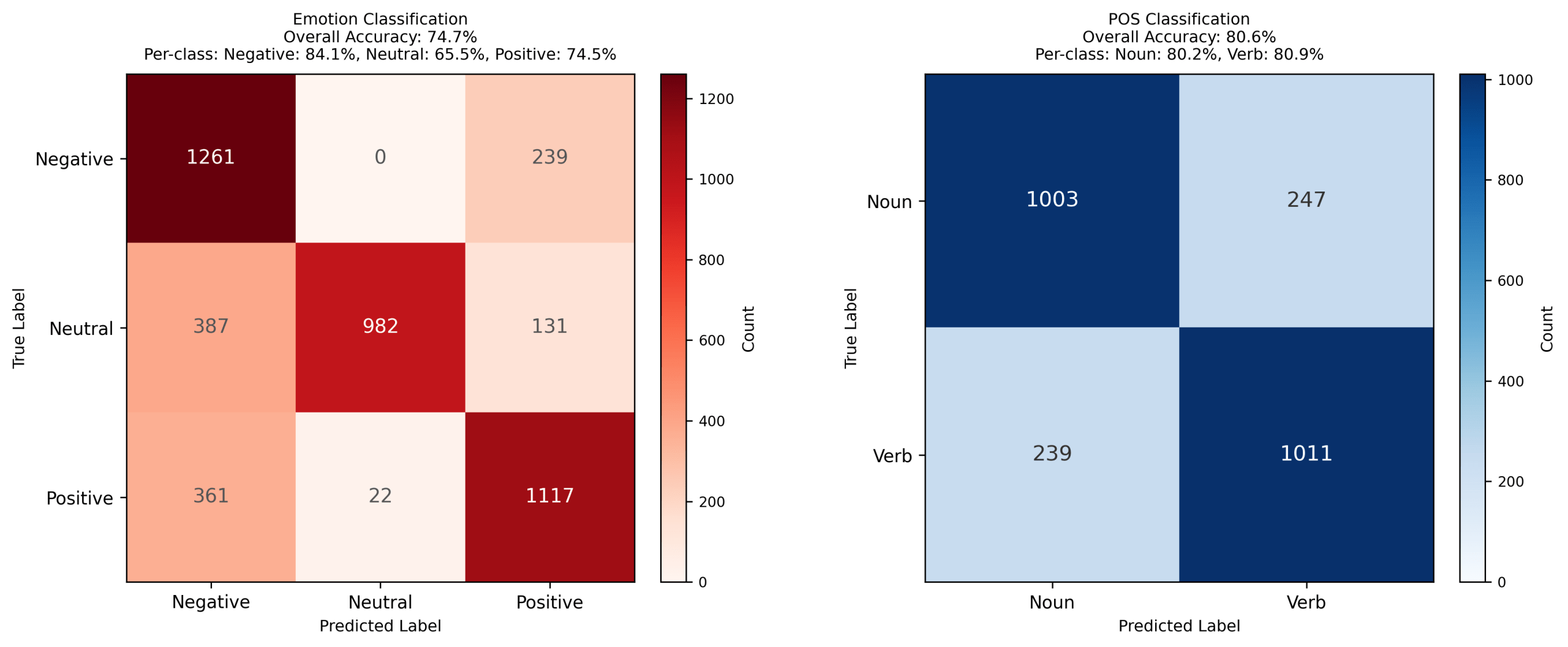
To create an efficient multi-task model without retraining from scratch, using existing FFT models (due to its efficacy demonstrated above), I fused early convolutional encoders from these independently trained single-task FFT models and fine-tuned shared dense layers plus task-specific heads (see methods). The models evaluated in the following figures used early learned weights from the emotion and POS single-task models. These were then concatenated into a fused encoder. In figure 7, the fused model (see Appendix A: Table C1 for architecture) underperformed single-task models (~16% worse on emotion, ~9% on POS; Fig. 7). LIME showed artifact reliance (Fig. 8), and reweighting yielded negligible gains (~0.3%; Figs. 9-10).
Fusing early encoders allows for the reuse of learned spectral and spatial filters and reduces training cost and resource use. The weighted, fused model offered a modest improvement in combined multi-task accuracy while only some decline in per-task performance. However, the futility of reweighting causes a problem in optimizing and boosting accuracies of these types of models. Additionally, it’s clear that the shared representations hinder performance (a common phenomenon in EEG decoding). Brain activity is incredibly distinct and non-stationary (a result of subject differences and a lack of standardization), both among participants and tasks, making a valuable shared representation incredibly difficult to achieve23. Often, as likely in the case of this experiment, the model is unable to distinguish the signals from the representation space. Hence, a new approach to multi-task classification will be explored in the following section.
Embedding-Constrained EEG Architecture
To test whether linguistic structure can inform architecture design, I clustered word embeddings into semantic groups and built specialized branches per group (embeddings were not used at inference). Architecture summary (see Appendix B: Flowchart 2): K = 2 clusters (method = KMeans, embeddings of dimension = OpenAI’s text-embedding-3-small). The embeddings are of dimension 1536 and cosine similarity is used to measure clustering distance. Branches: dynamically adjusted based on clustering results (See Methods & Appendix A: Table A1 for more details).
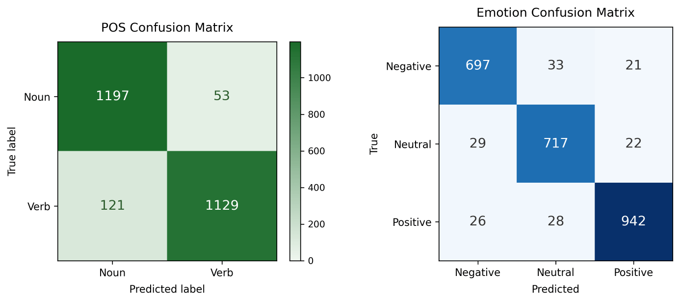
The embedding-constrained model was trained from scratch using FFT data from both emotion and POS tasks (see Results, C), processing EEG inputs in parallel via specialized branches derived from embedding clusters (e.g., emotion, concrete/abstract, noun/verb), each with neuroscience inspired filters tuned to relevant frequencies. Branch outputs are concatenated into a shared layer, enabling the model to learn branch weighting for final classification. With embeddings, it dynamically analyzes stimulus words, leveraging semantic representations, to build these branches, though currently manually designed (automatable via OpenAI API)19. This architecture significantly outperformed baselines and fused models, and matched single-task emotion performance (see Figure 11). It was ~4% better than single-task POS, and ~12.5% better overall than the best multi-head fusion.
Embedding-as-regularizer strategy (alternative)
To contrast with architecture-level embedding usage, I implemented an auxiliary embedding-prediction loss (cosine similarity) to force EEG features toward semantic vectors and evaluated its performance relative to the proposed model. I hypothesized that a loss forcing the model to learn vectors would compete with the EEG loss, resulting in lower accuracies and less learned EEG patterns (and hence an overreliance on embeddings).
This approach dropped accuracy ~20-30% and caused instability/overfitting, supporting architecture-level biases over auxiliary losses.
Summary of mean test accuracies over 100 shuffled evaluations accuracies are reported with 95% Wilson binomial confidence intervals; note: for time-series models, CI will be large due to small testing sizes, but this is mitigated through shuffling and averaging for confidence (see methods).
| Model / Representation | Emotion acc (%) mean | POS acc (%) mean | Combined, mean acc (%) | Task Count |
|---|---|---|---|---|
| Time-series EEGNet | 87.50% 95% CI: 46.48–98.26 | 89.74% 95% CI: 48.9–98.83 | 88.62% | Single task |
| FFT-EEGNet | 95.77% 95% CI: 94.94–96.43 | 93.94% 95% CI: 92.57–95.06 | 94.86% | Single task |
| Time Series + LIME reweight | 90.12% 95% CI: 61.74–98.05 | — | 90.12% | Single task |
| Fused multi-head (with best weights) | 74.70% 95% CI: 73.59–75.72 | 80.6% 95% CI: 79.23–81.8 | 77.65% | Multi-task |
| Embedding-constrained | 94.12% 95% CI: 93.42–94.96 | 93.04% 95% CI: 92.16–93.83 | 93.58% | Multi-task |
| Embedding-regularizer | 64.95% 95% CI: 63.21–66.35 | 73.82% 95% CI: 72.53–75.42 | 69.39% | Multi-task |
Discussion
I introduced and analyzed strategies for semantic decoding from minimal EEG. I introduced FFT data amplification from short FFT snapshots, channel reweighting, fusion for multi-task classification, and finally an embedding-constrained EEG architecture using word embeddings just during design. Under constraints of four channels and 50–100 stimulus words, this model achieved the strongest performance across emotional valence (negative/neutral/positive) and part-of-speech (noun/verb) tasks. FFT-trained models consistently outperformed time-series baselines, highlighting spectral data’s efficacy in data-limited scenarios (see Results and Table 1).
The embedding-constrained gains come from encoding neuroscientifically informed biases into network structure, with specialized branches tuned to certain frequency bands (e.g., delta/theta/alpha for emotion; beta/gamma for noun/verb20. This builds on current optimization techniques for EEG architectures18. In contrast, the “embedding-as-regularizer” approach showed poor accuracy due to optimization conflicts in noisy data, underscoring the advantages of simpler biases over multiple losses. This follows general intuition of Ocaam’s Razor: the simplest solution is often the best or in this case, overcomplicating the loss function leads to worse results. Additionally, because a loss function is intended to guide the model, having multiple “guides” is often detrimental and leads to inevitable confusion. EEGNet’s design allowed for an explainability pipeline (depthwise/separable filter inspection + LIME) that identified artifactual channels and guided reweighting for accuracy improvements2.
Several limitations deserve highlighting; they are enumerated in order of importance and/or affect. First are the FFT amplification risks bias despite precautions. Such precautions were employed here due to small datasets, single-participant scope, and task-specific goals, but further steps should be taken to mitigate this potential issue for larger, more diverse datasets. Second, lacking cross participant testing limits inference strength. Third, consumer EEG hardware (OpenBCI Ganglion) adds noise, adding practicality, but limiting generalizability. Fourth, branch designs depend on embedding models and clustering, potentially causing less ideal architectures (as evidenced by small POS gains (~2%) versus emotion (~7%)). Fifth, because EEG signals exhibit strong individual variability, solely within-participant evaluation may inflate decoding accuracy by allowing models to exploit participant specific signal traits/patterns rather than generalizable representations24. To this end, I must limit the broader interpretation of these results as they may arise solely as a product of the participants used8. While this limitation can be seen as only a negative, it does also introduce a question regarding the future potential of lightweight, easily adaptable models for certain tasks or participants. Finally, while LIME analysis is a commonly employed technique to view features, it also is known that it can exhibit instability and/or volatility25. This consequence has the potential to distort or diminish the channel attribution analysis. With this in mind, it would be beneficial to explore other interpretability methods or correct the measurements based on known instability.
This work demonstrates a low-cost, small-scale BCI proof-of-concept for semantic decoding. Utilizing few channels and limited trials, it leverages linguistic knowledge for a compact architecture and employs FFT data amplification when generalization is not required.
Recommended next steps: replicate with diverse groups to assess generalization and fine-tuning. Explore alternate clustering methods and semantic tasks for flexibility. Develop methods for across subject accuracy. Optimize electrode placements and conduct real-time evaluations. Finally, reduce data amplification reliance for larger datasets.
Conclusion
FFT sampling generated larger training sets with little expected leakage, showing better performance over time-series inputs. Reweighting provided single-participant gains, while fused multi-head models enabled decent multi-task accuracy. The embedding-constrained architecture delivered strongest accuracies (~93.5%), requiring only EEG at inference and showing strong performance across tasks with quick, resource light training. These findings illustrate how neuroscience informed biases and FFT features can reduce data and hardware demands for semantic BCI’s. Future efforts should expand experimental size, add more specialized pathways, automate cluster analysis, reduce reliance on amplification, and enable real-time decoding.
APPENDIX
See the detailed appendix here: https://github.com/benski20/EEG_RESEARCH_APPENDIX.git
Acknowledgments
I would like to acknowledge my mentors, Mr. Clement and Dr. Brandao for their support, along with the reviewers for their thoughtful comments.
Consent to Participate
All participants involved in this laboratory exercise provided their consent to participate voluntarily. The experiment posed no physical, ethical, or privacy risks, and all members contributed equally to data collection and analysis.
Funding Declaration
This work received no specific grant or financial support from any funding agency, commercial entity, or not-for-profit organization.
Data Availability and Materials
The data that support the findings of this study are not publicly available due to participant privacy and protection requirements. Data may be made available upon reasonable request to the corresponding author, subject to institutional approval and ethical considerations.
References
- N. Hollenstein, C. Renggli, B. Glaus, M. Barrett, M. Troendle, N. Langer, C. Zhang. Decoding EEG brain activity for multi-modal natural language processing. Frontiers in Human Neuroscience. Vol. 15, pg. 659410, 2021, https://doi.org/10.3389/fnhum.2021.659410. [↩]
- V. J. Lawhern, A. J. Solon, N. R. Waytowich, S. M. Gordon, C. P. Hung, B. J. Lance. EEGNet: A compact convolutional neural network for EEG-based brain-computer interfaces. Journal of Neural Engineering. Vol. 15, pg. 056013, 2018, https://doi.org/10.1088/1741-2552/aace8c. [↩] [↩] [↩]
- T. M. Mitchell, S. V. Shinkareva, A. Carlson, K. M. Chang, V. L. Malave, R. A. Mason, M. A. Just. Predicting human brain activity associated with the meanings of nouns. Science. Vol. 320, pg. 1191–1195, 2008, https://doi.org/10.1126/science.1152876. [↩]
- F. Pereira, B. Lou, B. Pritchett, S. Ritter, S. J. Gershman, N. Kanwisher, M. Botvinick, E. Fedorenko. Toward a universal decoder of linguistic meaning from brain activation. Nature Communications. Vol. 9, pg. 963, 2018, https://doi.org/10.1038/s41467-018-03068-4. [↩]
- L. Wehbe, B. Murphy, P. Talukdar, A. Fyshe, A. Ramdas, T. M. Mitchell. Simultaneously uncovering the patterns of brain regions involved in different story reading subprocesses. PLoS ONE. Vol. 9, pg. e112575, 2014, https://doi.org/10.1371/journal.pone.0112575. [↩]
- M. Schrimpf, I. A. Blank, G. Tuckute, C. Kauf, E. A. Hosseini, N. Kanwisher, J. B. Tenenbaum, E. Fedorenko. The neural architecture of language: Integrative modeling converges on predictive processing. Proceedings of the National Academy of Sciences. Vol. 118, pg. e2105646118, 2021, https://doi.org/10.1073/pnas.210564611-8. [↩]
- Y. Roy, H. Banville, I. Albuquerque, A. Gramfort, T. H. Falk, J. Faubert. Deep learning-based electroencephalography analysis: A systematic review. Journal of Neural Engineering. Vol. 16, pg. 051001, 2019, https://doi.org/10.1088/1741-2552/ab260c. [↩]
- Y. Wang, H. Liu, Y. Wang, C. Xuan, Y. Hou, S. Feng, H. Liu, Y. Liao, Y. Wang. Progress, challenges and future of linguistic neural decoding with deep learning. Communications Biology. Vol. 8, pg. 1071, 2025, https://doi.org/10.1038/s42003-025-08511-z. [↩] [↩] [↩]
- P. Bashivan, I. Rish, M. Yeasin, N. Codella. Learning representations from EEG with deep recurrent-convolutional neural networks. arXiv preprint. https://arxiv.org/abs/1511.06448, 2015. [↩] [↩]
- B. Blankertz, G. Dornhege, M. Krauledat, K. R. Müller, G. Curio. The non-invasive Berlin Brain–Computer Interface: Fast acquisition of effective performance in untrained subjects. NeuroImage. Vol. 37, pg. 539–550, 2007, https://doi.org/10.1016/j.neuroimage.2007.01.051. [↩]
- A. Goyal, Y. Bengio. Inductive biases for deep learning of higher-level cognition. Proceedings of the Royal Society A. Vol. 478, pg. 20210068, 2022, https:// doi.org/10.1098/-rspa.2021.0068. [↩]
- R. Maskeliunas, R. Damasevicius, I. Martisius, M. Vasiljevas. Consumer-grade EEG devices: are they usable for control tasks? PeerJ. Vol. 4, pg. e1746, 2016, https://doi.org/10.7717/peerj.1746. [↩] [↩]
- E. Gkintoni, A. Aroutzidis, H. Antonopoulou, C. Halkiopoulos. From neural networks to emotional networks: A systematic review of EEG-based emotion recognition in cognitive neuroscience and real-world applications. Brain Sciences. Vol. 15, pg. 220, 2025, https://doi.org/10.3390/brainsci15030220. [↩] [↩]
- P. Sun, G. K. Anumanchipalli, E. F. Chang. Brain2Char: A deep architecture for decoding text from brain recordings. Journal of Neural Engineering. Vol. 17, pg. 066015, 2020, https://doi.org/10.1088/1741-2552/abc742. [↩]
- S. K. Wandelt, D. A. Bjånes, K. Pejsa, B. Lee, C. Liu, R. A. Andersen. Representation of internal speech by single neurons in human supramarginal gyrus. Nature Human Behaviour. Vol. 8, pg. 1136–1149, 2024, https://doi.org/10.1038/s41562-024-01867-y. [↩]
- E. Lashgari, D. Liang, U. Maoz. Data augmentation for deep-learning-based electroencephalography. Journal of Neuroscience Methods. Vol. 346, pg. 108885, 2020, https://doi.org/10.1016/j.jneumeth.- 2020.108885. [↩] [↩]
- Y. Huang, J. Zheng, B. Xu, X. Li, Y. Liu, Z. Wang, H. Feng, S. Cao. An improved model using convolutional sliding window-attention network for motor imagery EEG classification. Frontiers in Neuroscience. Vol. 17, pg. 1204385, 2023, https://doi.org/10.3389/fnins.2023.1204385. [↩]
- D. Aquino-Brítez, A. Ortiz, J. Ortega, J. León, M. Formoso, J. Q. Gan, J. J. Escobar. Optimization of deep architectures for EEG signal classification: An AutoML approach using evolutionary algorithms. Sensors. Vol. 21, pg. 2096, 2021, https://doi.org/10.3390/s21062096. [↩] [↩]
- T. He, M. A. Boudewyn, J. E. Kiat, K. Sagae, S. J. Luck. Neural correlates of word representation vectors in natural language processing models: Evidence from representational similarity analysis of event-related brain potentials. Psychophysiology. Vol. 59, pg. e13976, 2022, https://doi.org/10.1111/psyp.13976. [↩] [↩]
- F. Pulvermuller, H. Preissl, W. Lutzenberger, N. Birbaumer. Brain rhythms of language: nouns versus verbs. European Journal of Neuroscience. Vol. 8, pg. 937–941, 1996, https://doi.org/10.1111/j.1460-9568.1996.tb01580.x. [↩] [↩]
- Y. Zhang, G. Yan, W. Chang, W. Huang, Y. Yuan. EEG-based multi-frequency band functional connectivity analysis and the application of spatio-temporal features in emotion recognition. Biomedical Signal Processing and Control. Vol. 79, pg. 104157, 2023, https://doi.org/10.1016/j.bspc.2022.104157. [↩]
- S. Geng, N. Molinaro, P. Timofeeva, I. Quiñones, M. Carreiras, L. Amoruso. Oscillatory dynamics underlying noun and verb production in highly proficient bilinguals. Scientific Reports. Vol. 12, pg. 764, 2022, https://doi.org/10.1038/s41598-021-04737-z. [↩]
- R. T. Schirrmeister, J. T. Spring- enberg, L. D. J. Fiederer, M. Glasstetter, K. Eggensperger, M. Tangermann, F. Hutter, W. Bur- gard, T. Ball. Deep learning with convolutional neural networks for EEG decoding and visua- lization. Human Brain Mapping. Vol. 38, pg. 5391–5420, 2017, https://doi.org/10.1002/hbm .23730. [↩]
- P. Singh, A. Sharma, P. Pandey, K. Miyapuram, S. Raman. EEGVid: Dynamic vision from EEG brain recordings, how much does EEG know? arXiv preprint. https://arxiv.org/abs/2505.21385, 2025. [↩]
- P. Knab, S. Marton, U. Schlegel, C. Bartelt. Which LIME should I trust? Concepts, challenges, and solutions. arXiv preprint. https://arxiv.org/abs/2503.24365, 2025. [↩]


