Analyzing Patterns within a Song’s Musical Characteristics through Machine Learning

Abstract

Musical genres are characterized by various distinct audio features, but the quantitative relationships between these features and genre classifications remain underexplored. The purpose of this experiment is to identify important relationships and analyze patterns between features, genre, and audio data through machine learning models in two separate experiments. The first experiment tested the validity of waveforms for regression tasks. Waveforms are less commonly used and this experiment focuses on introducing them to be used in machine learning tasks. The second experiment addresses the difficult task of genre classification and does so with a tensor of numerical feature values used  to classify a song into one of 5 genres: hip-hop, rock, dance/electronic, pop, and R&B. For the regression task, a normalized tensor containing waveform signals found for different songs from a dataset was passed into a deep linear neural network with convolutional layers. This predicts various numerical features such as tempo or the danceability of a song. Meanwhile for genre classification, random forest and neural network architectures were used for single class and multi-class prediction based on the likelihood of a song sharing common features associated with a genre. The same numerical features provided in the dataset were used as inputs. The findings revealed that solely waveform-based approaches are insufficient as seen by the model’s inability to generalize and so other types of higher-level depictions of audio should be leveraged to predict numerical features of a song which are often semantic. The multi-output regression model had a testing loss of 0.0385 and R²-score of -0.25 signifying the inability to capture essential patterns from a waveform representation. The random forest performed better compared to the neural network for the genre classification task but there was large overlap between genres and weak feature discrimination during analysis with an F₁-score of 0.60. In the future, genre classification should be approached not just through numerical features but with other cultural or auditory context as well and more richer audio representation is necessary for regression tasks like this.

Introduction

Music and its various characteristics have the ability to change the mood and feelings of its listeners. As such, music is not only a form of entertainment and relaxation, but also can be used as forms of therapy and strengthening one’s mental health. Music directly affects one’s bodies, proving to be physically and mentally beneficial. A recent study by Van Edwards in 2024 shows that when slow music is played, the bodily reaction follows suit¹. Specifically, our brain adjusts our heart rate to slow down and correlate with the music. Different types of music have different effects as seen by this example. Faster, louder songs have the capability of making one feel active while slower, soothing songs make one feel at ease. The differences in reactions that one can have from different types of music prove the diversity of music itself. 

This diversity is not blindly created, rather, it is formed with a certain intent by the artist and numerous concrete features. These features, like energy or tempo, work hand in hand to create the best sound quality and convey certain feelings and so in order to create music that is the most effective in conveying these emotions, many artists use musical characteristics in similar configurations. 

This project aims to understand how these features make music something impactful and cohesive by examining two aspects of music through separate experiments: the ability of a model to recognize patterns in the features mentioned earlier such as valence, energy, and tempo within a waveform and in a song’s genre. In order to do so, this project utilized machine learning to see if a model could find patterns which meant there had to be a way to feed the model the sounds found in the music digitally. While spectrograms are mainly used for audio-based deep learning, this project intends to explore how effective waveforms, a different way of representing audio data visually, are during audio-based deep learning to expand on the field and allow for different methodologies in future audio-based deep learning applications. The common power spectrograms do not retain phase information and other temporal information². Waveforms describe this temporal information and are much more accessible and readable to humans. These benefits could possibly be leveraged if waveforms were used in audio based machine learning applications. Previous literature has addressed gaps related to many issues of musical feature extraction and musical classification by converting audio data into different forms of data such as spectrums³. Similarly, this project aims to use the primitive visualization of audio, waveforms, to tackle musical feature extraction specifically for numerically qualified features. Using features from songs such as danceability or energy, this project will also tackle genre classification using these features since feature extraction directly from audio signals takes away from the symbolic and cultural aspects of songs which are often important in genre classification. Genre classification is a subjective task and so this project attempts to address that by using both objective and subjective songs features such as tempo and danceability. These features could define what makes a song one genre over another. Using the waveform, visual representation of certain aspects of audio data, of a song to predict its musical characteristics, along with a neural network to learn patterns within the audio data, it will be possible to determine the true extent to which waveforms can be used for audio-based deep learning tasks. Furthermore the song’s numerical features will be used to attempt to classify genre and further complete the genre classification task. Both of these experiments will quantify and observe the interplaying relationships in a song’s features, genre, and waveform representation.

Literature Review

Music Information Retrieval

Music Information Retrieval (MIR) refers to the use of audio content analysis to retrieve or categorize music⁴. Processes like feature extraction and machine learning are used to perform tasks such as genre classification and recommendation systems recently for MIR. For example, using music information retrieval techniques, recommendation systems are able to retrieve certain types of songs and certain genres for the user based on previous observations making machine learning and the digitization of modern music especially supported in this field. MIR uses image, video, audio, and multimodal analysis techniques to retrieve music information. Content-based audio retrieval, a form of MIR, in recent times focuses on reducing a semantic gap, human perceptions based on cultural context, emotion, and motifs featured in music that machines are not able to comprehend. It involves a common architecture featuring three modules: input, query, and retrieval⁵. Input involves feature extraction from the given input and then during the query module, a query is formulated based on the input from which common features are extracted as well and put through a query database which contains numerous objects. Finally, during retrieval the features are both compared to find a common object from the database which is then retrieved. Feature extraction, a salient phase of machine learning processes, in audio-based deep learning can involve extracting musical characteristics such as pitch, timbre, or melody to perform tasks like genre classification. A common and important technique within MIR is audio signal processing often also used for audio classification tasks. This involves actions like compression or segmentation of different auditory representations with time-frequency representations in order to better prepare the sample for things like feature extraction or classification⁶. Waveforms could, as a form of audio signal representation, be more suitable for certain aspects of digital audio processing like direct manipulation since it is a clear visualization of the change of a value over time pertaining to the audio.

Genre

Genres are categories that describe the overall musical characteristics of a song and while they can be subjective, there are usually several key indicators found in musical features that indicate a certain genre. The music found in a specific genre follows a particular cultural pattern or shared sound, and it’s how songs often get classified into their respective genres⁷. Therefore classifying a song’s genre through its features to determine how strongly the genre correlates to a song’s numerical characteristics can prove insightful as genre allows expression and symbolism to listeners. Genre classification is a key topic in music information retrieval and is being addressed with machine learning techniques in recent times. Recent studies have shown that approaches like CNN based image classifiers can classify genre to a greater degree than other forms like feature-engineering models proving the effectiveness of neural networks in recent times⁸. Due to its subjective nature, genre classification is hard to get accurate data for a model to train off of and is usually approached in five forms: i) audio content-based, (ii) symbolic content-based, (iii) lyrics-based, (iv) community meta-data based, and (v) hybrid approaches⁹. Usually supplementary features of a song such as album covers or music videos are used to determine genre but nonetheless genre classification is an important, difficult task due to their not being pre-existing taxonomies. Genre classification can be done in many ways such as with unsupervised learning due to genres not having predefined rules or more commonly and recently, supervised learning in which a model learns the rules for genre classification based on pre-labeled datasets. However, despite many attempts, genre classification has not been able to achieve higher than 60% precision for large genre variety without the use of multimodal analysis  but has gone to 80% for low ranges of genre⁴. By using extracted features depicting the characteristics of a song, there can be an audio-content based manner of predicting genre if clear patterns are found within these features since feature values of certain ranges could often correspond to a certain genre that fits the same pattern. In a previous experiment that used waveform extracted features to predict genre, the best model was able to predict with 68.5% accuracy on unseen data¹⁰. Therefore, a varying approach could involve less technical audio features. For example, the study done by Henrique used features such as spectral centroid while more perceptual and behavioral features such as danceability could be used to address cultural or symbolic genre classification gaps.

Waveforms

Music can be represented digitally in numerous ways through audio data. Audio data represents analog sounds in a digital form, preserving the main properties of the original¹¹. Visually, raw audio data in a song can be depicted as a waveform, which are graphs of a signal over time with amplitude. Audio data has three dimensions: time period (how long sounds last), amplitude (volume of sound), frequency (number of vibrations in a certain time)¹². Waveforms, spectrums, and spectrograms are able to depict all these dimensions but in different ways and fourier transforms are what are used to extract and convert audio data from time-based to frequency-based¹³ or from waveform to spectrogram in the case of a short-time fourier transform since waveforms are unable to properly express signal properties and similarities unlike spectrogram⁵. Fourier transforms are necessary since audio is often best represented with both time and frequency rather than only the time domain.

Fourier transforms are the key for music recognition softwares such as Shazam which often use short-time fourier transforms to transform an input waveform to spectrograms for greater ease when predicting for audio-based deep learning. This takes computational resources, however. Audio-based deep learning is used for segmentation (audio separation), text-to-speech, and audio classification¹⁴. For audio classification during audio-based deep learning, multiple connected linear layers are often used¹⁴. For purposes like mixing, enhancing, and manipulating pieces of audio data, waveforms are most commonly preferred and there could therefore be many benefits of using waveforms to extract audio data and for analysis using audio-based deep learning. Furthermore, a deep neural network, WaveNet, creates raw audio as a waveform by modeling waveforms and is used in applications such as text-to-speech¹⁵ proving the primitive importance and flexibility of waveforms as a form of visualizing audio data. However, this results in a trade-off of losing the frequency domain. This simplification of audio data from the high dimensionality of spectrograms could possibly reduce the aforementioned semantic gap between machine and human. 

Data Description/Analysis

This project uses the “Top Hits Spotify from 2000-2019” dataset on Kaggle. This dataset contains audio statistics of the top 2000 tracks on Spotify from 2000-2019 through 18 characteristics that describe the qualities of the song¹⁶.

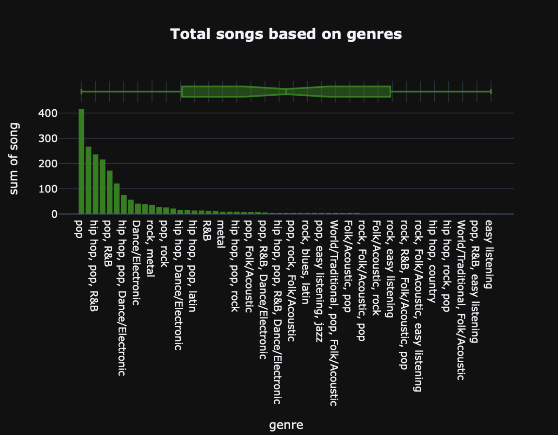
Each song is categorized by genre with many of the songs being classified with two or three genres. Observing the dataset, most of the songs were under the genre pop, whether pop was their only genre or it was pop in addition to other genres. Songs only classified as pop made up 21% of the entire dataset, which is quite substantial. Other notable genres in the dataset include: hip-hop , dance/electronic, rock, and R&B which are the genres that this model will specifically focus on.

Figure 1 shows the most common genres with genre on the x axis and the number of songs categorized into that genre on the y-axis as a bar graph.

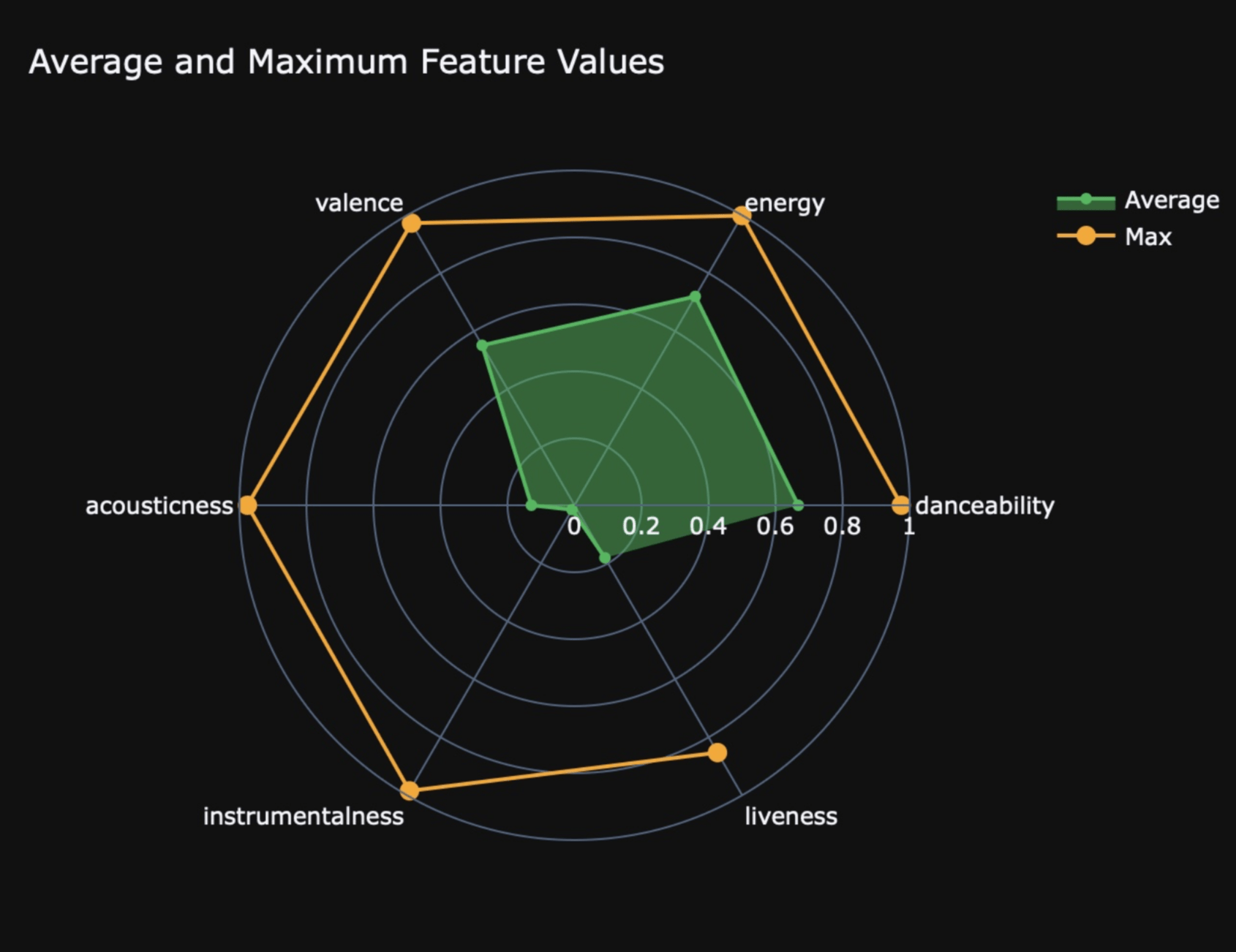
In addition to genre, each song was assigned features with their own unique values. For example, each song has: a tempo which quantifies the speed of that song in beats per minute, a valence which conveys the relative musical positiveness of that song, and an energy that perceives the activeness of that song. Similarly, there are many other different features that all contribute their own qualities to the creation of a song and have been assigned values by the dataset. To the benefit of this experiment, most of the features are numerical values often between 0 and 1 (See Figure 2). 

Figure 2 shows the 6 features with values from 0-1 and the average/max values for each feature. Every feature’s max possible value was 1.0 as seen by the orange dots. But for example, the average danceability value was a little above 0.6 as seen by its corresponding green dot while liveness average value across the entire dataset was just shy of 0.2.

However, the dataset did not include audio or waveform data of each song which meant they had to be manually collected by downloading and converting mp3s from the internet archive. As mentioned, there were many more songs under the genre pop than others which would create an imbalance for the model as it is learning. In order for the model to learn effectively and without bias, it needs to be exposed to every class equally. So if pop was shown more often, it would be more biased in predicting pop because that is what it is used to. Finally, since some songs had multiple genres this could complicate the training and learning process so only one genre was chosen for each song in order to create a class-balanced dataset by prioritizing uncommon genres such as dance/electronic over genres like hip-hop when it was classified as both in the dataset. However, as will be mentioned further, this led to problems surrounding over-saturation of genres; since genres like hip-hop and pop were being dropped as labels to the model but their characteristics were still present, the neural network could still pick up on these characteristics and somewhat inaccurately predict.

Methods/Experiment Design

Once the dataset was chosen, songs were handpicked from the dataset and preprocessed in order to integrate them into the colab, a Jupyter notebook that allows users to write and run python code for data analysis and machine learning easily. This process was done by searching through the dataset for a song with one or more of the desired genres (pop, hip-hop, R&B, dance/electronic, or rock) to ensure that there would not be a class imbalance between genres and each genre would have a similar amount of songs. Only five genres were used as previous research has shown that genre classification is able to achieve high precision with a low range of genres to choose from. Next, an mp3 version of the song was downloaded from the Internet Archive and other online resources to then be converted into a WAV file so that it would be compatible with pytorch and more specifically, torchaudio. Torchaudio is a library for audio processing that allows me to store audio data as tensors which can be easily manipulated. It was also used to create the model and for training (Rangwala, 2021). This is done in order to extract the waveform (see Figure 3) and raw audio data. WAV files were uploaded into the colab notebook and initialized into a variable through the torchaudio.load() function. Each song was split between training or testing. With around 70 songs for training and 30 songs for testing creating a 70-30 split.

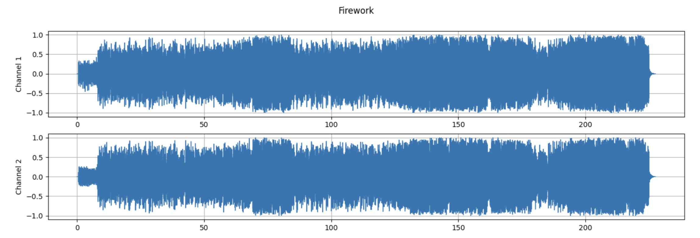
Figure 3 shows how the audio data of a song is visualized through a waveform. The length of the song is on the x-axis and amplitudes of the waves are on the y-axis. This is shown for each channel of the song (like the right and left audio from a headphone).

Predicting Musical Characteristics from Waveform Data

In this experiment, models were created based on an overarching model class for each feature which took as their input, a tensor representing the raw audio data of the song as a tensor and outputs a prediction of that song’s chosen musical characteristics as a numerical value (e.g. tempo, valence, energy, danceability) based on training various weights and biases. These weights, which determine the effect of certain inputs to the resulting output, are determined by iterative training and optimization of the model class. The waveform was passed in as a tensor because tensors are much easier to work with in pytorch; the data held at each tensor index was the amplitude of the function. These values were normalized to a range of 0 to 1 for making the model train easier and more generalizable. After each iteration of training, loss is calculated between the data and predictions using, in this case, the mean squared error loss equation which is shown in section 4.1.1,  and the learning algorithm optimizes the weights accordingly to get the most accurate predictions and therefore most accurate model based on the model class. First, functions were created to track all of the songs and create a tensor with each of the values for a chosen feature to store as the true labels in order to compare with the model class’s predicted values for the loss function. This is how the models learn and optimize during training and how the loss is calculated during testing. So, if ‘tempo’ was passed into the function, this function would return a tensor containing the tempo value for each of the songs downloaded in the training or testing split. Most of the features were values between 0 and 1 but some like ‘tempo’ or ‘loudness’ had to be normalized to the range [0, 1] for improved performance. 

Functions for obtaining the raw audio data as a tensor were also created so they could be used with the tensor of the feature values. To do this, audio data from each channel of the waveform was represented as a single tensor using their mean. Due to varying song length, only a standardized section of 1000 signals for each song was passed through as input thus making the tensor/input length 1000 values. Furthermore, since the entire song was not being used, this allowed for data augmentation in which three different sections were taken as input for each waveform instead of only one. So while only 100 songs’ waveforms were being used, three different sections, each 1000 signals, could be taken from a single waveform making up 300 unique data points after data augmentation with 210 being for training and 90 being for testing.  A deep convolutional neural network model class was created to predict features; the feature value(s) was the output and the input was waveform and audio data from a standardized portion of the song. The approach with each specified feature being trained as a model was condensed to a single multioutput regression neural network model class based on a guide to audio classification and regression with the PyTorch library by Medium¹⁹. It follows the same architecture but utilizes scikit’s multi-output regressor which was wrapped by the original pytorch neural network architecture. This multi-output structure was beneficial in simultaneously predicting several target features using the same inputs and model architecture. The deep model architecture involved five convolutional, relu, pool layers stacked on each other followed by four linear, relu, dropout layers for regularization. The final kernel of the convolutional layer was flattened to allow it to be accessible by the linear layers. This architecture featured two key sections: a convolutional base for feature extraction within the waveform and multiple other layers for mapping these extracted features to predictions. Sci-kit was used for making a custom multioutput regressor wrapper and it was under a pytorch framework. For the first section (convolutional feature extractor), the input was a 1D tensor of normalized values between 0 and 1 representing the 1000 signals. Therefore, a 1D convolutional layer using Pytorch’s neural network capabilities was used to process the data through kernels (filters that detect patterns within a local section of the data). For this specific architecture there were five convolutional layers that kept increasing the number of kernels to learn a larger array of patterns (after each layer, the model combines previous features to learn more complex patterns. After each layer was relu activation for ensuring there are non-linear patterns being learned and pooling for improving computational cost and reducing the number of dimensions so that the model can be more generalizable for small shifts in the input and not overfit which was a common problem during the training. Next was the regression layers which involved the final, flattened output of the convolutional layers and slowly reducing the number of dimensions it was mapped to until the final output returns the values for each specified feature. Relu activations were used after each linear layer and so were dropout layers for regularization to prevent overfitting further by randomly disabling some features. Finally, multioutput was done through sci-kit learn library by fitting one regressor for each target variable. In our setup, the base estimator encapsulates the defined deep convolutional network using the architecture described above. During training, for each target feature, a separate instance of the base estimator is trained on the input waveform data (X) and the corresponding single target feature (y[:, i]). During prediction, each trained estimator predicts its assigned target, and the MultiOutputRegressor combines these predictions into a single multi-output prediction.

This architecture allows the model to learn a rich representation of the audio waveform through the convolutional layers and then use this representation to predict multiple song features simultaneously, leveraging the capabilities of both deep learning and the convenient multi-output handling provided by scikit-learn. The algorithm, ADAM (Adaptive Moment Estimation) was used as the optimization and it allows for better performance and speed when using gradient descents for calculating efficient weights and biases that get the lowest loss. It also is much more lenient when it comes to choosing hyperparameter values such as learning rate and batch size which made it much more manageable to work with. Hyperparameter values were chosen from a search space through gridsearchcv based on initial arbitrary values, however, changes in hyperparameter values had minimal effects on the overall model. The hyperparameter values also included input, output channels and kernel size for the convolutional layers.

The batch sizes were 64 (one batch was the entire training set) because there were not too many songs in the training set. The learning rate of 0.001 was found to work best after running tests with various other learning rates. Although altering the learning rate didn’t change much as the models had enough time to converge with 100 epochs regardless of learning rate. Training functions were created and a mean squared error loss was leveraged to optimize during training since the models were based partly on linear regression. The equation for mean squared error is shown below in section 4.1.1 and minimizing the output loss was the purpose of the ADAM optimizer and after each epoch, it adjusted the model accordingly. K-fold cross validation was leveraged for the model and provided insights as to performance and accuracy of the overarching model class with unseen data. Finally, a multioutput regression model was created so that multiple features could be passed in like energy and loudness and the model would predict both of their values based on the waveform. It had the same general structure with MSE and hyperparameters. This allowed for a single deep multi-output regression model to be used instead of separate trained models for each feature.

Loss function

Equation for MSE: 

   

where is the number of data points in the batch, is the actual value, and is the predicted value.

Predicting Genre from Musical Characteristics

In this experiment, a random forest classification model was implemented instead of regression as each genre was a form of classifying a song, therefore needing more tweaks in the processing and training to predict better. A list of eleven features from each song such as valence, energy, tempo, acousticness, and danceability were provided as input and the output was a number representing the probability of the song being one of five classes (chosen based on their frequency in the dataset): 0 for pop, 1 for hip-hop, 2 for R&B, 3 for dance/electronic, and 4 for rock. During preprocessing, each song’s genre was taken from the dataset and at first in cases of multiple genres, only one genre was chosen using if statements to represent the song by prioritizing more obscure genres like rock. This was done to prevent a class-imbalance. However, the model was eventually optimized to fit for multiple genres using MultiOutputClassifier from sklearn’s multioutput library and a random forest wrapper since it was found to work better than the previous neural network. This meant that only one genre being taken into account for the output was no longer the case so the data had to be reprocessed during training of multi-class models.

The single output random forest model has two hyperparameters: number of estimators (decision trees) and max depth (how long the decision trees go). Random forest models work by combining multiple decision trees which make predictions. It does so by taking random samples of the dataset and through the learning algorithm, a decision tree is made for each sample that predicts a value. The final prediction is chosen through a majority vote from all of the decision trees. The GridSearchCV function was used for hyperparameter tuning and getting the best model. It outputs the final predicted class as a number from 0-4 with each number representing a different genre. Prior to inputting the data, it was scaled and transformed to ensure better convergence and no data leakage for a more valid test evaluation. It was optimized using bootstrap aggregating and fitted on the scaled data. A multi-layer linear neural network without the convolutional layers was modified slightly from the regression model class to be also implemented and tested. The loss function was cross entropy rather than mean squared due to the fact it was classification and so it would not be possible to simply calculate loss through actual minus predicted. Cross entropy is able to calculate the randomness of a prediction which is effective in comparing the predicted class to the true class and determine if the model was truly learning²⁰. Once again the Adam optimizer was used for enhanced performance and optimization for the random forest’s parameters. Hyperparameter tuning was done for the neural network model as well and it had a batch size of 40 with 100 epochs with a learning rate of 0.05 as this made the plot converge quicker and smoother. 

After training, k-fold cross validation was used with 5 folds and 10 epochs. It highlighted several key issues loss-wise in the multi-layer linear neural network early on and raised concern leading to prioritization of the random forest classifier for the genre classification task instead. Finally, for further experimenting as mentioned earlier, a multioutput classifier was created and wrapped with the random forest and multi-layer linear neural network models for multi-label classification. For these new classifiers, the data was left untouched from the songs chosen from the dataset. The model was trained to predict the possible combinations of one or more genres together given the same eleven features and was trained in the same manner with the same hyperparameters. It was evaluated based on exact match accuracy instead to see if it could capture patterns when a song fits multiple genres. 

Genre Loss function

General Cross Entropy Equation:

   

Where is input, is output, is weight, is number of classes, is number of samples.

Probability Cross Entropy Equation:

   

Where is input, is the target, is weight, is number of classes, is number of samples²¹.

Results

Feature Regression Models Results

Model	Training Loss	Validation Loss Across 5 Folds (mean±std) [95% confidence interval]	Test Average Loss	Test R2 Value
Valence	0.0562	0.0582±0.0096 ​​[​0.0463,0.0701]	0.0408	-0.120
Energy	0.0312	0.0322±0.0086 [0.0215,0.0429]	0.0254	-0.00557
Danceability	0.021	0.0313±0.0126 [0.0156,0.0470]	0.0184	-0.00156
Tempo	0.0326	0.0347±0.0069 [0.0261,0.0433]	0.0298	-0.06007
Loudness	0.0174	0.028±0.0148 [0.0096,0.0464]	0.0169	-0.00398
Multi-Output	NA	NA	0.0385	-0.2558

The deep convolutional network model was trained and tested on unseen data for five different target features as well as the joint, multi-output regressor which simultaneously predicted all five shown features The models were evaluated based upon training loss, validation loss across five folds, test average loss, and test R² score which is an indicator of the model’s ability to generalize during regression. 

With regards to the single-output models, the loudness model was found to achieve validation losses of around 0.028 with a test loss of 0.0169. On the other end, the highest loss was with the valence model with a 0.0582 validation loss and 0.0408 test loss. Looking at standard deviation during k-fold validation, they were relatively small other than danceability and loudness exhibiting higher standard deviations but lower losses comparatively.

During cross-validation, 95% confidence intervals were calculated with four degrees of freedom and using a Student’s t-distribution. The intervals demonstrate major overlap between each feature thus demonstrating no statistically significant differences between validation loss for each model. Features like danceability and loudness showed wide intervals which means they are more likely to be vulnerable and are not as robust as the other features with narrower confidence intervals. 

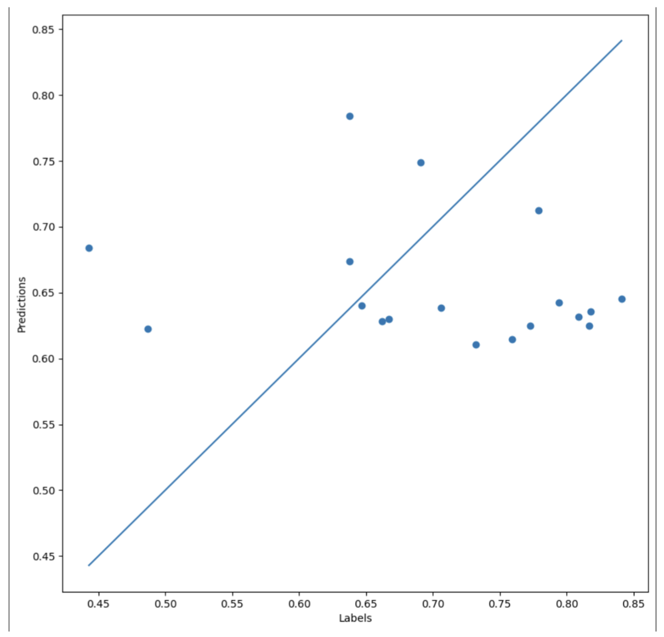
Focusing on the R² scores, although the losses may be low, the R² scores being negative signifies that the model is not able to perform better than a baseline model predicting the mean of each feature. The further negative the R² value is, the more poorly it performs compared to a baseline model. Based on the results for the single output models, valence has the lowest R² score of -0.120 while danceability has the highest R² score of -0.00156. Since this value is closer to 0, it performs almost the same as a baseline model. For reference, the scatter plot representation of the danceability model is included in Figure 4.

Figure 4 is a scatter plot with the labels or actual values on the x-axis and the model’s predictions on the y-axis. Each dot on the plot represents the model’s prediction and how accurate it was. The straight diagonal line represents perfect predictions and accuracy (R² score of 1), so the closer these points are to the line, the higher generalizability of the model. The danceability model had an R² score near 0 and an R² score of 0 would mean that the predictions formed a straight, horizontal line with no clear pattern.

For the multioutput model, the test loss was a combined average of each individual prediction and was higher than the single output model losses with a loss of 0.0385. Its R² score was also the furthest negative from 0 (-0.2558). This demonstrates that when sharing parameters among outputs, it is harder to generalize or predict consistently.

The models were able to optimize and lower training, validation, and test loss but R² values were all negative regardless of target feature or number of outputs. Further detail regarding the results and their implications is mentioned in the Discussion section.

Genre Predictor Results

Model	F1-Score	Accuracy	Precision	Recall
Multi-Layer Neural Network	0.13	28.62%	0.08	0.29
Random Forest	0.36	33.79%	0.47	0.34
Multi-Class Multi-Layer Neural Network	0.39	22.07%	0.34	0.45
Multi-Class Random Forest	0.60	24.48%	0.60	0.66

There were four models being compared on the unseen data, two key architectures one neural network versus another random forest and those architectures were altered for multiclass prediction in which they predict multiple possible genres for a single song. Based on simultaneous inputs the output would be different probabilities for pop (0), hip hop (1), r&b (2), dance/electronic (3), and rock (4). For each model, the F₁-score, accuracy, precision, and recall values were obtained. Precision measures the ratio of true positives out of all the predicted positives while recall measures the ratio of true positives out of all of the actual positives. Higher precision means there would be less false positives or songs predicted to be a certain genre when they are not. On the other hand, higher recall means there would be less false negatives or songs predicted to be another genre when in reality they are the genre that the model is predicting for. Accuracy is the number of correct out of the total predictions and the F₁-score is the harmonic mean of precision and recall, taking both of these into account. For the multi-class versions, accuracy was exact match accuracy for all possible genres.

Accuracy values remained consistently low across each model ranging from 22.07% to 33.79%. Since there are five genres, a random-guess baseline accuracy would be around 20% accuracy and each model did perform better than this statistical reference value. However, they are only higher by a slight margin which means that statistically meaningful genre classification is difficult to achieve through numerical features alone and the inclusion of more semantic features would be necessary.  The multi-class random forest model achieved the highest F₁-score of 0.6 and the highest recall of 0.66, indicating stronger sensitivity to identifying classes, though its accuracy remained low with 24.48%. The standard random forest model reached the highest accuracy of 33.79%  with an F₁-score of 0.36, while the two neural network models performed worse overall in each value compared to the random forests. The basic multilayer neural network produced the lowest F₁-score of 0.13 and precision of 0.08 which is significantly lower than the others but showed a relatively higher recall of 0.29 compared to its precision. This meant it dealt with false negatives better. The multi-class neural network achieved slightly better balance, with an F₁-score of 0.39 and recall of 0.45, but still underperformed relative to the decision tree-based approaches.

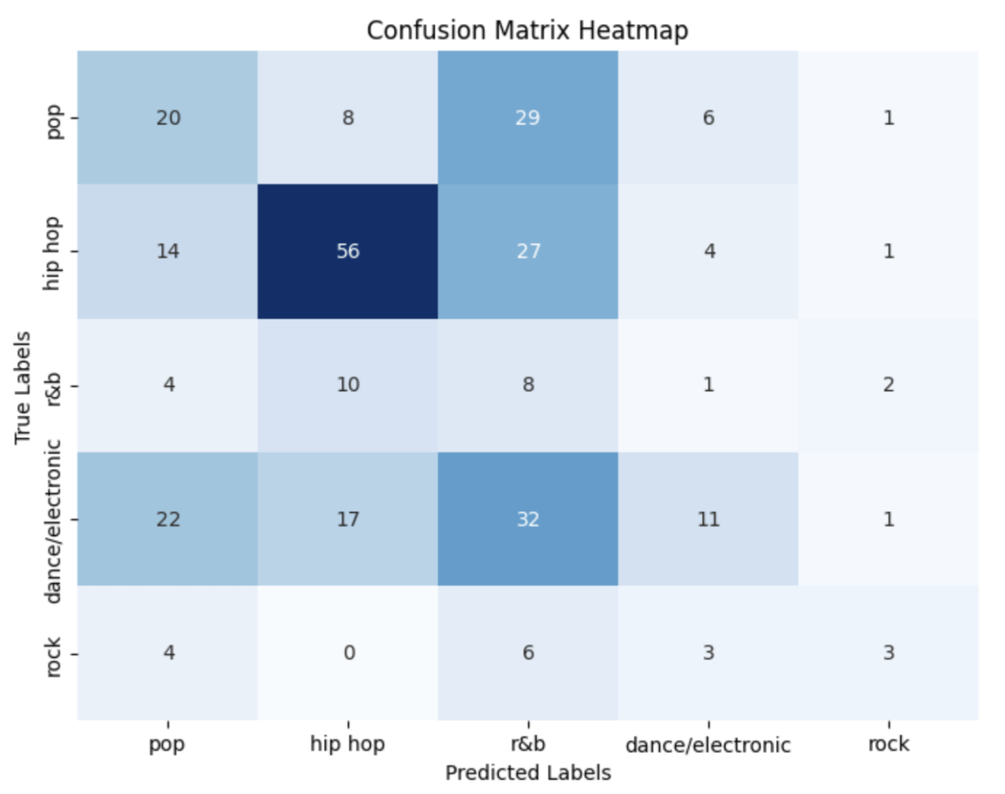
The genre-prediction heat map from the standard random forest’s test (Figure 5) revealed substantial confusion among classes, particularly between pop, R&B, and hip-hop. Hip-hop displayed slightly stronger predictions with most of them being accurate, while rock exhibited inconsistent classification patterns with it being closely followed by dance/electronic as rarely predicted.

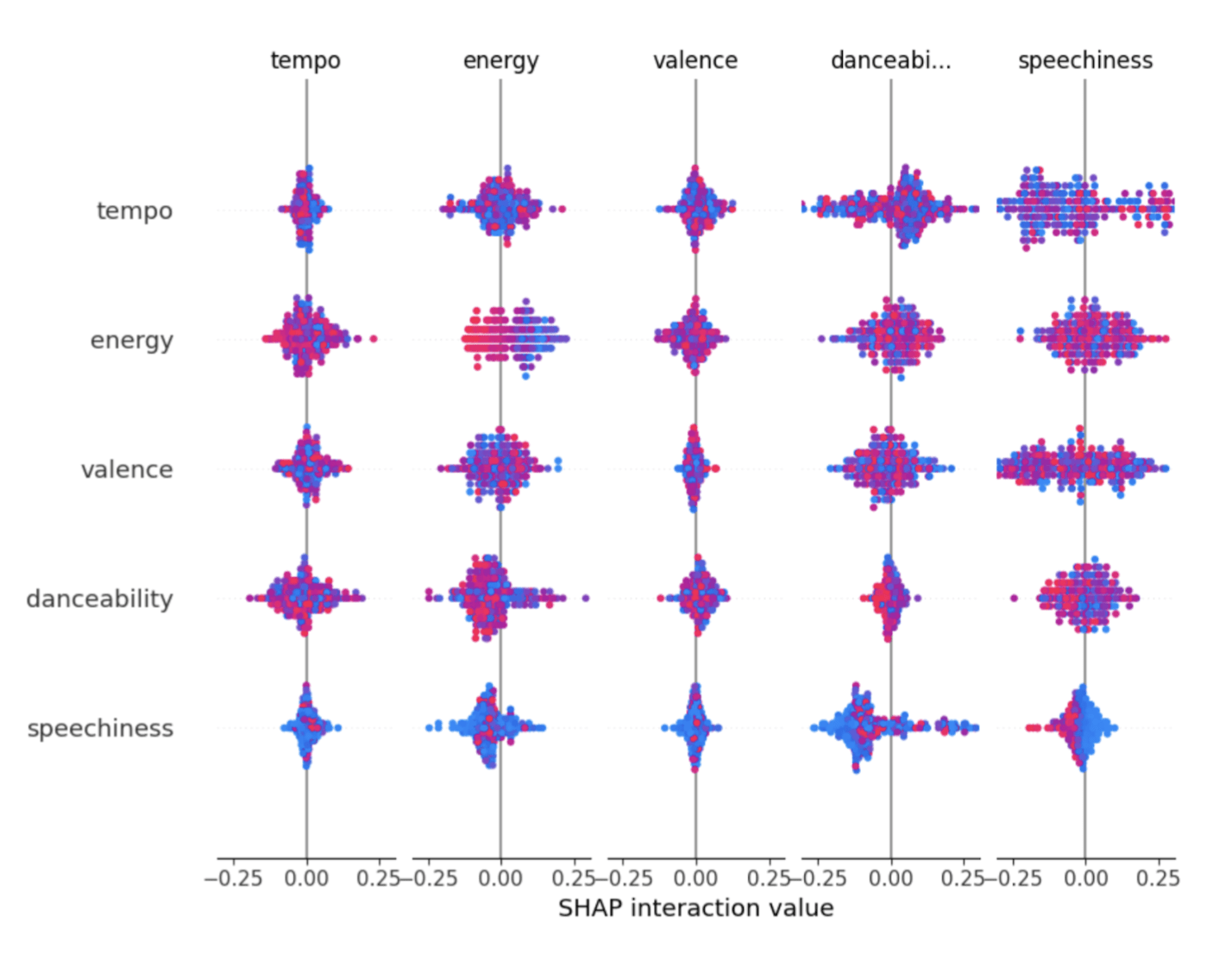
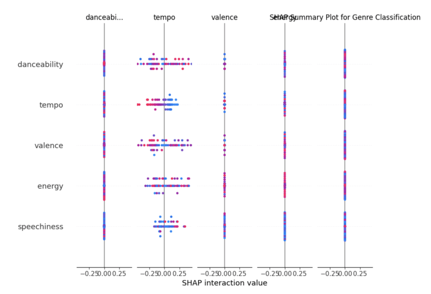
SHAP values for the random forest (Figure 6) highlighted non-linear feature interactions and showed that danceability, speechiness, energy, and valence were consistently interacting with the largest spreads. In contrast, SHAP explanations for the neural network (Figure 7)  revealed less information only showing interactions with tempo and nothing else. These differences suggest that tree-based models were more consistent in learning feature–genre relationships compared to neural networks under the same input constraints and that the neural network was unable to leverage feature interactions in its separation of genres.

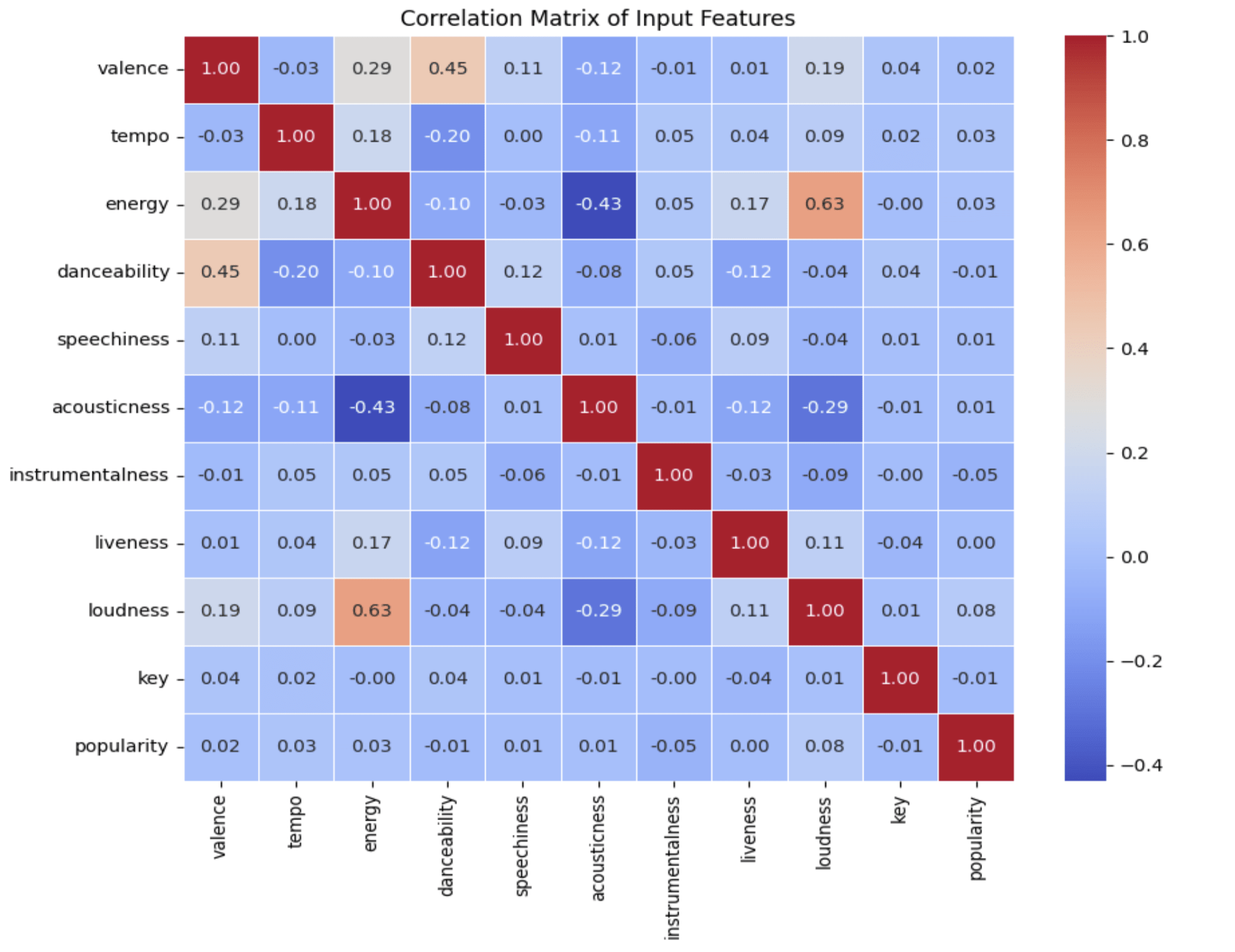
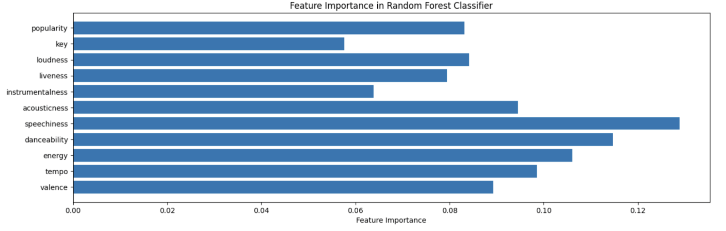
The feature correlation matrix (Figure 8) showed modest relationships among numerical predictors, with no single feature strongly dominating the structure of the dataset. Energy and loudness seem to have similar relationships while valence and danceability are also similar. Energy and acousticness have an inverse relationship.Feature dependence bar graphs for the random forest model (Figure 9) indicated that speechiness, energy-related features, and danceability contributed most to model decisions just like the SHAP plots.While many of the important features are closely congested, there are a few outliers such as popularity and key that serve very little importance for decision-making.

Discussion

In the experiments above, several interesting outcomes were noted:

Overview

1. The feature models tended to perform very well on test data whose true values fell within specific ranges. There was most likely a common range in which most songs used feature values from. Songs of vastly different styles were therefore outliers. For example, it is very uncommon for songs to have tempos below a certain bpm because it is unappealing to the listeners. Therefore, most artists use similar tempos and is why the model picked up on this pattern that a song’s feature values usually fell within a certain range.
2. R² scores were consistently negative highlighting the regression network’s poor generalizability despite low test losses. Figure 4 demonstrates this with the points clustered around a narrow range rather than near the line.
3. The model was unable to capture necessary information to predict the feature simply based on waveform tensors.
4. Between features, not much difference loss wise (energy had 0.0254 while tempo had 0.0298) suggesting that the model was not truly understanding the underlying patterns for each feature (simply taking input for convolution and then spitting out outputs without learning patterns)
5. Accuracies ranged from 22-34% and F₁-scores ranged from 0.13-0.60 (large variety suggesting some models could definitely be improved upon)
6. Random forest models performed much better than the neural network architecture modified from the regression task. 
7. The confusion matrix heatmap (Figure 5) shows significant overlap between categories, particularly among pop, R&B, and dance/electronic. Hip-hop had the most concentration within its diagonal while rock displayed inconsistent classification.
8. The correlation matrix (Figure 8) indicates that most features have weak or moderate correlation with one another ( energy x loudness = 0.63, valence x danceability = 0.45), suggesting limited ability of individual features to drive genre separation.
9. Speechiness, danceability, and energy repeatedly mentioned as primary features for prediction as shown in feature dependence bar graph (Figure 9). Since there was an even distribution in the feature reliance, it can be inferred that a combination of multiple features suggests one genre over another.
10. SHAP plots for neural networks revealed barely any dependence on features other than tempo (even this was weak) while the random forest depended on many of the features in tandem indicating somewhat stable relationships.

Limitations

1. Regression models were not able to predict well on outliers that didn’t fall within the range. Therefore, a more diverse dataset and a greater prevention of  overfitting could prevent the models from incorrectly predicting on outliers.
2. Inability to generalize and predict features shows weakness in waveform patterns. More high-level forms of music information retrieval is preferable. Potential underfitting and inability to map waveform to feature consistently within convolutional regression network. Possibly would have worked better with a transformer architecture or complete CNN rather than tensor-reduced waveforms with linear layers.
3. Genres like pop, hip hop, and r&b have overlap within the features which makes sense as to why the heat map was dense at the top left. There may be other features such as timbre which have greater effect on genre prediction which were not included in the original dataset.
4. The model may have a difficult time predicting since it is only given numerical values, no idea of spatial/temporal structure. Different methods of audio signal processing or deep learning (could potentially strengthen SHAP interactions consistency)  are necessary with larger/more diverse datasets. 
5. Overfitting, potentially due to insufficient variety in training data or other causes, which may have been caused by the multi-label nature of the data or the fact that the dataset was only of popular song could have led to a lack of generalizability

Conclusion

In this paper the feasibility of utilizing waveform information to predict numerical song features is tested as well as how difficult it is to predict genre when given these numerical features. While the regression analysis demonstrated low losses, they were unable to generalize as characterized by their negative R² scores which reflects the difficulty to predict interpretive features such as valence or danceability. These features cannot be simply captured by waveform amplitudes unless audio representation is more rounded, containing more details about an audio track.

The genre classification task exhibited similar issues with five-class classification being difficult when given the numerical audio features. The multi-class random forest model, while being the best performing, was only able to achieve somewhat decent F₁-scores and still had confusion among classes as depicted in the confusion matrix. Correlation, SHAP, and feature analyses proved that the numerical features had weak albeit present discrimination or interaction. Finally, the neural network architectures consistently demonstrated poor and chaotic results without making use of patterns at all. 

Overall, the study suggests that the input feature space led to poor results from both tasks. Spectrograms, MFCCs and possibly other architectures remain strong in regression tasks related to audio-based deep learning. Although model robustness could be enhanced it is still clear that genre classification should be approached in a different manner and waveforms are not strong enough contenders to effectively perform audio-based deep learning tasks. The results underscore the significance of choosing appropriate feature representations when working with complex music phenomena and would be a much stronger foundation for more advanced audio-based predictive systems.

Acknowledgements

I would like to thank Mariel Werner from UC Berkeley for guiding me through creating the machine learning model and providing feedback during the experimentation and the writing of this paper.

Appendix

Link to code created for project: https://colab.research.google.com/drive/1UTVEkKl7dkaYHtWEd5ZJ2Xyrk5DAfStp?usp=sharing

References

1. Vanessa Van Edwards. (2019, July 29). The Benefits of Music: How the Science of Music Can Help… Science of People; Science of People. https://www.scienceofpeople.com/benefits-music/. [↩]
2. Léonard, F. (2007). Phase spectrogram and frequency spectrogram as new diagnostic tools. Mechanical Systems and Signal Processing, 21(1), 125–137. https://doi.org/10.1016/j.ymssp.2005.08.011. [↩]
3. Zhang, J. (2021). Music Feature Extraction and Classification Algorithm Based on Deep Learning. Scientific Programming, 2021, 1–9. https://doi.org/10.1155/2021/1651560. [↩]
4. Kaminskas, M., & Ricci, F. (2012). Contextual music information retrieval and recommendation: State of the art and challenges. Computer Science Review, 6(2-3). https://doi.org/10.1016/j.cosrev.2012.04.002. [↩] [↩]
5. Mitrović, D., Zeppelzauer, M., & Breiteneder, C. (2010). Features for Content-Based Audio Retrieval. Advances in Computers, 71–150. https://doi.org/10.1016/s0065-2458(10)78003-7. [↩] [↩]
6. Rao, P. (2007). Audio Signal Processing. In Studies in Computational Intelligence (Vol. 83, pp. 169–189). https://doi.org/10.1007/9783540753988_8. [↩]
7. Picken, J. (2023, September 21). Music Genres Explained | Blog | Startle Music. Www.startlemusic.com. https://www.startlemusic.com/blog/music-genres-explained. [↩]
8. Bahuleyan, H. (2018). Music Genre Classification using Machine Learning Techniques. https://arxiv.org/pdf/1804.01149. [↩]
9. Corrêa, D. C., & Rodrigues, F. Ap. (2016). A survey on symbolic data-based music genre classification. Expert Systems With Applications, 60, 190–210. https://doi.org/10.1016/J.ESWA.2016.04.008. [↩]
10. Henrique, P. (2021, January 31). Predicting Music Genres Using Waveform Features | Towards Data Science. Towards Data Science. https://towardsdatascience.com/predicting-music-genres-using-waveform-features-5080e788eb64/. [↩]
11. AltexSoft. (2022, May 12). Audio Analysis With Machine Learning: Building AI-Fueled Sound Detection App. AltexSoft. https://www.altexsoft.com/blog/audio-analysis/. [↩]
12. Katsiaryna Ruksha. (2024, January 19). Music Information Retrieval: Introduction – Katsiaryna Ruksha – Medium. Medium; Medium. https://medium.com/@kate.ruksha/introduction-into-music-information-retrieval-part-1-2dc874cda763. [↩]
13. Wim van Drongelen. (2007). Continuous, Discrete, and Fast Fourier Transform. Elsevier EBooks, 91–105. https://doi.org/10.1016/b978-012370867-0/50006-1. [↩]
14. Doshi, K. (2021, February 11). Audio Deep Learning Made Simple (Part 1): State-of-the-Art Techniques | Towards Data Science. Towards Data Science. https://towardsdatascience.com/audio-deep-learning-made-simple-part-1-state-of-the-art-techniques-da1d3dff2504/. [↩] [↩]
15. Van Den Oord, A., Dieleman, S., Zen, H., Simonyan, K., Vinyals, O., Graves, A., Kalchbrenner, N., Senior, A., & Kavukcuoglu, K. (2016). WAVENET: A GENERATIVE MODEL FOR RAW AUDIO. arXiv. https://arxiv.org/pdf/1609.03499. [↩]
16. Koverha, M. (2022, May 31). Top Hits Spotify from 2000-2019. Www.kaggle.com. https://www.kaggle.com/datasets/paradisejoy/top-hits-spotify-from-20002019. [↩]
17. Sai Kanuri, V. (2022, October 12). Spotify Data Visualization. Kaggle.com. https://www.kaggle.com/code/varunsaikanuri/spotify-data-visualization. [↩]
18. muzammilbaloch. (2024, March 25). Spotify Hits Analysis and Prediction🎶📊. Kaggle.com; Kaggle. https://www.kaggle.com/code/muzammilbaloch/spotify-hits-analysis-and-prediction. [↩]
19. Rangwala, B. (2021, July 23). Audio Classification and Regression using Pytorch – Burhanuddin Rangwala – Medium. Medium; Medium. https://bamblebam.medium.com/audio-classification-and-regression-using-pytorch-48db77b3a5ec. [↩]
20. Pykes, K. (2024, January 11). Cross-Entropy Loss Function in Machine Learning: Enhancing Model Accuracy. Datacamp.com; DataCamp. https://www.datacamp.com/tutorial/the-cross-entropy-loss-function-in-machine-learning. [↩]
21. Pytorch. (2023). CrossEntropyLoss — PyTorch 1.6.0 documentation. Pytorch.org. https://pytorch.org/docs/stable/generated/torch.nn.CrossEntropyLoss.html [↩]