Stock Closing Price Prediction Using Kinetic Energy and Stochastic Processes

Binh Ho, Tran Minh Nghia, Anh Nguyen, Vi Nguyen & Tung Ngo

January 19, 2026

141

Abstract

In recent years, there has been a growth in the use of algorithms and machine learning models in stock price prediction. This research paper studied the change of the S&P 500 index from December 6, 2023, to December 2, 2024. A forecasting model was developed based on the idea of kinetic energy to predict the value of stock closing price of the S&P 500 companies. The proposed model treats price changes and trading volume as analogues to velocity and mass, respectively, allowing stock dynamics to be represented through a kinetic energy formulation. The model’s performance is evaluated against that of the other benchmark models – ARIMA(p,d,q), Double Exponential Smoothing, and Artificial Neural Network – in terms of mean absolute error (MAE) and mean absolute percentage error (MAPE). The models were then backtested for evaluation on mean returns, and Sharpe Ratio. In predicting the future prices after the last date of the training set of the S&P 500 stocks, the Kinetic Energy-based model generated more accurate price predictions for short-term forecasting than other benchmark models. Furthermore, the results of the mean returns and Sharpe Ratio showed that while the Kinetic Energy-based model is better suited for generating returns, its Sharpe Ratio indicates that these returns exhibit higher volatility than those of some benchmark models. Overall, the Kinetic Energy-based model demonstrates a strong potential for short-term prediction, though its return stability remains a limitation.

Introduction

Background

The stock markets are defined as locations for economic transactions of buying and selling stocks, which are the financial ownership claims of businesses. Throughout history, the stock market has played a crucial role in the advancement of the economy and emerging markets¹ . One way businesses influence the change in stock prices is through the process of buying and selling stock, which causes the stock prices to fluctuate over time in a dynamic, unpredictable, and non-linear nature² . Other ways are through external factors such as political conditions, financial articles, and social media. For these reasons, predicting a stock price in advance to maximize a trading strategy is a challenging process. There are two main methods for predicting the future value of a stock price: quantitative and qualitative techniques² . For the quantitative method, researchers employ statistical models that predict the stock price using historical data of the stock price, such as the opening and closing prices, the traded volume, and the daily low and high prices. For the qualitative method, researchers develop models that take into account the external factors discussed above. This paper focuses more on the quantitative side of stock price forecasting.

Research gap and problem statement

In Physics, there is a concept known as Kinetic Energy (KE) that describes the energy of a system of particles or objects with movement. KE relates the mass of an object with its velocity. The formula for KE is described below, where ”m” is the mass of a body under some velocity ”v”. Usually, ”m” is measured in kilograms (kg) and ”v” is measured in meter per second (m/s)³. Given the mass m and velocity v of a particle or object, its Kinetic Energy (KE) is defined as³

(1) $\begin{equation*}KE = \frac{1}{2}mv^2\end{equation*}$

In a research paper by Kiyoshi Kanazawa et al.⁴ on the relationship between kinetic theory and finance Brownian motion, the authors argue that the financial markets resemble the hierarchical structure of the conventional Brownian motion. The authors claim that one can imagine those hierarchies directly correspond to those in the kinetic theory: traders, order books, and price correspond to molecules, velocity distribution, and Brownian particles, respectively. From these similar characteristics between components in kinetic theory and financial markets, some researchers aim to study the stock market with the assistance of the concepts in kinetic theory, particularly, the kinetic energy. In another research paper by Morteza Zahedi and Mahdieh Ghotbi⁵ , the authors exploited the idea of kinetic energy to examine features of financial market, aiming to provide more accurate predictions of stock prices. The authors proposed the three approaches: RSIK, DRLK, and TDQNK. More specifically, the RSIK combined kinetic energy with the traditional RSI to predict the signal of the market; if the signal is -1 and kinetic energy is greater than the predetermined threshold, the authors claim the predicted signal to be sold. The DRLK incorporates kinetic energy to the traditional DRL model, operating anti-signal action on the trading environment. The TDQNK integrates the TDQNK, a deep reinforcement learning model, and kinetic energy, and uses the Huber loss for the training process.

In analyzing GBPUSD, the RSIK outperformed the RSI and other traditional strategies at 0.95 average measures. Likewise, in analyzing XAUUSD, the RSIK outperformed the RSI and other traditional strategies at 0.48 average measures. In analyzing APPL and XAUUSD, the DRLK outperformed DL at 22.16 and 7.35, respectively. Finally, the TDQNK outperformed the TDQN as a trading strategy, gaining a profit of 116216 and an annualized return of 35.75 %. The argument from Kiyoshi Kanazawa et al.⁴ and the results from Morteza Zahedi and Mahdieh Ghotbi⁵ show that kinetic energy can be applied in stock price prediction and trading strategy to gain advantage over other traditional models and techniques. Such a relationship led us to study the ability to predict stock prices based on kinetic energy.

Objectives

The objectives of this paper are to analyze the change in the S&P 500 index, develop a model that predicts the individual stock closing prices using the idea of kinetic energy, and evaluate the model against other widely known forecasting models.

This study focuses on answering the following guiding questions:

How did the S&P 500 index change from December 4, 2023 to December 2, 2024?
What is the relationship between the individual stock closing prices and kinetic energy in our model?
How does our model compare to other existing models in the literature?

We hypothesized that it is possible to predict stock closing prices with the concept of kinetic energy, and that the Kinetic Energy-based model would have some advantages over other traditional forecasting models.

Literature review

Autoregressive Integrated Moving Average Models

One of the most common traditional model for time-series forecasting, such as stock price prediction, is the Autoregressive Integrated Moving Average, also known for short as ARIMA(p,d,q). A research study by Sidharth Tiwary and Pramod K. Mishra⁶ used ARIMA (p,d,q) as a basis for their prediction of stock prices. The study utilized the data on TESLA and NIO stock details from December 10, 2018 to June 3, 2022 and fit the ARIMA(p,d,q) according to the Box and Jenkins Methodology.

Definition 2.1⁶ According to the ARIMA(p,d,q) model, the stock closing price is the linear combination of its lagged values and lagged errors. That is

(2) $\begin{align*}y_t = c + \phi_1 y_{t-1} + \phi_2 y_{t-2} + \dots + \phi_p y_{t-p} + \epsilon_t \\- \theta_1 e_{t-1} - \theta_2 e_{t-2} - \dots - \theta_q e_{t-q}\end{align*}$

where,

$y_t$ : Stock closing price at time $t$
$c$ : Constant term (intercept)
$\phi_1, \phi_2, \dots, \phi_p$ : Autoregressive (AR) coefficients
$y_{t-1}, y_{t-2}, \dots, y_{t-p}$ : Lagged closing price values
$\epsilon_t$ : White noise at time $t$
$\theta_1, \theta_2, \dots, \theta_q$ : Moving Average (MA) coefficients
$e_{t-1}, e_{t-2}, \dots, e_{t-q}$ : Lagged error terms

Using Auto-ARIMA, an algorithm to find the optimal parameters ”p,d,q”, the study obtained ARIMA(0,1,0) as the best ARIMA model for the closing price of TESLA and ARIMA (1,1,1) as the best ARIMA (p,d,q) model for that of NIO. Forecasting with a confidence level 95% for the next 15 days after the training set, the models for the TESLA and NIO stock price prediction resulted in mean absolute percentage errors (MAPEs) of 0.03% and 0.18%, respectively. Although the errors were considerably low, the ARIMA (p,d,q) model has some drawbacks. Firstly, it only relies on the linear relationship between the lagged variables and between the moving averages. Such linear assumptions lead to the model disadvantage when dealing with non-linear relationships. Secondly, as explained in the research paper by Sidharth Tiwary and Pramod K. Mishra⁶ , the ARIMA (p,d,q) model requires the data to be stationary, meaning its statistical properties – such as mean and variance – stay constant over time, which might not be the case in the real stock market, where there are trends to the prices. These disadvantages led us to research and develop an alternative forecasting model that does not rely on the linear and stationary assumptions. The models that utilize concepts in kinetic theory, according to Kiyoshi Kanazawa et al.⁴ and Morteza Zahedi and Mahdieh Ghotbi⁵ , do not assume linear relationships between time series lagged values and stationarity of the time series itself, thus mitigating the discussed drawbacks that the ARIMA (p,d,q) model has.

Double Exponential Smoothing Model

Other traditional models that are widely exploited in time series forecasting of stock price are Exponential Smoothing (ES) techniques. An ES model that we employed in this study is the Double Exponential Smoothing model, which has an advantage over other types of ES models – such as the Simple Exponential Smoothing model – in predicting time series that have trends. A research study by Aminur Rahmanon⁷ the predictability of ES models in stock price prediction discussed the use of the Double Exponential Smoothing model.

Definition 2.2⁷According to the Double Exponential Smoothing model, the stock price at time t is the summation of the weighted average level and trend at time t-1.

That is

(3) $\begin{align*}L_t &= \alpha V_{STK_t} + (1 - \alpha)(L_{t-1} + T_{t-1}) \\T_t &= \theta(L_t - L_{t-1}) + (1 - \theta)T_{t-1} \\\hat{V}{STK_t} &= L{t-1} + T_{t-1}\end{align*}$

where,

$L_t$ : the level at time $t$
$\alpha$ : the weight for the level
$T_t$ : the trend at time $t$
$\theta$ : the weight for the trend
$V_{STK_t}$ : the stock price at time $t$
$\hat{V}_{STK_t}$ : the predicted price at time $t$

The data of weekly stock prices of Pearson PLC (PSON.L), Burberry Group PLC (BRBY.L), JD plc (JD.L), Access Intelligence plc (ACC.L), and Aptitude Software Group plc (APTD.L) from May 31, 2009 to February 11, 2024 is fit to the model. The forecast period is not explicitly discussed in this study.

The results show that the MAPEs for the Double Exponential Smoothing when forecasted for those companies are 1.33%, 4.3%, 31.07%, 3.18%, 18.22%, respectively. One reason that we decided not to study the Triple Exponential Smoothing model (also known as the Holt-Winters model) was because the study above shows that it has an inferior performance to the Double Exponential Smoothing in terms of MAPEs⁷ . Although the Double Exponential Smoothing model performs considerably well in the context of the above study, displaying some low MAPEs, the model has a disadvantage. The model assumes that the trend of the time series in the past will persist in the future, which is problematic if the trend in the stock prices changes. This problem led us to research and develop an alternative forecasting model that does not rely heavily on the time series’ trend.

Artificial Neural Network

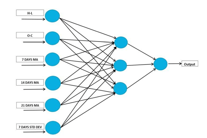
Besides traditional models, there are other widely known methods for time-series forecasting, such as stock price prediction, that incorporate machine learning techniques. A research study by Mehar Vijh et al.² used artifical neural network (ANN), fitted from April 6 2009 to April 3 2017, to predict closing stock price of Nike, Goldman Sachs, Johnson and Johnson, Pfizer and JP Morgan Chase and Co from April 4, 2017 to April 5, 2019. The study claims that the input nodes for the ANN model were the difference of High and Low price, the difference of Close and Open price, stock price’s seven days’, fourteen days’, and twenty one days’ moving average, and stock price’s standard deviation for the past seven days. The weights of each input node are multiplied and sent to the neurons in the hidden layer, and the output layer consists of only one neuron, which gives the predicted closing price.

The results show that the ANN’s MAPEs for the closing price of Nike, Goldman Sachs, Johnson and Johnson, Pfizer and JP Morgan Chase, and Co were 1.07%, 1.09%, 0.89%, 0.70%, 0.77%, respectively. Despite having pronounced results, the ANN model possesses one main challenge. Since the ANN model has hyperparameters such as the number of hidden layers, learning rate, and activation function, the model should be hyperparameter tuned before training to enhance the performance, which can be computationally costly. Therefore, it led us to research and develop an alternative forecasting model that minimizes the drawbacks of hyperparameter tuning.

Neural networks contain several hyperparameters, such as the number of hidden layers, activation functions, learning rate, and batch size, which affect how well the model learns. Without tuning these hyperparameters, the network can easily overfit the training data and perform poorly on unseen prices. More advanced architectures, such as Long Short-Term Memory (LSTM) networks, can model long-term price behavior, but they require larger datasets, a greater number of parameters, and longer training time. Since our goal was to compare our kinetic-energy-based approach to commonly used baseline models while keeping computation accessible, we chose to implement the ANN model instead of the LSTM in this study.

Methodology

Data collection and preprocessing for models comparison

To implement the forecasting models, we collected the data about the stock closing prices of the S&P 500 companies. The datasets were gathered using the finance library⁸ , a website that provides real-time financial information and stock market data. The datasets were from December 4, 2023 to December 2, 2024, a period of about one year. We decided to test our model against the ARIMA(p,d,q), Double Exponential Smoothing, and the ANN models, which were the ones discussed in section 2. For each of these models, we split the dataset into training and test sets, where training sets were the first 80% of the data and test sets were the remaining 20%. Therefore, the training sets were from December 6, 2023 to September 19, 2024, and the test sets were from September 20, 2024 to December 2, 2024. To avoid any null values, we drop any data points with NaN values

To implement the ARIMA(p,d,q) model, we first tested for the stationarity of the datasets for those companies because stationarity is an assumption of any ARIMA(p,d,q) model⁹ . To do so, we employed the Augmented Dickey-Fuller (ADF) test¹⁰ on the training sets. The null hypothesis (H₀) of the ADF test is that the series is nonstationary, and the alternative hypothesis (H₁) is that the series is stationary. An ADF test which results in a p-value< α rejects the H₀, suggesting that the series is stationary. For this study, we chose 0.05 as the value for α (significant level) because it is one of the most common values for a significance level¹¹ . Table 1 shows the results for the ADF test on the original training sets of the S&P 500 stocks.

Original Series	ADF test p-value
A	0.041
AAPL	0.911
ABBV	0.541
	…
ZBH	0.713
ZBRA	0.697
ZTS	0.545

Table 1 | ADF test results for the original training datasets¹²

The results from Table 1 show that some of the training sets for the original series of the companies are not stationary with p-values greater than α = 0.05. While some are stationary with p-values less than α = 0.05. Therefore, we decided to differentiate the original series and run the ADF test again. The definitions were formed to assist in this process.

Definition 3.1 Since the closing stock price is recorded daily in our datasets, its timesteps are recorded discretely and evenly spaced. A time series of a stock closing price P is defined as an ordered sequence of stock closing prices at the allowed discrete time-step t ∈ T = {0,1,2,3,..,n}, where n is the last date in the series. That is

(4) $\begin{equation*}P = (P(0), P(1), P(2), P(3), \dots, P(n)) = {P(t)}_{t=0}^n\end{equation*}$

Definition 3.2 From Definition 3.1, the first order differenced series is defined as

(5) $\begin{align*}P' &= \left(\frac{P(1) - P(0)}{t_1 - t_0}, \frac{P(2) - P(1)}{t_2 - t_1}, \dots, \frac{P(n) - P(n-1)}{t_n - t_{n-1}}\right) \\&= \left(\frac{P(1) - P(0)}{1}, \frac{P(2) - P(1)}{1}, \dots, \frac{P(n) - P(n-1)}{1}\right) \\&= {P(t) - P(t-1)}_{t=1}^n\end{align*}$

From Definition 3.2, we ran the ADF test on the first ordered differenced training datasets. The results from Table 2 show that the first order differenced training series for all companies but SW are stationary because all p-values are less than $\alpha = 0.05$ except for SW with a p-value of $0.07 > 0.05$ . After the second order differentiation, the p-value for SW is $3.708 \times 10^{-09} < 0.05$ , indicating stationarity.

First Order Differenced Series	ADF test p-value
A	6.591 ∗ 10⁻¹⁴
AAPL	1.974 ∗ 10⁻²³
ABBV	5.162 ∗ 10⁻²⁶
…
ZBH	1.021 ∗ 10⁻²⁷
ZBRA	2.147 ∗ 10⁻²⁵
ZTS	1.537 ∗ 10⁻¹⁹

Table 2 | ADF test results for the first order differenced training datasets¹³

To find the optimal values for the parameters p,d,and q in the ARIMA(p,d,q) models, we employed the Auto-ARIMA¹⁴ , an algorithm that calculates such optimal parameters, to the training series of the three companies. Table 3 shows the optimal parameters for the ARIMA(p,d,q) models of the series.

Series	Optimal parameters for ARIMA(p,d,q)
A	ARIMA(3,0,0)
AAPL	ARIMA(0,1,0)
ABBV	ARIMA(0,1,0)
	…
ZBH	ARIMA(0,1,0)
ZBRA	ARIMA(0,1,0)
ZTS	ARIMA(0,1,0)

Table 3 | The optimal parameters for the ARIMA(p,d,q) for the training datasets¹⁵

The Double Exponential Smoothing models do not require as many preprocessing steps. We utilized the framework introduced in Definition 2.2. We then performed an optimization process to find the optimal weights for the level ( $\alpha$ ) and the trend ( $\theta$ ) of the S&P 500 training series that minimize the error of the loss function. That is,

(6) $\begin{align*}\alpha &= \min_{\alpha} \sum_{t=0}^n (L_{t-1} + T_{t-1} - P_t)^2 \\theta &= \min_{\theta} \sum_{t=0}^n (L_{t-1} + T_{t-1} - P_t)^2\end{align*}$

where,

$L_{t-1}$ : the forecasted level one time step before time $t$
$T_{t-1}$ : the forecasted trend one time step before time $t$
$P_t$ : the stock closing price at time $t$

Table 4 shows the optimal value of α and θ for the training series.

Series	Optimal α	Optimal θ
A	0.100	0.031
AAPL	0.100	0.099
ABBV	0.100	6.33 ∗ 10⁻¹¹
	…
ZBH	0.942	0.051
ZBRA	0.100	0.054
ZTS	0.100	0.056

Table 4 | The optimal parameters for the Double Exponential Smoothing for the training datasets¹⁶

To implement the ANN model, we followed the architecture introduced in section 2.3² to let the model have six input neurons:

Stock High minus Low price (H-L).
Stock Close minus Open price (O-C).
Stock price’s seven days’ moving average (7 DAYS MA).
Stock price’s fourteen days’ moving average (14 DAYS MA).
Stock price’s twenty one days’ moving average (21 DAYS MA).
Stock price’s standard deviation for the past seven days (7 DAYS STD DEV).

In the study² in the literature, the authors utilized the ANN architecture with three hidden neurons and one single output neuron for the value of the closing price. Refer to Figure 1 for the detailed architecture. However, we acknowledged that the optimal architecture of that study might not be the optimal architecture when applied in our study. We decided to implement a method of hyperparameter tuning called Random Search, which computes the optimal hidden layer size, activation, learning rate, and batch size from a search space for the ANN model. However, tuning such hyperparameters for every individual S&P 500 stocks is computationally costly so we decided to combine all tickers into one dataset and pass it through the Keras Tuner’s Random Search function¹⁷ . To speed up the search, we used a random subset of up to 5000 samples from the training data. Table 5 shows the optimal hyperparameters for the ANN model after tuning. Note that we kept the input layer to have six input neurons as in the study in section 2.3².

Hidden units (layer 1)	Activation (layer 1)	Hidden units (layer 2)	Activation (layer 2)	Learning rate	Batch size
4	tanh	8	ReLu	0.00218	32

Table 5 | The optimal hyperparameters for the ANN model.

Figure 1 | The detailed architecture of the ANN models used in the literature

For backpropagation, we used the algorithm Adam, an adaptive gradient descent algorithm and a widely used stochastic optimizer¹⁸ .

To implement the three models as well as our proposed one, we first normalize the data for the closing prices of the S&P 500 stocks to avoid any outliers and redundancies, leading to better model performance. The normalization technique we used in this study was the log-transformation, following Definition 3.3.

Definition 3.3 Given a data point X_i, its log-transform value is computed as Y_i where

(7) $\begin{equation*}Y_i = \log(X_i + (1 - \min(X)))\end{equation*}$

We then applied the log-transform to the input data to train and test the performance of the ARIMA(p,d,q), Double Exponential Smoothing, ANN, and our proposed model (Kinetic Energy-based model). Since the outputs of the models, which are the closing prices, are continuous, we also normalize the outputs for training and testing.

Forecasting model with Kinetic Energy formulation

In this section, we will discuss the formulation of our forecasting model for the stock closing using the idea of Kinetic Energy and stochastic processes.

The model is inspired by the formula for KE introduced in section 1.2. Note that the data points are normalized with the log-transform method introduced in Definition 3.3.

Definition 3.4 The formula for the KE of a stock closing price at time t is computed as

(8) $\begin{equation*}KE(t) = \frac{1}{2}m(t)v(t)^2\end{equation*}$

where $m(t)$ is the trading volume at time $t$ and $v(t)$ is the rate of change of the stock closing price or the differenced value of the closing price (introduced in Definition 3.2) at time $t$ . That is

(9) $\begin{equation*}v(t) = P(t) - P(t-1)\end{equation*}$

The reason we chose the “mass” term of the KE formula as the trading volume is due to its relationship with the price. According to a study about the effect of the trading volume on stock price¹⁹ , an increase in the trading volume is associated with an increase in the average stock price. Notice that KE(t) and m(t) are proportional, meaning that an increase in m(t) will lead to an increase in KE(t). Consequently, an increase in KE(t) will likely lead to an increase in its value on the next time step KE(t + 1), leading to an increase in stock closing price P(t + 1) as the result of an increase in v(t + 1).

Definition 3.5 From Definition 3.4, the future stock closing price N time step after can be computed as

(10) $\begin{equation*}\hat{P}(t+N) = v(t+N) + P(t)\end{equation*}$

(11) $\begin{equation*}\hat{P}(t+N) = \pm \sqrt{\frac{2\hat{KE}(t+N)}{\hat{m}(t+N)}} + P(t)\end{equation*}$

Let the term $\pm \sqrt{\frac{2\hat{KE}(t+N)}{\hat{m}(t+N)}}$ be $\hat{v}(t+N)$ . Its sign is chosen based on the empirical probability in the training set. That is, given a random variable $X$ taking on ${-1, +1}$ with the probability of the rate of change of $v$ being positive and negative $P(X=+1) = p$ and $P(X=-1) = 1-p$ , then

(12) $\begin{equation*}\hat{v}(t+N) = X * |v(t+N)|\end{equation*}$

To implement this model, the future KE and trading volume $m$ need to be known beforehand, which is impossible. To estimate $KE(t+N)$ and $m(t+N)$ , we proposed an approach to find such values based on their distribution of change.

Definition 3.6 Given the kinetic energy at time t KE(t), the kinetic energy at time t+N is computed as

(13) $\begin{equation*}\hat{KE}(t+N) = (1 + e_{KE}) * KE(t)\end{equation*}$

where, $e_{KE}$ is a random percent change of KE that follows some distribution of all past percent change of KE in the training series.

Definition 3.7 Given the trading volume at time $t$ $m(t)$ , the trading volume at time $t+N$ is computed as

(14) $\begin{equation*}\hat{m}(t+N) = (1 + c_m) * m(t)\end{equation*}$

where, $e_{KE}$ is a random percent change of $m$ that follows some distribution of all past percent change of $m$ in the training series.

To find $e_{KE}$ and $e_m$ , an approximation technique can be utilized based on the distribution of $e_{KE}$ and $e_m$ . The first approach was to assume normal distribution for $e_{KE}$ and $e_m$ of each series and simulate their values from the normal distribution. However, financial returns exhibit heavy tails and volatility clustering, even when they are log-transformed, so normal distribution can not be assumed. To express this property evidently from the data, we employed the Shapiro-Wilk test for normal distribution, which has the null hypothesis that the distribution is normal and the alternative hypothesis that such a distribution is not normal. Table 6 shows the result for the Shapiro-Wilk test²⁰ for normal distribution of e_KEand e_m. As noticed, some series have p-value less than 0.05 for the distribution of e_KEand e_m, supporting the alternative that the series are not normally distributed. Therefore, the first approach was not applicable.

Series	p-value (e_KE)	p-value (e_m)
A	1.152×10^-18	1.969×10^-8
AAPL	1.00	7.723×10^-9
ABBV	7.816×10^-18	9.189×10^-4
	…
ZBH	2.14×10^-18	5.699×10^-4
ZBRA	1.97×10^-20	9.611×10^-7
ZTS	1.00	1.574×10^-6

Table 6 | Results for the Shapiro-Wilk test on e_KEand e_m of all series

The second approach was to approximate e_KEand e_m by assuming any kind of distribution that they exhibit and simulate their values from that empirical distribution. Definition 3.8 and Definition 3.9 model e_KEand e_m, respectively,using this second approach.

Definition 3.8 According to Definition 3.6 and Theorem 3.1, the KE at time t + N is computed as

(15) $\begin{equation*}\hat{KE}(t+N) = (1 + c_{KE}) * KE(t)\end{equation*}$

where, $e_{KE}$ follows a some distribution from its past values. That is,

(16) $\begin{equation*}e_{KE} \sim Distribution(\mu_{e_{KE}}, \sigma_{e_{KE}})\end{equation*}$

where, $\mu_{e_{KE}}$ is the mean and $\sigma_{e_{KE}}$ is the standard deviation of all $e_{KE}$ .

Definition 3.9 According to Definition 3.7 and Theorem 3.2, the trading volume m at time t + N is computed as

(17) $\begin{equation*}\hat{m}(t+N) = (1 + c_m) * m(t)\end{equation*}$

where, $e_{KE}$ some distribution from its past values. That is,

(18) $\begin{equation*}c_m \sim Distribution(\mu_{e_m}, \sigma_{e_m})\end{equation*}$

where, $\mu_{e_m}$ is the mean and $\sigma_{e_m}$ is the standard deviation of all $e_m$ .

With those formulas and theorems above, we can compute the future stock closing price. However, to avoid misleading results from the random variables $e_{KE}$ and $e_m$ , we decided to employ the Monte Carlo Simulation²¹ . We ran 100 simulations for each new time step. Vector of simulations for the next time steps were obtained. That is, for some new time step k,

$P^{(1)}(t+k){MC} &= [P^{(1)}(t+1), P^{(1)}(t+2), \dots, P^{(1)}(t+k)] \nonumber \ P^{(2)}(t+k){MC} &=$

$[P^{(2)}(t+1), P^{(2)}(t+2), \dots, P^{(2)}(t+k)] &\dots P^{(1000)}(t+k){MC} &=$

(19) $\begin{equation*}[P^{(1000)}(t+1), P^{(1000)}(t+2), \dots, P^{(1000)}(t+k)]\end{equation*}$

where $P^{(i)}(t+k){MC}$ is the i-th vector of from the Monte Carlo simulations. We then average out the simulated vectors to get the estimate of the stock closing price at the future time steps from the Monte Carlo simulations. That is,

(20) $\begin{equation*}\widehat{P(t+k)}{MC} = \frac{1}{100} \sum{i=1}^{100} P^{(i)}(t+k)_{MC}\end{equation*}$

To avoid overfitting from assuming the distribution of $e_{KE}$ and $e_m$ , we employed a regularization technique that weighs the average of the prediction from the Monte Carlo simulations and the mean of the five most recent closing prices ( $\mu_{Precent}$ ). This weighted average prevents the model from overfitting the past’s distribution of $e_{KE}$ and $e_m$ , while preserving the trend from the recent closing prices. The estimation of the stock closing price at the future time steps $k$ is calculated as

(21) $\begin{equation*}\widehat{P(t+k)} = \beta \widehat{P(t+k)}{MC} + (1-\beta) \hat{\mu}{P_{recent}}\end{equation*}$

To find the optimal weight $\beta$ for each series, we minimized the loss function between the predicted and true closing price for each series. That is

(22) $\begin{equation*}\beta^* = \arg \min_{\beta} |\widehat{P(t+k)} - P(t+k)_{true}|\end{equation*}$

Refer to the Appendix for the detailed pseudocode for the Kinetic Energy-based model in predicting future prices at time $t+N$ . For reference, to run the simulations, we utilized Google Colab’s T4 GPU which has the GPU memory of 16 GB and 320 GB per second bandwidth²² . There are a total of 250 time steps for our dataset and 4 variables per step. For each step, there are 2 operations – read and write – with float size of 8 bytes for float64 data type. Then the memory moved per step per path is 6x2x8 = 96 bytes. Since there are 100 simulations for each series, the memory per series is 100x250x96 = 2,400,000 bytes, which is 2.4MB. There are a total of 500 series, so the total memory for all 500 series is 2.4×500 = 1200 MB, which is 1.2 GB. As mentioned, the T4 GPU can move 320 GB per second, so the memory time required to run 100 simulations for 500 series to predict 1 time step in the future is about 1.2/320 = 0.00375 second. Note that the regularization process introduces minimal computational overhead because it only requires the mean of the five most recent closing prices, and it performs a simple weighted sum. Therefore, the memory and runtime of the overall model are not significantly affected by this regularization process.

Result

In this section, we analyze the change in the S&P 500 closing price (S&P 500 index) from December 4, 2023 to December 2, 2024, and compare our forecasting model’s performance with that of the ARIMA(p,d,q), Double Exponential Smoothing, and ANN model.

Brief analysis of the change in the S&P 500 index

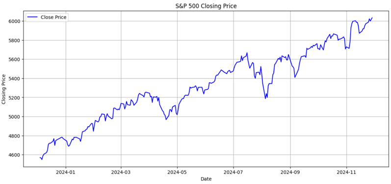
From Figure 2, overall, the index can be seen to follow a broadly upward trajectory despite several short-lived corrections, finishing the period substantially higher than it began. The most notable movements include a mid-year surge and a sharp dip in late August, both of which temporarily interrupted the general rise.

At the start of the period, the S&P 500 traded at roughly 4,550 points. It climbed steadily over the first quarter, reaching around 5,200 by late March. Although prices briefly faltered in April, the index regained momentum and accelerated through early summer, peaking at approximately 5,650 in July. This was followed by the steepest decline on the chart: a sudden fall to just above 5,200 in late August, representing a drop of more than 400 points.

However, the market recovered quickly. From September onward, the index resumed its ascent, surpassing 5,800 in October and breaking the 6,000-point threshold in November. It ended the year at a record high of slightly above 6,050.

In summary, despite intermittent volatility, the S&P 500 experienced robust and sustained growth across 2024, closing the year at a level around 1,500 points higher than its value in December 2023.

Figure 2 | The change in the S&P 500 index

Models Evaluation and Comparison

This section provides comparison between our forecasting model’s prediction and that of the ARIMA(p,d,q), Double Exponential Smoothing, and ANN models in making prediction for stock closing price at t + 1, t+3 and t+5 (one day, three days, and five days after the last date in the training sets, respectively) of the S&P 500 individual stocks. We evaluated the models’ performance using the mean absolute error (MAE) and the mean absolute percentage error (MAPE).
Definition 4.1 The mean absolute error for predictions for $t+N$ ( $MAE_N$ ) is calculated as

(23) $\begin{equation*}MAE_N = \frac{\sum_{t=1}^n |P_{true}(t+N) - P_{predicted}(t+N)|}{n}\end{equation*}$

where $n$ is the number of predictions, $P_{true}(t+N)$ is the true price at time $t+N$ , and $P_{predicted}(t)$ is the predicted price at time $t+N$ .

Definition 4.2 The mean absolute error for predictions for $t+N$ ( $MAPE_N$ ) is calculated as

(24) $\begin{equation*}MAPE_N = 100\% * \frac{1}{n} \sum_{t=1}^n \left| \frac{P_{true}(t+N) - P_{predicted}(t+N)}{P_{true}(t+N)} \right|\end{equation*}$

where $n$ is the number of predictions, $P_{true}(t+N)$ is the true price at time $t+N$ , and $P_{predicted}(t)$ is the predicted price at time $t+N$ .

Since the Kinetic Energy-based model is stochastic, its predictions are slightly different each time it is run. To compare with other models, which are deterministic, we estimate the population MAEs, and MAPEs for the Kinetic Energy-based model using the 95% confidence interval from 30 runs. Since the MAEs and MAPEs are averaged from the errors of the prediction for 500 stocks, by the Central Limit Theorem²³ this sample size (500) is large enough for the distribution of the MAEs and MAPEs from 30 runs to be approximately normal, regardless of their individual underlying errors’ distribution. Therefore, the computation for the 95% confidence intervals applies.

Definition 4.3 The 95% confidence intervals for a variable X is calculated respectively as CI_{X 95%}such that

(25) $\begin{equation*}CI_{X 95\%} = \widehat{\mu_X} \pm t^* SE_{\widehat{X}}\end{equation*}$

Where $\mu_X$ is the mean of some $n$ number of $X$ , $t^*$ is the t-multiplier for 95% confidence, and $SE_{\widehat{X}}$ is the standard error of the $n$ number of $X$ .

Table 7 shows the performance comparison of forecasting models for S&P 500 stocks’ closing price at time one day, three days, and five days after the last date of the training sets, namely the $MAE_1$ , $MAE_3$ , $MAE_5$ , $MAPE_1$ , $MAPE_3$ , and $MAPE_5$ . Note that the metrics (MAE and MAPE) for the Kinetic Energy-based model is the 95% confidence interval of its metrics from 30 runs, namely the $CI_{MAE 95\%}$ and $CI_{MAPE 95\%}$ from Definition 4.3.

	Performance for t+1 prediction		Performance for t+3 prediction		Performance for t+5 prediction
Model	MAE	MAPE	MAE	MAPE	MAE	MAPE
KE-based	(2.187, 2.222)	(0.92%, 0.93%)	(10.654, 11.467)	(4.240%, 4.410%)	(13.034, 13.881)	(5.430%, 5.590%)
ARIMA(p,d,q)	2.451	1.168%	3.00	1.460%	3.728	1.816%
Double Exponential Smoothing	2.598	1.240%	3.059	1.550%	4.1355	2.00%
ANN	7.016	3.170%	10.795	4.540%	11.958	5.220%

Table 7 | Performance comparison of forecasting models for S&P 500 stocks’ closing price at time t+1, t+3, and t+5

According to the results shown in Table 6, for the prediction for 1-day ahead, the Kinetic Energy-based model resulted in a better performance than all of the other three models, with the 95% confidence interval for MAEs and MAPEs less than the MAEs and MAPEs from the other three models. In other words, it is with 95% confidence that the population MAE and MAPE resulting from the Kinetic Energy-based model are less than the MAEs and MAPEs from the other three models. However, for the prediction for 3-day ahead, the ARIMA(p,d,q) and Double Exponential Smoothing model did better than the Kinetic Energy-based model, while the ANN model did about the same as the Kinetic Energy-based model in terms of MAE and MAPE. For the prediction for 5-day ahead, the ARIMA(p,d,q) and Double Exponential Smoothing model also did better than the Kinetic Energy-based model, while the ANN model did slightly better than the Kinetic Energy-based model in terms of MAE and MAPE.

Besides comparing the model’s performance in predicting the future closing prices, we also compared the model’s performance in trading the S&P 500 stocks. The first comparison we looked at is the model’s returns when compared against the S&P 500 index itself. Note that for back testing purposes and the limitation of data, we assume single-agent market, meaning we are the only one who traded stocks on daily resolution, using daily closing price as execution price for all trades. The formula for the return for N-day holding is expressed in Definition 4.4 with a naive trading algorithm using signals of -1 and 1. To be specific, if the model predicts a positive change in the closing price after N days, then it will buy and hold for N days (go long), else if the model predicts a negative change in the closing price after N days, then it will sell the stocks (go short).

Definition 4.4 Given a signal generated by a model, where signal =-1 (indicating sell) if prediction for P_t+N < P_t, and signal =1 (indicating buy) if prediction for P_t+N > P_t, the return for N-day holding is calculated as follows

(26) $\begin{equation*}R_{t+N} = signal_t \frac{P_{true}(t+N) - P_{true}(t)}{P_{true}(t)}\end{equation*}$

Using the models, we then compared the mean return for N-days holding using prediction of t+N for all S&P 500 stocks with the mean return of the S&P 500 index after N-day. Table 7 shows the comparison for the mean S&P 500 stocks return for 1-day, 3-days, and 5-days holding of the models using t+1, t+3, and t+5 predictions, respectively, and the S&P 500 index. Note that for the Kinetic Energy-based model, the results are in the 95% confidence interval from 30 runs, following the similar computation method from Definition 4.3 (the mean returns are from a sample of 500 stocks so Central Limit Theorem applies, meaning the distribution of the mean returns are approximately normal, thus the computation for the 95% confidence interval applies). Note that the models and the S&P 500 index were evaluated on the entire test set.

Model	1-day holding	3-days holding	5-day holding
KE-based	(0.0950%, 0.103%)	(0.0013%, 0.0617%)	(0.159%, 0.262%)
ARIMA(p,d,q)	-0.375%	-0.0831%	-0.140%
Double Exponential Smoothing	-0.355%	0.0314%	0.0619%
ANN	-0.163%	-0.397%	-0.670%
S&P 500 index	0.112%	0.113%	0.111%

Table 8 | Comparison of the models’ mean return for S&P 500 stocks and S&P 500 index for t+1, t+3, and t+5

According to the results shown in Table 7, the Kinetic Energy-based model overall has higher mean returns than the other traditional models when evaluated for 1-day, 3-days, and 5-days holding ahead using t+1, t+3, and t+5 predictions, respectively (except when compared to Double Exponential Smoothing model for 3-days holding). For 1-day and 3-days holding using t+1 and t+3, respectively, the Kinetic Energy-based model’s mean return is less than that of the S&P 500 index, while for 5-days holding, the Kinetic Energy-based model’s mean returns are greater than that of the S&P 500 index.

The second metric for trading we employed to compare the models is the Sharpe Ratio²⁴ , which is a financial metric that measures the risk-adjusted return of an investment: the higher the value, the better the risk-adjusted return. The formula for the Sharpe Ratio is expressed in Definition 4.5.

Definition 4.5 Given the average return of a portfolio R_p, the risk-free return R_f, and the standard deviation of the portfolio excess return (volatility) σ_p, the Sharpe Ratio is calculated as follows

(27) $\begin{equation*}Sharpe Ratio = \frac{R_p - R_f}{\sigma_p}\end{equation*}$

We compared the models’ Sharpe Ratios using the t+1 prediction (daily) and traded for 7 days, 10 days, and 30 days. The reason we used the t+1 prediction for the trading signal was because from Table 7, among all time horizons (t+1, t+3, and t+5), the t+1 prediction for the Kinetic Energy-based model produced the best mean returns. Therefore, we wanted to compare the models in the scenario when the Kinetic Energy-based model did at its best. Note that this back testing procedure also assumes single-agent market using daily closing price as execution of price for all trades. To find the value for the risk-free return $R_f$ , we derived it from the value of 4.37% or 0.0437 for the annual risk-free return reported recently as of February 6, 2025 by the U.S. Department of The Treasury²⁵ _. Assuming there are 252 trading days in a year²⁶ , the daily risk-free return is about 0.0173. Table 8 shows the comparison for the models’ Sharpe Ratios when traded for 7 days, 10 days, and 30 days on all S&P 500 stocks using the t+1 prediction for generating buy and sell signals. Note that the for the Kinetic Energy-based model, the results are in the 95% confidence interval from 30 runs, following the similar computation method from Definition 4.3 (the portfolio or global Sharpe Ratio was calculated from the mean returns of 500 stocks so the Central Limit Theorem applies, meaning the distribution of the mean returns are approximately normal, thus the computation for the 95% confidence interval applies). Note that the models were evaluated on 7-days, 10-days, and 30-days into the test set.

Model	7-days Sharpe Ratio	10-days Sharpe Ratio	30-days Sharpe Ratio
KE-based	(0.159, 0.166)	(0.0425, 0.0492)	(0.0120, 0.0141)
ARIMA(p,d,q)	-0.787	0.0494	-0.0537
Double Exponential Smoothing	1.444	1.170	1.220
ANN	0.2758	0.1591	0.132

Table 9 | Comparison of the models’ Sharpe Ratios when traded for 7 days, 10 days, and 30 days on all S&P 500 stocks using the t+1 prediction for generating buy and sell signals.

According to the results shown in Table 8, the t+1 predictions made by ANN model overall resulted in the highest Sharpe Ratios when used to trade for 7 days, 10 days, and 30 days. The t+1 predictions made by the Double Exponential Smoothing model overall resulted in the second highest Sharpe Ratios when used to trade for 7 days, 10 days, and 30 days. When used to trade for 7 days and 30 days, the predictions of the Kinetic Energy-based model resulted in greater Sharpe Ratios than those of the ARIMA(p,d,q) model.

Discussion

In this section, we discuss the strengths and weaknesses of our stock closing price forecasting model.

Strengths

The first strength that our model has is its consideration of the amount of trading volume. As mentioned, the trading volume has an effect on the behavior of the stock price. The greater the trading volume, the greater the kinetic energy, which likely increases the stock price after some time. By using kinetic energy, our model is able to incorporate such a relationship between the trading volume and stock price to predict the future prices. This exploitation of the kinetic energy explains the better accuracy in our model’s predictions compared to that of some of the other models when predicting the closing prices for 1 day ahead.

The second advantage that our model has is its simplicity. Our model relies on the idea of kinetic energy which can be computed easily. The only variables needed to be estimated are the future kinetic energy, the trading volume, and the weight β for the weighted average between the Monte Carlo simulation and the mean of the recent closing prices. Our model also allows for tuning the number of simulations. Given such simplicity and flexibility, traders can implement this model with ease and with the ability to tune it.

Weaknesses

The first weakness that we observe in our model is its method to calculate the future kinetic energy and the trading volume. Since such calculations rely on random variables from the distribution of kinetic energy and trading volume themselves, the prediction is not deterministic but rather stochastic, generating different results each time the simulations are run. The number of simulations also influences the performance of the model. In particular, increasing the number of simulations improves the model’s performance by generating a more stable estimation of future kinetic energy and trading volume. However, as the number of simulations increases, the time taken to run them will also increase, which can hinder the trading process in situations where high frequency trading is required. Therefore, traders should take this trade-off into consideration when tuning the model.

The second weakness that our Kinetic Energy-based model has is its unreliability in predicting the closing prices on the long time horizon. From the results in Section 4.2, it can be seen that the model outperforms other traditional models when forecasting closing prices for 1-day ahead. However, it did worse than other models when forecasting closing prices for 3-days and 5-days ahead. These results indicate that the Kinetic Energy-based model is more applicable in predicting short-term changes rather than long-term changes in closing price. For long trading periods, the Kinetic Energy-based model underperforms the Double Exponential Smoothing and ANN model in terms of Sharpe Ratios, even though the Kinetic Energy-based model outperforms the Double Exponential Smoothing and ANN model in terms of mean returns for holding N-days. The reason is due to the fact that the Kinetic Energy-based model predicts possible values of variables (e_KE and e_m) from their past distributions and is stochastic, which results in higher volatility. These results show that generally, while the Kinetic Energy-based model is better than some other models at generating returns on trades, its returns are not as stable as those of some other models. Therefore, using the Kinetic Energy-based model, traders should take these characteristics into consideration to decide whether they want to trade for a short-term period or invest for a long-term period, and whether they want to maximize the return or minimize the risk.

Conclusion

In this research paper, we investigated the changing of the S&P 500 index from December 6, 2023, to December 2, 2024. We then developed a model to predict the future value of the stock closing price for the S&P 500 companies based on the idea of kinetic energy. Our model is evaluated with the ARIMA(p,d,q), Double Exponential Smoothing, and ANN model using the mean absolute error (MAE) and the mean absolute percentage error (MAPE). The models were then evaluated on the mean returns for 1-day, 3-days, and 5-days holding, using t+1, t+2, and t+3 predictions, respectively. Using the t+1 predictions, the models were also evaluated using the Sharpe Ratios for 7 days, 10 days, and 30 days of trading.

Overall, the S&P 500 index showed an upward trend with slight fluctuation throughout the period. In forecasting future stock closing prices for one day ahead, the Kinetic Energy-based model resulted in higher accuracy than the other forecasting models. To be specific, in predicting the price the day after the last date of the training set of the S&P 500 stocks, the Kinetic Energy-based model got MAEs and MAPEs in their 95% confidence intervals of (2.187, 2.222) and (0.92%, 0.93%). In general, the Kinetic Energy-based model was better at generating returns, while it underperformed some other models in the stability of those returns. Therefore, from these results, the Kinetic Energy-based model is generally better for short-term forecasting, and for maximizing the returns on trades, but it is not as good for long-term forecasting, and minimizing the risks that those returns have. It is also worth noting that the algorithm used for evaluating the model’s performance in terms of mean returns and Sharpe Ratio was naive for generating signals. In other words, the signals for buy and sell depended purely on whether the models predict a positive or negative change for the future prices. Therefore, it is recommended that traders and researchers experiment with and optimize some thresholds that can trigger the signals for buy and sell more efficiently.

Appendix

Below is the pseudocode for the KE-based model in predicting future prices at time t+N.

References

A., Rjumohan. Stock Markets: An Overview and A Literature Review. Munich Personal RePEc Archive (April 2019). https://mpra.ub.uni-muenchen.de/ 101855/1/MPRA_paper_101855.pdf [↩]
Mehar Vijh a, Deeksha Chandola, Vinay Anand Tikkiwal, and Arun Kumar. Stock Closing Price Prediction using Machine Learning Techniques. Procedia Computer Science (2020). https://www.sciencedirect.com/science/article/pii/ S1877050920307924?ref=pdf_download&fr=RR-2&rr=925f6ab34f39b039 [↩] [↩] [↩] [↩] [↩] [↩]
Bhargava R. Kotur. Kinetic Energy of a Particle Independent of its Mass & Velocity. IOSR Journal Of Applied Physics (2023). https://hal.science/ hal-03975986/document. [↩] [↩]
Kiyoshi Kanazawa, Takumi Sueshige, Hideki Takayasu, and Misako Takayasu. Kinetic Theory for Finance Brownian Motion from Microscopic Dynamics (February 2018). https://arxiv.org/pdf/1802.05993 [↩] [↩] [↩]
Mahdieh Ghotbi and Morteza Zahed. Predicting Price Trends Combining Kinetic Energy and Deep Reinforcement Learning. SSRN (July 2023). https://papers. ssrn.com/sol3/papers.cfm?abstract_id=4502473. [↩] [↩] [↩]
Sidharth Tiwary and Pramod K. Mishra. Time-series Forecasting of Stock Prices using ARIMA: A Case Study of TESLA and NIO. Industrial Engineering and Operations Management Society (August 2022). https://ieomsociety.org/ proceedings/2022india/427.pdf. [↩] [↩] [↩]
Md Aminur Rahman. Forecasting Stock Prices Through Exponential Smoothing Techniques in The Creative Industry of The UK Stock Market. International Journal of Asian Business and Management (2024). https://journal. formosapublisher.org/index.php/ijabm/article/view/9104/9778. [↩] [↩] [↩]
yfinance library. https://pypi.org/project/yfinance/. [↩]
Andreea-Cristina Petrica, Stelian Stancu, and Alexandru Tindeche. Limitation of ARIMA models in financial and monetary economics. Theoretical and Applied Economics (2016). https://www.ebsco.ectap.ro/Theoretical_&_ Applied_Economics_2016_Winter.pdf#page=19. [↩]
Humberto Lopez. The power of the ADF test. Economics Letters (November 1997). https://www.sciencedirect.com/science/article/abs/pii/ S0165176597818721. [↩]
Shane Allua, PhD, and Cheryl Bagley Thompson, PhD, RN. Hypothesis Testing. Air Medical Journal. https://www.airmedicaljournal.com/article/ S1067-991X(09)00068-6/pdf. [↩]
Results for the ADF test on original training sets of the S&P 500 stocks. https://docs.google.com/spreadsheets/d/1MaTkz3svU_ gw9HZHmhKBURaSxaCysXYLixNJW-uLAfk/edit?usp=sharing [↩]
Results for the ADF test on first order differenced training sets of the S&P 500 stocks. https://docs.google.com/spreadsheets/d/ 1GpkcesJtYzod4kkEqveWRBt87AX0Tib9B1Jbur_NVhc/edit?usp=sharing. [↩]
G. M´elard and J.-M. Pasteels. Automatic ARIMA Modeling Including Interventions, Using Time Series Expert TSE-AX software. ResearchGate (October 2000). https://www.researchgate.net/publication/223078338_Automatic_ARIMA_modeling_including_interventions_using_time_series_expert_software. [↩]
Results for the optimal parameters for the ARIMA(p,d,q) of the training sets of the S&P 500 stocks. https://docs.google.com/spreadsheets/d/ 1l6s5M6rUbcAtnq-OPY0mLdpMFK9jwXXNxgteOIyx-Zc/edit?usp=sharing. [↩]
Results for the optimal parameters for the Double Exponential Smoothing of the training sets of the S&P 500 stocks. https://docs.google.com/spreadsheets/d/1IlcRXMSiRuC0IzvxnsgzOnODeF9qTpjF4X-6Cl37t8k/edit?usp=sharing. [↩]
Keras, RandomSearch Tuner, https://keras.io/keras_tuner/api/tuners/random/ [↩]
Diederik P. Kingma and Jimmy Lei Ba. ADAM: A METHOD FOR STOCHASTIC OPTIMIZATION. International Conference on Learning Representations (2015). https://arxiv.org/pdf/1412.6980. [↩]
Jackson Dino. The Effect of Trading Volume on Stock Price. Gettysburg College Headquarters (2023). https://cupola.gettysburg.edu/cgi/viewcontent.cgi? article=1032&context=gchq. [↩]
S. S. Shapiro and M. B. Wilk. An Analysis of Variance Test for Normality (Complete Samples). Biometrika (1965). https://www.math.utah.edu/~morris/Courses/ShapiroWilk.pdf [↩]
Samik Raychaudhuri. INTRODUCTION TO MONTE CARLO SIMULA- TION. Winter Simulation Conference (2008). https://www.informs-sim.org/wsc08papers/012.pdf. [↩]
GPU machine types. https://docs.cloud.google.com/compute/docs/gpus?utm_source=chatgpt.com [↩]
Sang Gyu Kwak and Jong Hae Kim. Central limit theorem: the cornerstone of modern statistics. National Institutes of Health (2017). https://pmc.ncbi.nlm.nih.gov/articles/PMC5370305/ [↩]
William F. Sharpe. The Sharpe Ratio. The Journal of Portfolio Management (1994). https://web.stanford.edu/~wfsharpe/art/sr/sr.htm [↩]
Daily Treasury Rates. U.S. Department of The Treasury (2025). https://home.treasury.gov/resource-center/data-chart-center/interest-rates/TextView?type=daily_treasury_yield_curve&field_tdr_date_value=2025 [↩]
Number of Trading Days per Year. macroption. https://www.macroption.com/trading-days-per-year/ [↩]

Stock Closing Price Prediction Using Kinetic Energy and Stochastic Processes

Abstract