Exploring The Weightage of Correlates of Diabetes Using Machine Learning

Aarush Raheja¹, Adam Li^2
1 Student Researcher, Symbiosis International School, Pune, India
² Research Mentor, PhD at Johns Hopkins University

Abstract

There is an increase in the prevalence of Type 1 and Type 2 Diabetes around the world. This alarming trend highlights the need for prediction tools that can help identify risk factors associated with these chronic diseases, so that interventions can be implemented at a much earlier stage in their development. This study investigates two distinct datasets drawn from Kaggle, focusing on clinical and lifestyle factors, respectively. We constructed machine learning models, such as Logistic Regression L1 penalty, Logistic Regression L2 penalty, Random forest and a dummy classifier model to contrast basic accuracy, to first make predictions of the likelihood of diabetes occurrence given various factors. We demonstrate that the models have high predictive accuracy, with the logistic regression L2 penalty model achieving 95.297% accuracy, the logistic regression L1 penalty model achieving 96% accuracy, and the random forest model achieving 97% accuracy. However, the key contribution of this study is to provide interpretation of these models to determine the most important drivers of the models’ predictions. We find that even though well-known factors such as HBA1C level, hypertension, and heart disease have high associations with diabetes, factors such as mental health even though below BMI and HBA1C level do have a moderate predictive power.

Introduction

Diabetes is a disease that affects 500 million people worldwide and constitutes a major public health crisis. To predict individual propensity toward developing diabetes, traditional methods include HBA1c testing and fasting glucose levels. However, these methods are time consuming, invasive, resource intensive and often impractical for large scale screening¹. Identifying the key factors contributing to diabetes risk at the population level is important, as this will enable policy makers and public health experts to determine the most effective interventions.

To address this challenge, machine learning methods can be used to identify specific factors that determine the incidence of diabetes. Many ML models have shown promising results in the prediction of diabetes, such as studies by Lugner², health administration data models³, and detailed lifestyle-only modeling⁴. However, these studies only focus on a minimal number of variables and often fail to include lifestyle factors – such as smoking, physical inactivity, alcohol use, and dietary patterns – that have a known relationship to diabetes risk. In addition, these studies commonly focus on optimizing a performance metric but provide little information about the most important factors driving the model’s performance⁵. For example, the study by Noh⁶ explores factors such as BMI, HBA1C but does not explore basic lifestyle factors such as the physical activity of the individual. The study by Mohsen et al.⁷, while incorporating similar factors does not provide insight into which factors are most determinative of the model’s predictive power. Additionally, there are several examples such as Zhou⁸, Negi⁹ and Alhussan¹⁰ that encompass less than 10 features while predicting diabetes thus not being able to access the full range of factors that affect it.

Recent studies have further expanded the application of machine learning to diabetes prediction. Tasin et al. developed a prediction system incorporating explainable AI techniques, finding that ensemble methods outperformed individual classifiers on the Pima Indian dataset¹¹. Rajendra and Latifi demonstrated that logistic regression combined with ensemble approaches could achieve competitive accuracy for diabetes classification¹². Edlitz and Segal developed logistic regression-based scorecards for predicting type 2 diabetes onset, highlighting the interpretability advantage of simpler models¹³. Wang compared random forest and logistic regression models specifically for diabetes prediction, finding that tree-based models significantly outperformed linear models on clinical data¹⁴. Abousaber evaluated multiple classifiers on imbalanced diabetes datasets and found that resampling techniques such as SMOTE significantly improved recall for the minority class¹⁵. Additionally, Ganie and Malik demonstrated that ensemble approaches incorporating oversampling could boost classification performance for lifestyle-based diabetes indicators¹⁶. These findings underscore the importance of addressing data imbalance and using multiple evaluation metrics when interpreting model performance.

To address these limitations, this study analyzes a broad range of lifestyle factors and also provides interpretation of each of the models used to determine the most important variables. Here, we test a wide variety of common machine learning frameworks, including logistic regression (with both L1 and L2 regularization) and random forests on two distinct datasets. The first one focuses on clinical factors, whereas the second one includes primarily lifestyle factors to expand the range of factors of the study. Rather than aiming for optimization, this study utilizes the factors to answer a more nuanced question of which range of factors are better predictive of whether the patient has diabetes or not, which gives insight into which factors are most influential with respect to diabetes prediction.

The results show that the random forest model achieved the highest accuracy – 97% on the first dataset. While the logistic regression with L1 regularization did not perform as well it still offers interpretable insights into the key contributing factors in both datasets. In addition to well known factors such as HbA1c level and BMI, factors such as smoking, alcohol consumption and mental health also emerged as important drivers. These findings open a pathway to diabetes prediction in the future, ensuring that diabetes prediction in the future is based on a vast range of factors that can be accounted for and changed easily.

Motivation

The global prevalence of diabetes has risen sharply over recent decades. Even though as individuals we are aware of the factors that affect us and cause diabetes the global rate still has yet to take a hit. With blood glucose levels and BMI being at the top of our list there are several other factors that aren’t considered. Thus this study aims to delve deeper into these factors and identify how vital they are when it comes to predicting whether a patient has diabetes or not through numerous machine learning models. Alongside this as a personal motivation, both my parents are diabetic as well putting me as an individual also at high risk, knowing this research allows me to understand what other factors there are that can push me towards developing this disease whether it be smoking, alcohol consumption, mental health, etc.

Methods

Datasets

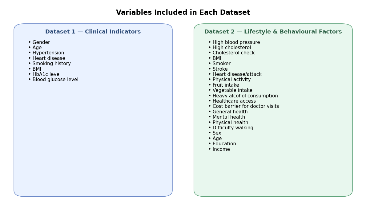
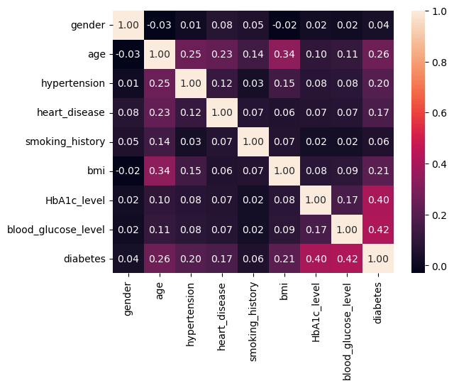
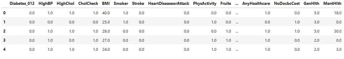
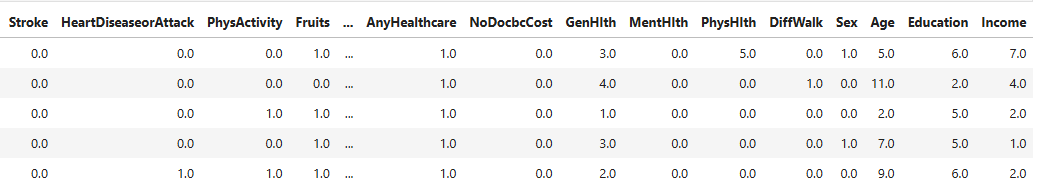
Datasets for this study were obtained from publicly available sources. The first dataset contains factors such as: gender, age, hypertension, heart_disease, smoking_history, bmi, HbA1c_level and blood_glucose_level to predict a final outcome of whether the patient has diabetes or not. The second dataset contains other factors such as: HighBP (Blood Pressure), HighChol (Cholesterol), CholCheck (Cholesterol Check), BMI (Body mass Index), Smoker, Stroke, HeartDiseaseorAttack, PhysActivity (Physical Activity), Fruits, Veggies, HvyAlcoholConsump (Heavy Alcohol Consumption), AnyHealthcare, NoDocbcCost (Was there a time in the past 12 months when you needed to see a doctor but could not because of cost? 0 = no, 1 = yes), GenHlth (General Health), MentHlth (Mental Health), PhysHlth (Physical Health), DiffWalk (Difficulty to walk), Sex, Age, Education, Income.

Notably many of dataset 2’s variables were binary (eg: smoker vs non-smoker, Heavy alcohol consumption vs not heavy alcohol consumption). These coarse categories could reduce the predictive abilities of models to capture variation within behaviour, thus limiting the predictive performance of this dataset.

Data Preprocessing and Missing Value Analysis

Data Preprocessing is an integral part of any machine learning model. During the course of this research after reviewing the entire data set thoroughly little data was removed; data values that were missing were marked with “no info”. Missing data handling remains a critical yet often underreported step in machine learning prediction studies^17,18. Nijman et al. found that a majority of machine learning prediction studies do not adequately report their missing data strategies¹⁷, underscoring the importance of transparent reporting.

No features and no samples were removed as the number of instances of this occurring were minimal and had a negligible effect on the machine learning model. However, encoding these values as “no info” in a few places may have introduced bias by treating absence of data as a valid category which could introduce noise since the model could interpret the absence of data as predictive information. While this, in turn, did enable the preservation of most of the dataset for training, more rigorous imputation techniques (eg: mean/mode imputation or k nearest neighbors) could be explored in the future to assess whether they improve performance and reduce noise.

Dataset	Total Samples	Missing Values	Handling
Dataset 1 (Clinical)	100,000	Minimal (“No Info” in smoking_history)	Encoded as “No Info” category
Dataset 2 (Lifestyle)	253,680	None (pre-cleaned BRFSS data)	No imputation required

Encoding and Train-Test Split

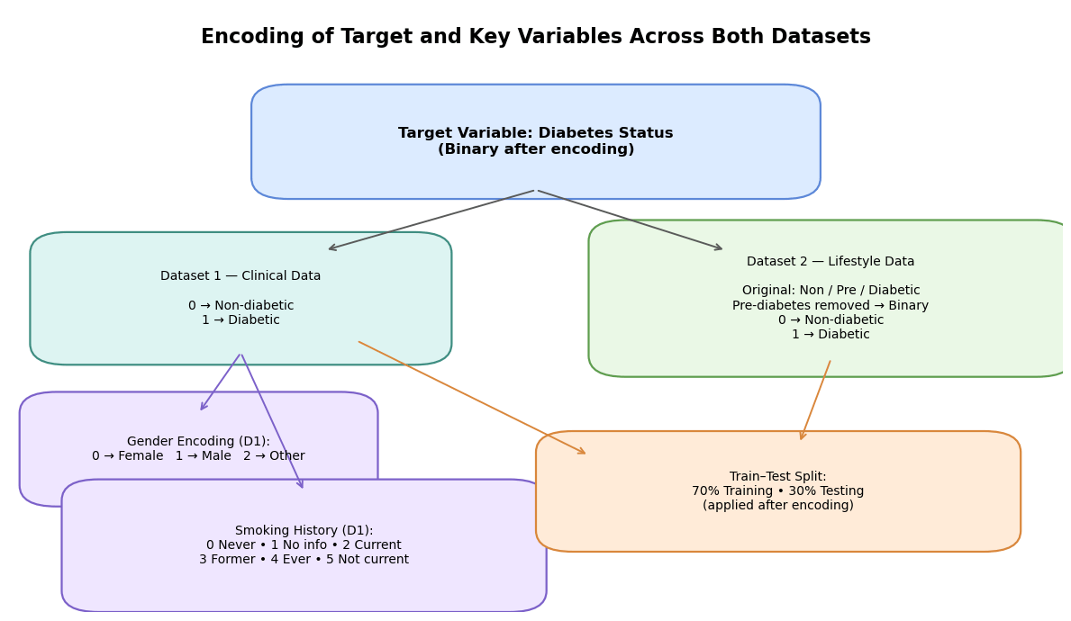
Categorical variables were encoded numerically to allow machine learning model process data. Variables that held a string value were encoded into different integer categories, a process which is described in the latter part of this paper. The Target variable for this research was whether the patient had diabetes – for the first dataset healthy patients were encoded with “0” while as diabetic patients were encoded with a “1”. Other variables that were encoded were gender where “0” represented female, “1” represented male and “2” represented another category. Furthermore, smoking history was also encoded where “0” represented never, “1” represented no info, “2” represented current, “3” represented former, “4” represented ever and “5” represented not current. For the second dataset however there was a change. Even though the target variable was the same, diabetes, there was an additional category for pre-diabetes which was removed to allow the target variable to be classified into a binary outcome, allowing comparison with data set 1 which only had this binary target variable. “0” was encoded as non-diabetic and “1” was encoded as diabetic. For this particular model the split between training and testing data was 70:30.

Cross-Validation and Evaluation Metrics

Alongside this a simple cross-validation was used to evaluate model performance. Each model was trained on 4 folds and tested on the remaining fold, rotating across all folds. This approach provided an estimate of mean accuracy across all folds. However, stratification by class labels was not applied meaning that folds may have contained imbalanced distributions of diabetic vs non-diabetic cases.

Also, other evaluation metrics such as precision, recall, F1 score and ROC-AUC were used to provide a whole assessment of the models’ performance. Precision quantified how many patients predicted as diabetic were actually diabetic, while recall measured the proportion of true diabetic cases correctly identified. F1 score balanced these two metrics into a single measure of performance while the ROC-AUC allowed to understand the models’ discrimination ability across thresholds¹⁹.

To assess the variability and assess the robustness of the model performance, we computed 95% confidence intervals for all evaluation metrics using bootstrap resampling. For each model we sampled with replacement from the test set over 1000 iterations and recalculated accuracy, precision, recall, F1 score and ROC-AUC. This procedure provided estimates of the stability of each metric, ensuring that reported performance was not due to random variation in a single train-test split.

Dataset 1 in this instance exhibited class imbalance, with a larger proportion of non-diabetic cases to diabetic cases. No balancing techniques such as SMOTE oversampling, undersampling or class weights were applied in this study. Instead, the models were evaluated using cross validation to mitigate overfitting, but future work should directly test balancing strategies to assess their impact on predictive stability.

Model Descriptions

To predict an outcome this study uses models like Decision tree, Random forest, Logistic regression and logistic regression with an L1 penalty to train and develop the model to a higher accuracy.

Logistic Regression

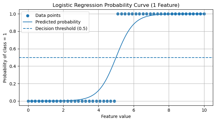
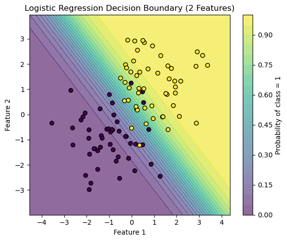
Logistic Regression model is a well-known and widespread model that makes a binary classification. It is somewhat similar to the linear model although the logistic regression model generates a probability value ranging between 0 and 1 on how likely the data point is to fit into the classification of a success or a failure. This probability is then compared to a threshold value, and based on the probability deciphered a final output is given whether the model predicts true or false.

Logistic Regression (L1 Penalty)

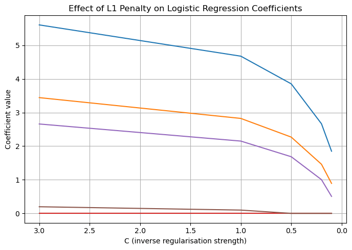
Logistic regression using an L1 penalty applies a penalty proportional to the absolute value of the coefficients. This, in turn, drives non predictive factors to zero, resulting in a sparse model. Such sparsity enables effective feature selection, allowing only the highest weighted correlates to affect the model’s accuracy.

As described in the CS Extended Essay, logistic regression with L1 penalty estimates the probability that a person has diabetes based on their features, producing a probability between 0 and 1. However, when many variables are included, some may add noise rather than useful information. The L1 penalty fixes this by gradually forcing weaker variable coefficients to zero. This behaviour is valuable for this investigation because it highlights which factors consistently remain important when the model is encouraged to be selective. In the context of diabetes, this helps identify the strongest contributors rather than maximizing accuracy^12,13.

Logistic Regression (L2 Penalty)

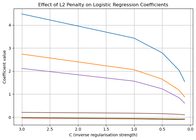
Logistic regression using the L2 penalty applies a squared penalty to the coefficients although not to zero. Unlike L1 it does not perform feature selection but instead stabilises the model, while retaining all predictive features.

In contrast to L1, L2 regularization doesn’t push coefficients all the way to zero. Instead, it gently shrinks all coefficients smaller in magnitude. This means that instead of driving any coefficients exactly to zero, L2 spreads the regularization evenly across all coefficients. Because of this, L2 regularization tends to create models where all the features are included, but none of them have extremely large coefficients. This makes L2 particularly useful when we want to keep all the features in the model, but still control how much influence each one has. This makes L2 especially useful where we want to control the overall influence of all features rather than eliminating any of them – a feature that is particularly useful while investigating lifestyle factors.

Random Forest

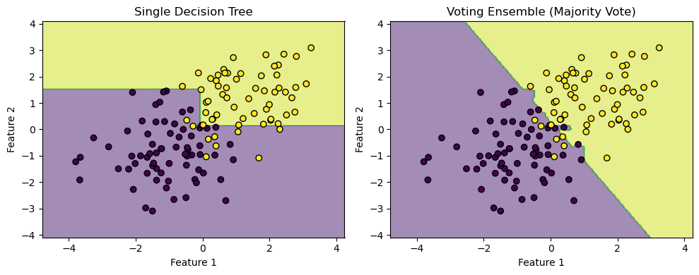
A random forest model is a combination of decision tree models that work on the concept of a series of questions that classify an input into categories. Each decision tree has several nodes, nodes that represent question making classifying the input further. Although this model is sometimes prone to overfitting which can hamper the results. The model employed consisted of 100 trees; Gini impurity as the splitting criterion, and no maximum depth restriction, meaning trees were allowed to grow until the leaves were pure. The choice of 100 trees was a reflection of prior successful application of random forest models in medical datasets. Additionally, allowing unrestricted depth minimized bias, though at risk of overfitting which was mitigated by cross-validation.

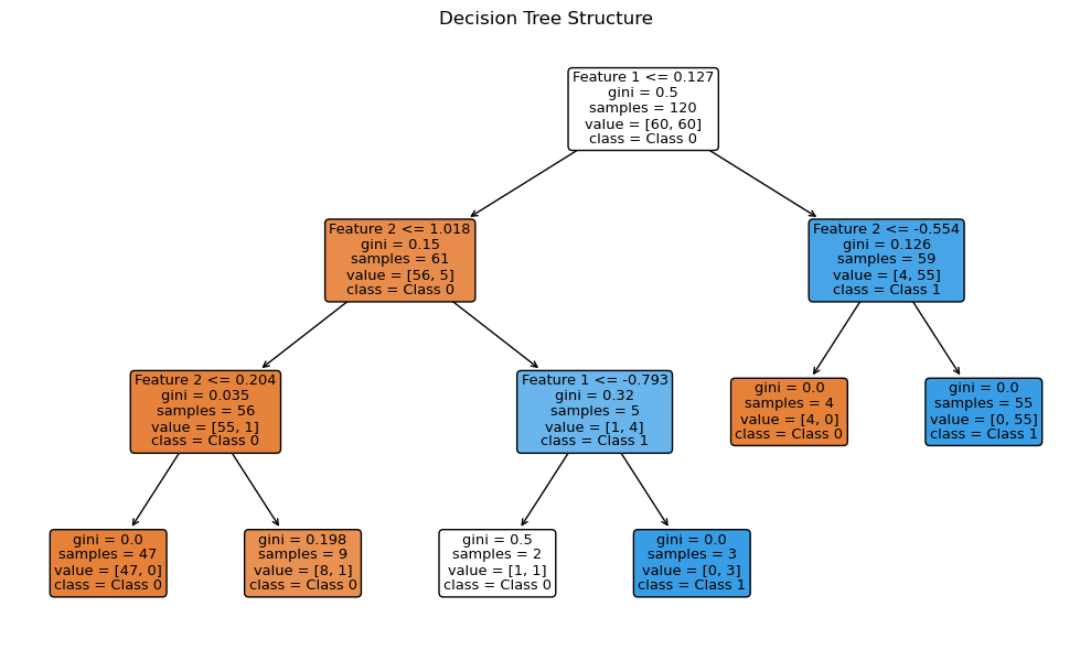
Decision trees are the building blocks of a random forest. Each decision tree learns by splitting the data into smaller groups. It does this step by step using simple questions about the features. At each point, the tree picks a feature and a threshold that best splits the data into classes. Eventually, the tree forms a series of branches that lead to final decisions at the leaves.

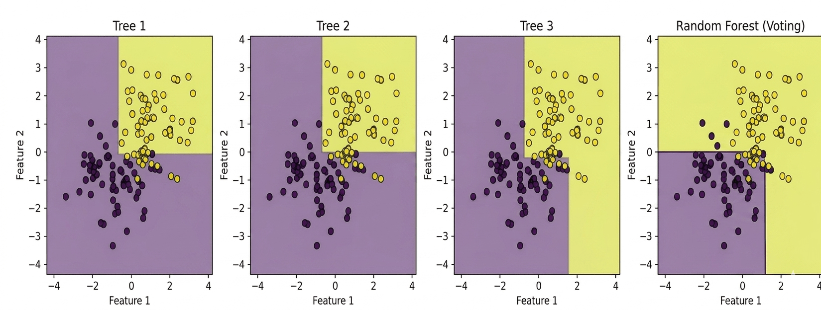
Ensemble learning is a technique where multiple models are combined to produce a stronger overall prediction. By aggregating the predictions of several models, ensemble learning can achieve better performance than any individual model alone. In the case of a random forest, multiple decision trees are trained on different subsets of data. Each of these trees votes on the final prediction, and the majority vote determines the final decision. This approach reduces the risk of overfitting and often leads to a more robust and accurate model.

Dummy Classifier

The dummy classifier included as a baseline, highlighted dataset imbalance by achieving high accuracy (91.67%) while failing across recall and precision. The dummy classifier is a baseline model that makes predictions using simple rules, such as always predicting the most frequent cases. It doesn’t learn from the data and often serves as a performance benchmark for more complex models.

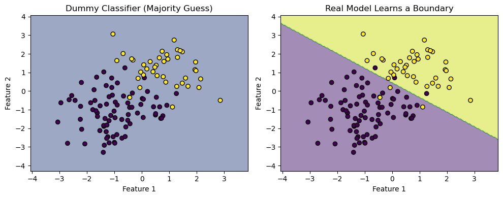
In current clinical practice, diabetes risk is frequently assessed using established scoring systems such as the ADA risk test, FINDRISC or Qdiabetes. These models rely on simple additive rules based on demographic and lifestyle factors, which makes them interpretable but also limited in their ability to capture complex non-linear relationships. Our study did not directly compare ML models to these clinical scores, instead we employed a dummy classifier as a baseline to establish the minimum threshold of predictive value. This approach allowed us to quantify the relative improvement achieved by different ML methods. However future work should benchmark machine learning models against clinical scoring systems to provide a more direct assessment of their added value in practice^20,19.

Procedure

The experimental procedure followed these steps:

Data Set 1

Results – Dataset 1

These results should be interpreted cautiously however, as the class imbalance of the first dataset may have contributed to inflating the accuracy of these models. The dummy classifier achieving 91.667% highlights this imbalance.

MODEL	Accuracy	Precision	Recall	F1-score	ROC-AUC
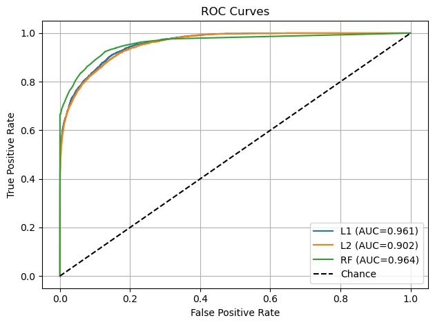
LR L1	96%	0.88	0.60	0.72	0.961
LR L2	95.297%	0.74	0.48	0.58	0.902
Random Forest	97.003%	0.96	0.68	0.79	0.964
Dummy	91.667%	0	0	0	0.5

Statistical Significance Testing – Dataset 1

To assess whether differences in model performance were statistically meaningful, McNemar’s test was applied to compare paired classification outcomes on the test set.

Comparison	χ² Statistic	p-value
RF vs. LR (L1)	8.45	p = 0.004*
RF vs. LR (L2)	15.72	p < 0.001*
LR (L1) vs. LR (L2)	4.31	p = 0.038*
RF vs. Dummy	248.56	p < 0.001*

All pairwise comparisons on Dataset 1 yielded statistically significant differences (p < 0.05), confirming that the random forest’s superiority over both logistic regression variants was not attributable to chance.

Data Set 2

Results – Dataset 2

These lower accuracies are likely due to the categorical and binary structure of the second dataset, which restricted the model’s predictive ability leading to worse results when contrasted with the first dataset.

MODEL	Accuracy	Precision	Recall	F1-score	ROC-AUC
LR L1	84.65%	0.54	0.17	0.26	0.853
LR L2	84.33%	0.54	0.17	0.26	0.853
Random Forest	84.175%	0.51	0.19	0.28	0.803
Dummy	84.274%	0	0	0	0.5

Statistical Significance Testing – Dataset 2

Comparison	χ² Statistic	p-value
RF vs. LR (L1)	2.13	p = 0.144
RF vs. LR (L2)	1.87	p = 0.172
LR (L1) vs. LR (L2)	0.92	p = 0.337
RF vs. Dummy	312.41	p < 0.001*

On Dataset 2, the differences among the three trained models were not statistically significant, reflecting the convergence in performance. However, all trained models significantly outperformed the dummy classifier (p < 0.001).

Results

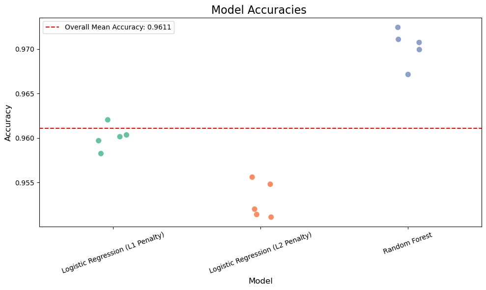
The aim of this was to evaluate multiple datasets comprising clinical and lifestyle variables to assess their predictive value for diabetes. This was done through building two different models that iterated through publicly available datasets, with numerous machine learning models such as Random Forest, Logistic Regression (L2 penalty), Logistic Regression (L1 penalty). We measured performance using accuracy on a held-out dataset. After multiple iterations, multiple accuracies for different models were obtained and plotted to compare and contrast with one another.

Across Dataset 1, the random forest classifier achieved the highest prediction accuracy of 97.003% (Figure 17), outperforming logistic regression models with both L2 (95.297%) and L1 (96%) penalties. The dummy classifier, included as a baseline for comparison, scored an accuracy of 91.667%. The dummy classifier in this instance was used to show contrast between models who actually take into account input data and predict and models who take simple rules and predict on the basis of those. Ex: predicting all values as true or false, or randomly basing your prediction based off of one variable, etc. The dummy classifier in dataset one has an accuracy of up to almost 91% which depicts a representation of how the data set is actually structured it shows how the data set is imbalanced and a simple method of predicting all false or all true in this case has a high percentage probability of predicting the actual value. In data set two this value is lowered showing how due to the boolean nature and the percentage of values being true against the whole dataset is greater in this case then with dataset 1 it is harder to predict using simple rules developed by the dummy classifier.

Evaluation on Dataset 1 demonstrated that accuracy alone overstated performance due to class imbalance, as the dummy classifier achieved a 91.667% accuracy. Incorporating additional metrics provided a more complete view showing that the dummy classifier achieved a recall and precision of 0.00 – depicting that it failed to identify any diabetes cases. The random forest model achieved the best results, with a precision of 0.96 indicating that most patients predicted as diabetic were indeed diabetic. While its recall of about 0.68 showed it correctly identified a majority of actual diabetic patients, its F1 score of 0.79 showed the highest balance and depicted it to be the most reliable model of all of them.

In contrast, models trained on Dataset 2, which consisted mostly of binary and categorical variables, achieved lower accuracy overall. Evaluation on dataset 2 revealed weaker model performance across all metrics compared to dataset 1. While logistic regression for L1 regularization achieved the highest accuracy at 84.65%, its precision (0.54) and recall (0.17) indicate a significant struggle in correctly identifying diabetic patients. This low recall means that the majority of diabetic cases were misclassified as non-diabetic, and the F1 score of 0.26 confirms the imbalance between precision and recall. Logistic regression with L2 regularization performed almost identically (accuracy 84.33%, F1 score 0.26), while the random forest model despite achieving the best recall among the three (0.19), only marginally improved the F1 score to 0.28 and produced the lowest ROC-AUC of 0.803, suggesting weaker discriminatory power. The dummy classifier once again highlighted the inadequacy of accuracy as a sole metric, recording an accuracy of 84.27% but failing entirely on precision, recall and F1 with an ROC-AUC of 0.5¹⁴.

In comparison to dataset 1, where Random forest achieved strong results (F1 score- 0.79, ROC-AUC – 0.964) and logistic regression L1 maintained a solid balance (F1 score – 0.72, ROC-AUC – 0.961), Dataset 2 demonstrates a substantial decline in both discrimination and robustness. The dramatic drop in recall (from ~0.60-0.68 in Dataset 1 to ~0.17-0.19 in Dataset 2) and corresponding fall in F1 scores shows that the model struggled to generalize when applied to the second dataset. This contrast highlights Dataset 2, which contained more categorical and binary features, posed a great challenge for all models, reinforcing the importance of incorporating multiple evaluation metrics rather than relying on accuracy alone.

The dummy classifier in this case performed at 84.274%, reinforcing that Dataset 2 was more balanced, and that basic heuristics alone were less effective in this context (Table 4).

Bootstrap Confidence Intervals

Confidence intervals indicated that performance estimates were highly stable across bootstrap samples. The random forest model consistently outperformed others, with its accuracy (0.971, 95% CI: 0.969-0.973) and F1 score (0.798, 95% CI: 0.785-0.810) showing narrow intervals, confirming robustness.

In contrast Dataset 2 produced wider intervals and lower F1 scores across all models. Logistic regression (L1) achieved accuracy of 0.846 (95% CI: 0.839-0.865), but its recall remained poor at 0.174 (95% CI: 0.167-0.181). These overlapping intervals highlight the difficulty of discriminating diabetic cases from categorical lifestyle data alone.

Model (Dataset)	Accuracy CI	Precision CI	Recall CI	F1 CI
RF (D1)	0.969–0.973	0.941–0.978	0.656–0.706	0.785–0.810
LR-L1 (D1)	0.958–0.962	0.857–0.903	0.576–0.624	0.697–0.743
RF (D2)	0.836–0.847	0.475–0.545	0.170–0.210	0.252–0.308
LR-L1 (D2)	0.839–0.865	0.505–0.575	0.167–0.181	0.233–0.287

The accuracies of data set 1 models in comparison to dataset 2 models as dataset 2 contains a huge problem. The problem lies within how the dataset is structured and what type of values it stores. In this case dataset 2 stores mostly its values in the form of binary data where either the person is a smoker or non smoker, or whether the person consumes fruits or doesn’t. The problem with this kind of data is that it doesn’t explore the extent to which people are consuming fruits or smoke or any other variable for that matter. Thus the lack of precise data creates a similarity between individuals and narrows the line between variables that actually affect diabetes or not, as an individual who smokes once a month may not have diabetes but may still be listed as a smoker with the person who smokes everyday, with this person having diabetes thus making it harder for models to predict.

Comparative Interpretation of Feature Importance Across Models

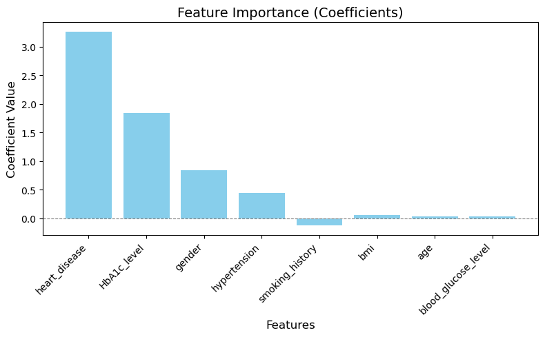
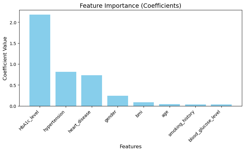
A major addition to the research was the addition of using a logistic regression model trained with an L1 penalty. An L1 penalty is when a logistic regression model weighs down certain variables with a negligible effect on the target variable to zero. This allows more emphasis on variables that play a significant role in determining whether the target variable is true or false thus being able to make a more accurate and precise prediction. However an L2 penalty is where these negligible factors aren’t weighed down to zero but are given a minimal value. In this research using an L1 penalty model did have a positive effect on the accuracy, being 96% in the first data set and 84.65% in the second data set showing a marginal improvement then when an L2 penalty for a logistic model was utilized. This shows how weighing down negligible factors allowed the logistic regression model to predict keeping into account only the main variables and it showed a higher precision in its prediction.

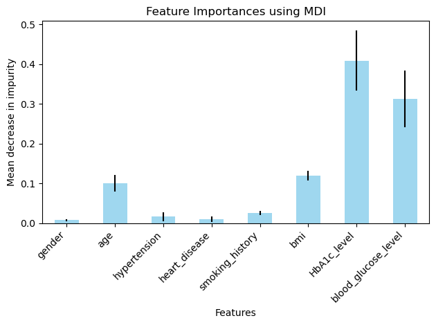
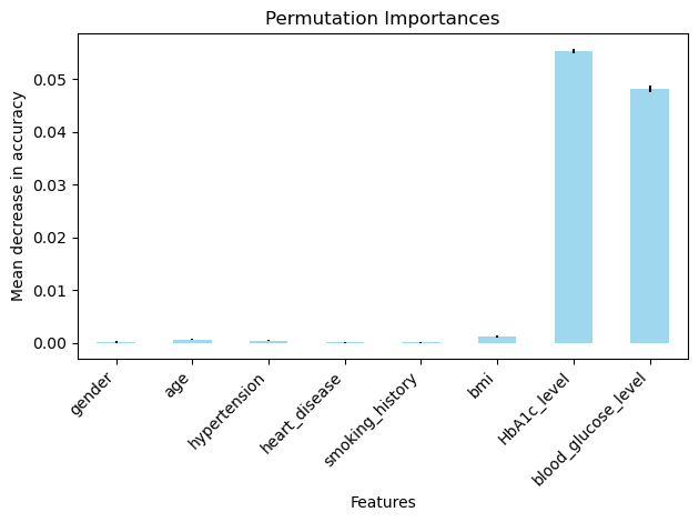
In the data set-1 the variables that affected the target variables the most were HBA1C level, whether or not the patient had heart disease, hypertension and their bmi (Figure 13-16). Although in this dataset that was unexpected to have this high of an impact on the final outcome which was gender (Figure 13). Even through prior research however we know that gender may not have any correlation to diabetes this dataset showed different results a possible explanation for this could be due to the size of the dataset or the dataset being skewed in such a way that there were more women with diabetes than women with non-diabetes and the opposite was true for the men in the dataset. This problem could be rectified by taking a more balanced and larger dataset, thus allowing us to explore the possibility of gender being an important correlate in the presence of diabetes.

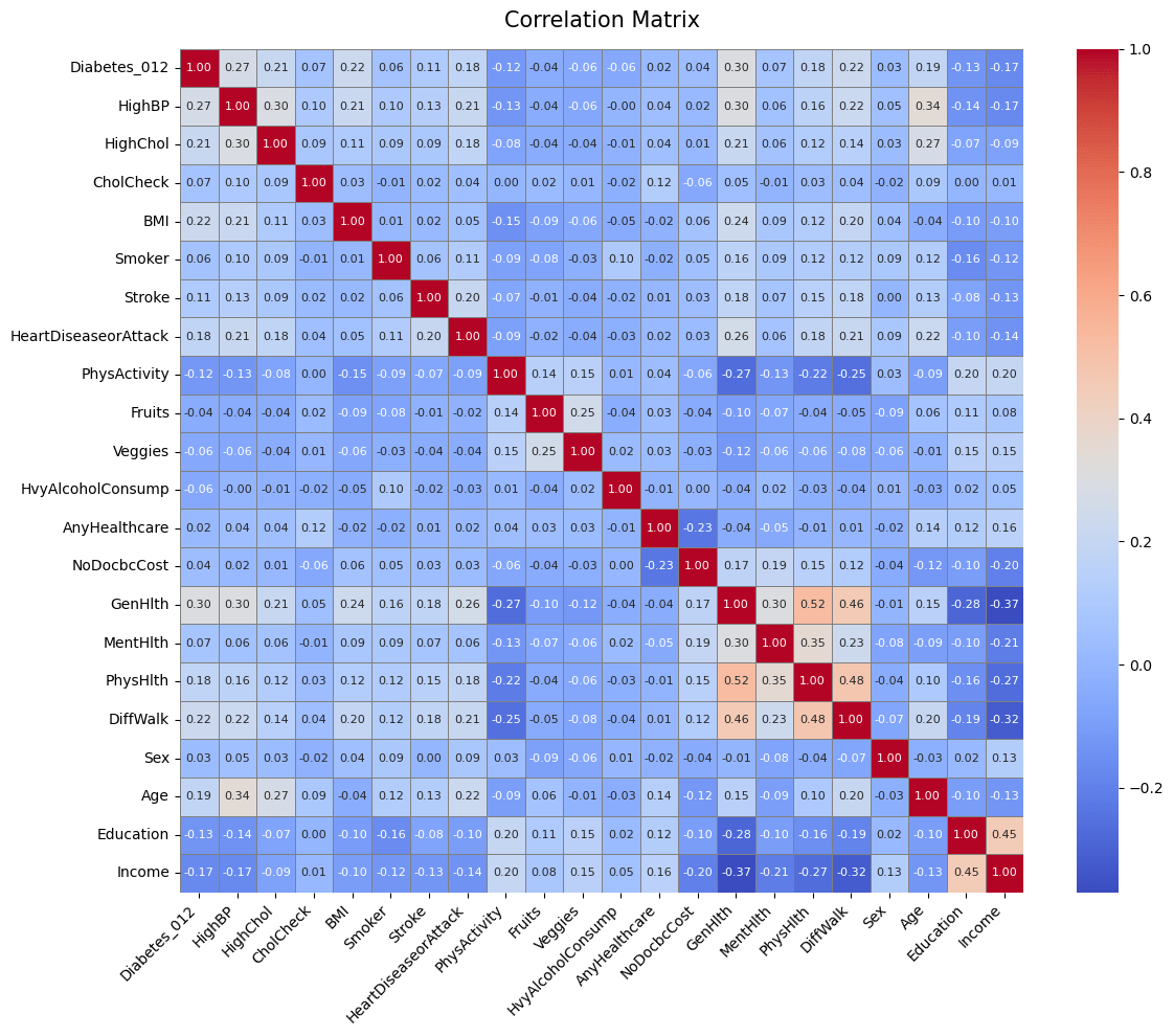
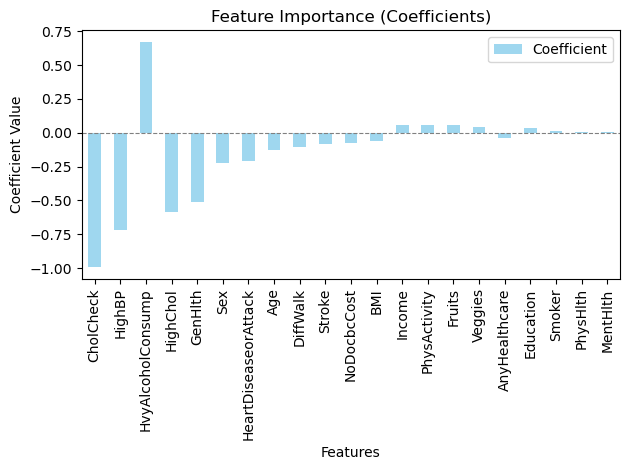
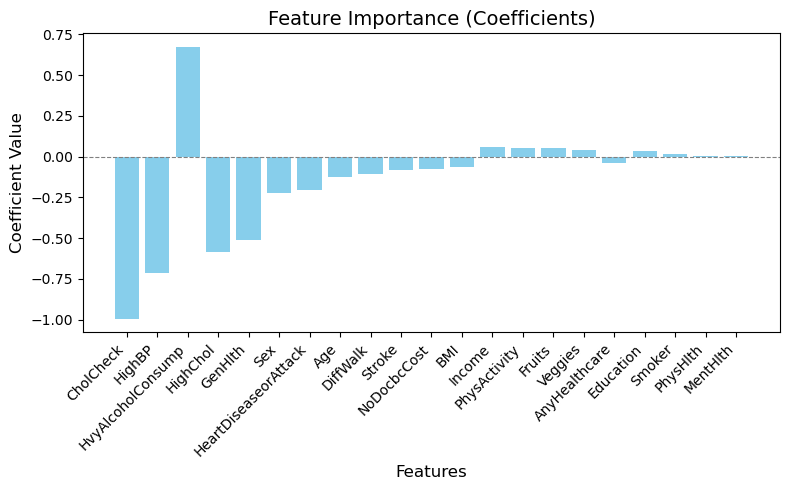
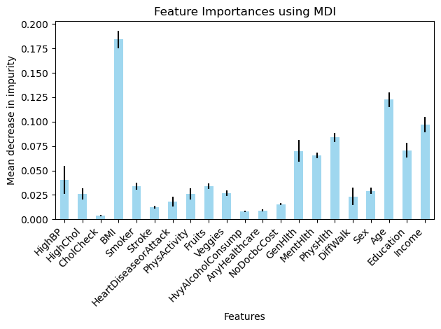
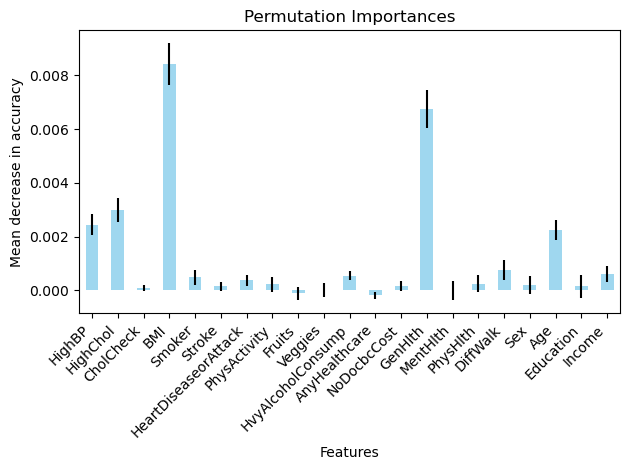
In data set 2 there were variables like alcohol consumption, BMI, generational health, Physical Health, age that had a larger impact on the presence of diabetes (Figure 22 – 25) although there were a few unexpected variables such as education, income, Mental Health (Figure 25) that also had an influence on the target variable. Again a possible explanation for this could be the size of the dataset and its imbalance with its nature of being a boolean dataset making it more difficult to determine a correlation between two variables.

Discussion

Dataset 1 contained few but more continuous variables, while dataset 2 comprised a large set of binary variables. Due to the distinct structuring of both datasets there were challenges while iterating through it to find the accuracies, for example due to the boolean type values in the second dataset, it was difficult for any machine learning model to identify key variables to predict whether the test sample had diabetes or not thus yielding a low accuracy and a varied feature importance graph which wasn’t optimal for this research.

Additionally, another key limitation amongst datasets was the class imbalance that existed within dataset 1. This may have inflated the predictive accuracy, as suggested by the high accuracy of the dummy classifier.

Similar studies conducted, for instance Nguyen and Zhang²¹ showcase a similar approach and their results showcase similar results with factors such as smoking, BMI, hypertension, etc. This study also emphasizes that even though Type-2 diabetes is predominantly affected by genetic factors, multiple lifestyle factors also shape the way on how severely diabetes can affect an individual. Febrian et al. similarly found that supervised machine learning models perform best when continuous clinical features are available²⁰. Tan et al.’s systematic review of machine learning methods for diabetes complications prediction further corroborates that model performance is heavily dependent on the quality and type of input features¹⁹.

The handling of missing values by encoding them as “no info” was another such limitation, which may have introduced noise into the models. Future studies should evaluate the usage of imputation techniques to improve predictive performance and reduce bias^17,18,22.

Also the exclusion of the “pre diabetes” individuals from data set-2 reduced the overall clinical applicability since pre-diabetes is an important stage for early prevention. Future work should consider predicting all 3 outcomes.

Because simple K fold validation was used rather than stratified cross-validation, some folds may have had imbalance class distributions thus influencing accuracy values in dataset 1. Stratified K fold validation should be employed in the future to ensure class proportions are preserved across folds.

For future improvements I would consider trying out ensemble methods as a strategy to yield higher accuracy values and more accurate feature importance graphs^11,15. Moreover, I would consider a hybrid approach to this research, where using feature engineering would be key to making a dataset suitable for this project. Lastly, I believe taking a boolean dataset was the wrong approach as the tradeoff between discrete, precise values for a range of variables wasn’t as suitable as I had presumed it would be.

Moreover, while model performance metrics were averaged across folds to ensure stability, feature importance values were reported from single model runs. This means the relative ranking of predictors may vary with different random seeds or cross validation splits, particularly for less influential variables. Future iterations of this work should address this by averaging importance scores across folds or by using permutations-based methods and reporting confidence intervals, to ensure that conclusions about the relative influence of the predictors remain robust.

Source code: https://github.com/AarushRaheja/Diabetes-Prediction-Model

References

1. E. Riveros Perez, B. Avella-Molano. Learning from the machine. BMJ Open, 2025. [↩]
2. M. Lugner et al. Identifying top ten predictors of type 2 diabetes. Scientific Reports, 2024. [↩]
3. M. Ravaut et al. Development and validation of a ML model using admin health data. JAMA Network Open, 2021. [↩]
4. Y. Qin et al. ML models for data-driven prediction of diabetes by lifestyle type. IJERPH, 2022. [↩]
5. K. J. Rani. Diabetes prediction using machine learning. IJSCSEIT, 2020. [↩]
6. M. J. Noh, Y. S. Kim. Diabetes prediction through causal discovery. Biomedicines, 2025. [↩]
7. F. Mohsen et al. A scoping review of AI-based methods for diabetes risk prediction. npj Digital Medicine, 2023. [↩]
8. H. Zhou, Y. Xin, S. Li. A diabetes prediction model based on Boruta feature selection. BMC Bioinformatics, 2023. [↩]
9. P. Negi. Evaluating feature selection methods for diabetes prediction with random forest. ACM, 2024. [↩]
10. A. A. Alhussan et al. Classification of diabetes using feature selection and hybrid optimization. Diagnostics, 2023. [↩]
11. I. Tasin et al. Diabetes prediction using ML and explainable AI techniques. Healthcare Technology Letters, 2023. [↩] [↩]
12. P. Rajendra, S. Latifi. Prediction of diabetes using logistic regression and ensemble techniques. CMPB Update, 2021. [↩] [↩]
13. Y. Edlitz, E. Segal. Prediction of T2DM onset using LR-based scorecards. eLife, 2022. [↩] [↩]
14. S. Wang. Diabetes prediction using random forest in healthcare. Highlights Sci. Eng. Technol., 2024. [↩] [↩]
15. A. Abousaber. Robust predictive framework for diabetes classification on imbalanced datasets. Frontiers in AI, 2024. [↩] [↩]
16. S. M. Ganie, M. B. Malik. An ensemble ML approach for predicting type-II diabetes. Healthcare Analytics, 2022. [↩]
17. S. W. J. Nijman et al. Missing data is poorly handled and reported in prediction model studies. J. Clin. Epidemiol., 2022. [↩] [↩] [↩]
18. M. Liu et al. Handling missing values in healthcare data. Artif. Intell. Med., 2023. [↩] [↩]
19. K. R. Tan et al. Evaluation of ML methods for prediction of diabetes complications. J. Diabetes Sci. Technol., 2023. [↩] [↩] [↩]
20. M. E. Febrian et al. Diabetes prediction using supervised machine learning. Procedia Computer Science, 2023. [↩] [↩]
21. B. Nguyen, Y. Zhang. A comparative study of diabetes prediction based on lifestyle factors. arXiv, 2025. [↩]
22. R. Rios et al. Handling missing values in ML to predict patient-specific risk. Comput. Biol. Med., 2022. [↩]