Practical Recommendations For Machine Learning-Based Tabular Regression Concerning Car Price Prediction

Abstract

Predicting car prices accurately is a significant problem in the automotive industry, influencing buyer and seller transactions. Due to the rising uncertainty of market dynamics and consumer preferences, accurate car price prediction is crucial in today’s market. In this paper, various machine learning and deep learning algorithms have been examined to predict car prices accurately. A dataset of used vehicles, including their details and listing prices, was utilized, and various preprocessing techniques were applied to enhance the data quality. Specifically, four imputation methods- that is, mode, mean, K-Nearest Neighbor imputation, and median- were employed to fill in missing values in the data. Further, feature engineering was done, splitting the name feature into brand and model names. Finally, various machine learning and deep learning models were employed to predict car prices based on the refined feature set. The hyperparameters of each deep learning model were adjusted to enhance its overall performance. It was observed that the feature engineering-enhanced approach improved the accuracy of most machine learning and deep learning models, demonstrating that careful data preprocessing and feature engineering (like splitting the car names) can enhance model performance. The impact of each feature was investigated and subsequently the mileage feature was dropped based on the three independent methods (SHAP, Permutation importance, and marginal non-linear dependency). LightGBM and CatBoost were identified as the best models based on their R² scores. These experiments prove that while deep learning offers powerful tools for complex machine learning problems, traditional machine learning models can sometimes provide better performance for tabular datasets, especially when feature engineering is effectively applied. Broadly, it highlights the importance of domain-specific preprocessing techniques in improving model accuracy.

Introduction and background

Accurate car price predictions are highly valued in a volatile car market, enabling consumers to make informed purchasing decisions. Knowing the approximate fair market value of a car (whether new or used) often helps consumers pay the right price for the vehicle. Having a fair idea of market trends also allows manufacturers and analysts to study and examine consumer preferences over both short-term and long-term periods. In a rapidly globalizing world, accurately estimating the right price is crucial to avoid under- or overpaying. Car dealerships and websites (like CarWale, TrueCar, or CarDekho) use price prediction models to set competitive prices and, therefore, attract prospective buyers. It helps them make healthy profits while keeping customers happy.

Moreover, the growth of the internet has dramatically increased the information available to potential buyers in multiple markets, significantly addressing the problem of adverse selection.

Given the rise of electric vehicles (EVs), fuel costs are changing, resulting in a corresponding shift in car prices. Supply chain issues, chip shortages, and inflation affect car prices worldwide, making machine learning-based price prediction a necessity rather than a choice.

Additionally, the second-hand car market is expanding, which is accompanied by a corresponding decline in the market for new cars. The price of both used and new cars depends on several factors, including fuel type, color, model, mileage, transmission type, engine type, number of seats, and brand value. Most people prefer to buy used cars because they generally tend to be affordable (about 50% cheaper than new cars) and can be resold again to get some profit. Hence, machine learning to predict car prices is becoming increasingly important. The research paper aims to explain how different machine and deep learning algorithms were leveraged to perform accurate car price prediction.

Related Works

Several studies and related works have been conducted in the past to predict car prices, as well as those of new cars worldwide, using various methods and approaches. In 2023, Researchers employed Linear Regression modeling for used car price prediction. They evaluated the model’s effectiveness in predicting prices¹.

Along similar lines, a study published in December 2019 utilized machine learning algorithms, including Lasso Regression, Multiple Regression, and Regression Trees, to develop a statistical model that predicted the price of a used car based on previous consumer data and a given set of features²

On the contrary, researchers in the United States used artificial neural network algorithms for the same purpose. They developed artificial neural network algorithms using the Keras regression algorithm and compared their performance to that of basic machine learning models, including Linear Regression, Decision Tree algorithms, Gradient Boosting, and Random Forest³.

Elsewhere, researchers proposed a supervised machine learning model using the K-Nearest Neighbor (KNN) regression algorithm to analyze the prices of used cars. They claim the accuracy of the proposed model to be around 85%. Although the paper’s aim was similar to the previous ones, i.e., to enhance model accuracy, it employed different techniques to achieve this goal: data preprocessing, including the removal of numerical components from non-numerical features, converting categorical values into numerical values, and separating the target variable⁴.

Furthermore, recent research has investigated the application of ensemble machine learning approaches for car price prediction using image-derived datasets⁵. The study leverages machine learning models and ensemble techniques to achieve an accuracy of 99.99%. Through testing and data pre-processing, the research demonstrates the importance of employing ensemble methods like bagging and stacking to improve model performance.

Similarly, in another study, researchers developed a car price prediction model for Bosnia and Herzegovina using data collected from a local car portal. Three machine learning techniques(ANN, SVM, and Random Forest) were applied in an ensemble to improve prediction accuracy. The final model was integrated into a Java application. It achieved an accuracy of 87.38%⁶.

This paper aims to address the problem of car price prediction primarily through the lens of feature engineering, including the removal and splitting of the various features present in the original dataset, as well as the use of different imputation methods. Moreover, it employs a vast array of machine learning models, from tree-based techniques to linear techniques to neural network-based models. Thus, it combines the previous efforts of researchers with a vast majority of the models in one paper.

This paper has two broad sections:

Materials and methods: A brief description of the dataset, followed by a similar in-detail description of how and why feature engineering was done. Lastly, this section provides a short explanation of the various machine learning and deep learning techniques used to accurately predict car prices, accompanied by diagrams to enhance clarity of understanding.

Experiments and Results: This section provides a concise overview of the implementation details, followed by a detailed explanation of how and why the machine learning and deep learning results were obtained.

This is followed by the conclusion.

Materials and Methods

Dataset description

The dataset consisted of twelve features, including the target variable.

The dataset used in this paper was sourced from CarDekho, one of India’s largest online platforms for buying and selling cars. It contains listings of second-hand vehicles across various regions of India. The outsourced dataset was taken from an open-source data science and machine learning community called Kaggle.

The twelve features are stated as follows:

1. Name- The full name of the car, including make, model, and variant. For example, “Maruti Swift Dzire VDI.” 
2. Year-The year of manufacture of the vehicle 
3. Kilometres driven (in kilometers)-Total distance the vehicle has been driven.
4. Fuel-Type of fuel used by the vehicle.
5. Seller type-the type of seller listing the car. For example, Individual or dealer.
6. Transmission- Indicates whether the car uses an automatic or manual gearbox.
7. Owner-Describes the number and type of previous owners.
8. Mileage (in kilometers per liter)- Fuel efficiency of the vehicle
9. Engine (in cubic centimeters)-Engine displacement of the car 
10. Maximum power(Horsepower or Brake Horsepower(BHP))-Maximum power output of the engine.
11. Seats-Total number of seats available in the car.
12. Selling price-target variable-The listed selling price of the car in Indian rupees.

The preprocessed dataset removed the mileage feature and split the name feature into brand and model.

There were 8128 samples for each feature. The split between the training and test data was 88% to 12%. Various aspects of the data were explored and diagrams plotted to gain a deeper understanding of it.

Pearson correlation coefficients between numerical and encoded variables in the dataset. The value of the coefficient can range from +1 to -1, representing the strength and direction of the linear relationship between the respective variables. A positive value denotes a positive correlation, a negative value denotes a negative correlation, and 0 indicates no correlation.

It was observed that the selling price has a strong positive correlation with maximum power (0.75), suggesting that vehicles with higher power tend to have higher selling prices. The value of the engine (0.45) indicates that vehicles with larger engine capacities tend to be priced higher. The year is (0.41), as newer models are usually more expensive. Maximum power is also strongly correlated with engine (0.70) and seats (0.19): power tends to increase with engine size and the number of seats, though the seat correlation is weaker. Kilometers driven show a weak negative correlation with selling price (-0.23), suggesting that higher mileage slightly reduces vehicle value. Mileage (km/liter/kg) is negatively correlated with engine size (-0.58), maximum power (-0.37), and the number of seats (-0.45), indicating that vehicle performance comes at the cost of fuel efficiency.

Categorical variables, such as fuel type, seller type, transmission, and ownership, were likely encoded for correlation analyses, as indicated by their low to moderate correlations with other variables.

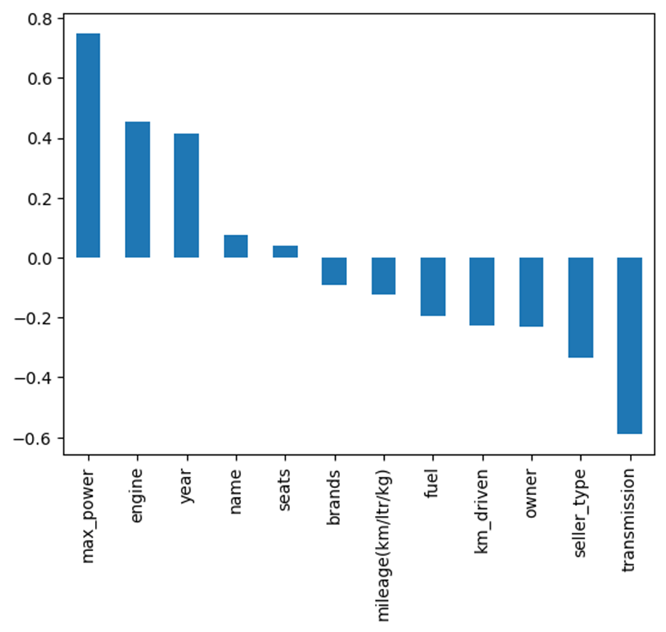
Strong Positive Correlations: Maximum power (~0.75): Cars with higher horsepower are typically priced higher. Engine (~0.45) and year (~0.41): Vehicles with larger engine capacities and newer manufacturing years tend to be highly priced.

Moderate Positive Correlations: Name and seats show minor positive relationships, possibly showing premium or larger vehicles such as SUVs, MUVs, or luxury vehicles.

Negative Correlations: Transmission (~ -0.55): Values likely indicate manual vs. automatic; manual is associated with lower prices. Seller type, owner, and km driven: Suggest that cars from certain sellers with more previous owners or higher mileage are priced lower. Mileage(km/liter/kg) (~ -0.20): This signifies that cars with higher mileage are often lower powered and hence cheaper.

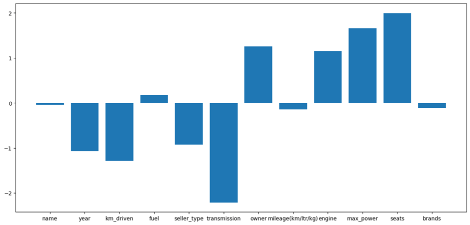
Positively Impactful Features: Seats, maximum power, and engine have the most significant positive coefficients, meaning they significantly increase the predicted selling price. Out of these, seats have the most decisive influence in this model, possibly due to being associated with luxury or premium cars. The owner and fuel also contribute positively to a lesser extent.

Negatively Impactful Features: transmission, kilometers driven, seller type, and year have negative coefficients, implying that these features lower the selling price in the model. For example, transmission likely represents a manual vs. automatic distinction, with manual vehicles being valued lower. Kilometers driven and year demonstrate depreciative factors, like vehicle usage and age.

Neutral Features: The coefficients for name, brands, and mileage (km/ltr/kg) are close to zero, indicating little to no influence on the model’s predictions.

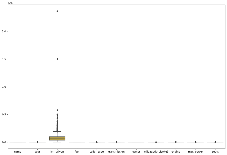
Kilometers driven: This feature displays a wide range of values, including several outliers, with extreme cases exceeding 2 million kilometers, which are likely erroneous. These outliers can skew model predictions and should be removed or changed. Most other variables show either minimal spread or are compressed near the lower end, suggesting their values are tightly clustered. Outliers exist in many variables (small dots above or below whiskers), but not to a great extent. The presence of such outliers can introduce a significant bias in the accuracy of various models.

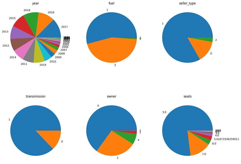
As shown in figure 5, the year distribution exhibits a wide range of car manufacturing years. However, most cars were produced between 2010 and 2018, with a few older vehicles (made before 2005) also present.

Fuel has been labeled numerically. Diesel and Petrol have the highest representation, with Petrol slightly more common. Electric and CNG vehicles are rare, suggesting limited alternative fuel options.  

Seller Type – The majority are labeled “1”, likely representing individual (solitary) sellers. Dealerships (possibly labeled “0” or “2”) make up a smaller portion.

Transmission – Many cars have a value of “1”, likely indicating a manual transmission. Automatic cars (value “0”) are much less frequent.

Owner- Most cars are first-hand (value 0), followed by second-hand (value 2). Vehicles with more than two owners (values 3 and 4) are rare, possibly due to reduced resale values and the pride associated with owning a car that is not a second or third-hand vehicle.

The dataset is dominated by 5-seater vehicles, which is standard for most sedans and hatchbacks. A small number of cars have 7 or 8 seats, suggesting SUVs or MUVs. Some unusual values (e.g., decimals like 5.41) may indicate data entry errors.

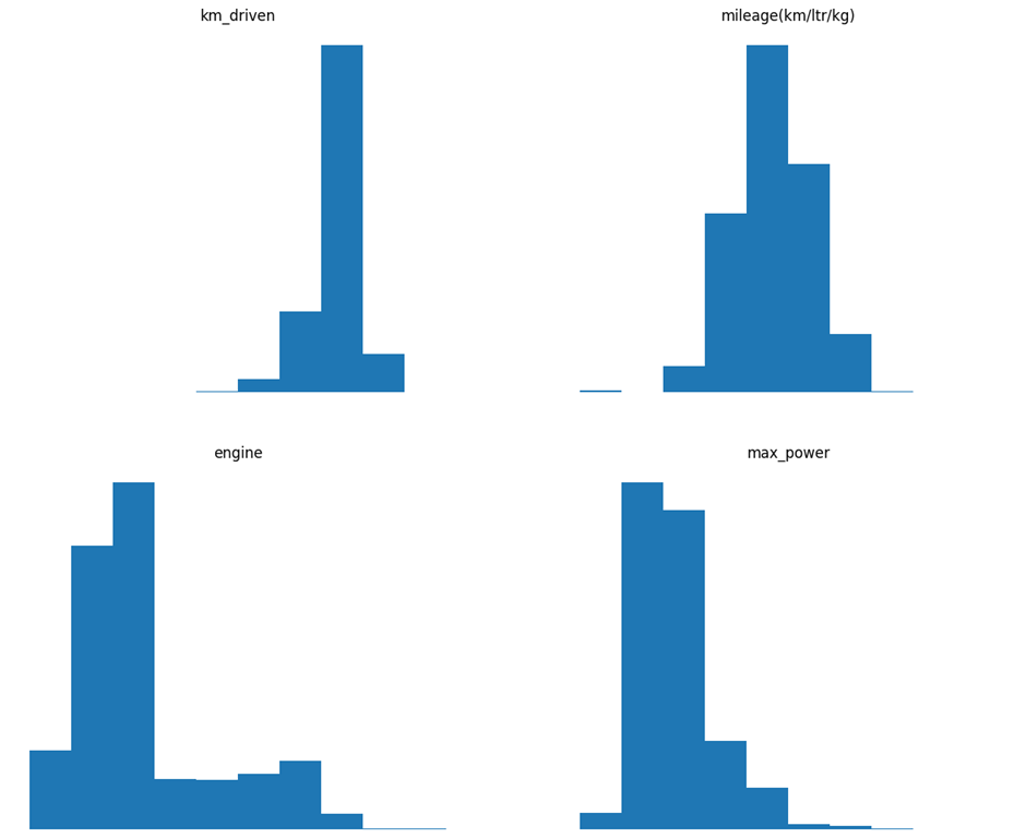
Kilometers driven- The distribution is right-skewed, with most cars driven under a specific limit (likely under 100,000 km) but a long tail of high-mileage vehicles. This result highlights the importance of handling outliers during preprocessing.

Mileage (km/ltr/kg) This variable is approximately normally distributed, centered around a typical fuel efficiency range (approximately 15–25 km/ltr).

Engine Skewed distribution toward lower engine capacities (standard for small, mid-size cars). Many observations are concentrated around the 1000–1500 cc (cubic centimeter) range, with fewer high-displacement engines.

Maximum power distribution is right-skewed, indicating that most cars possess average horsepower, with fewer high-performance exceptions.

Feature engineering

Missing value imputation

It was observed that four of the eleven features, namely mileage (km/ltr/kg), engine, maximum power, and seats, had some missing values.

The presence of missing data can significantly impact the performance and accuracy of machine learning algorithms. Specifically, missing data hinders model accuracy and performance because it can introduce bias, reduce the amount of available data, render some algorithms unusable, lead to the loss of valuable information, increase the complexity of the process, and compromise the stability of both machine learning models and deep learning models. To address this challenge, various imputation methods were explored to fill in missing values within the dataset. Previously, mean and mode were used to fill in numerical and string values, respectively. However, median and K-Nearest Neighbour imputation methods were also explored to determine if the change had any tangible impact on the models’ accuracy.

By choosing appropriate statistical measures (mean, median, mode, and KNN), the underlying distribution and variance of the data were preserved, thereby minimizing the distortion of the dataset.

These imputation techniques are efficient and easy to implement, making them suitable for handling large datasets with missing values.

Mean- The mean is the average value calculated by summing up all the available values and dividing by the total number of observations. Filling missing values with the mean is a straightforward method for estimating unknown values based on existing data⁷.

The median is the middle value in a dataset that has been sorted in ascending order. It represents the central tendency and is less sensitive to outliers compared to the mean.

Mode is the most frequently occurring value of the non-missing data for a specific variable.

KNN Imputation- It works by finding the “nearest neighbors” (rows) that have similar patterns to the row with missing data. In KNN imputation, each row is treated as a coordinate in a multi-dimensional space (each feature represents a dimension). The algorithm then calculates the distance between rows to identify the most similar ones. The missing value is then estimated based on the values of the closest rows⁸.

Decoupling brand and model name

To enhance the predictive accuracy of car prices, strategic feature engineering techniques were employed. In the original dataset, the car names feature contained redundant and overlapping information. For example, in the Skoda Rapid 1.5 TDI Ambition, the 1.5 represents the engine capacity, while the TDI represents the type of transmission used in the car. These features were already present as separate independent features in the dataset and, hence, were considered redundant. Moreover, the brand value was unaccounted for: two cars with the exact specifications and different brands will be priced differently, owing to distinct brand values. The name feature was split into two features: brand and model. This split enhanced the ability of models to independently assess the impact of specific brands and models on car prices. The improved feature independence and distinct representation of brand value significantly reduced the redundancy of the features, thus preventing multicollinearity.

Dropping mileage

Although initial correlation analysis showed a moderate negative correlation between mileage and maximum power (–0.37) and a weaker correlation with price (–0.20), a more thorough feature importance evaluation was conducted using three independent methods:

Using SHAP values, mileage ranked among the lowest features, contributing less than 2% of the total model importance. Moreover, randomly shuffling mileage resulted in negligible changes in the model’s accuracy (<0.5% change in MAE), indicating low predictive prowess(permutation importance). Finally, the mutual information score for mileage was close to zero(0.02), confirming marginal non-linear dependency with the target variable.

These results suggest that mileage’s role in the correlation features is largely indirect. Its inclusion neither improved nor stabilized the model’s performance. However, it slightly increased feature redundancy, as a result of which the mileage was dropped.

Machine learning techniques

‘Linear Regression model’- Such models assume a linear relationship between features and the target variable. Linear Regression is a type of supervised machine learning algorithm that learns from labeled datasets and maps the data points using the most optimized linear functions, which can then be used for prediction on new datasets. Specifically, it fits a straight line to the observed data by minimizing the mean squared error between the predicted and actual values. Finally, it predicts the continuous output variables based on the independent input variable.

‘Ridge Regression model’- Ridge Regression is a model-tuning method that is used to analyze any data that is affected by multicollinearity. This method employs L2 regularization. When the issue of multicollinearity arises, least-squares estimators are unbiased, but the variances are significant, resulting in predicted values that deviate substantially from the actual values.

The cost function for Ridge Regression is as follows

   

‘Lasso Regression model’- In Lasso Regression, the hyperparameter lambda (), also known as the L1 penalty, is used to balance the potential trade-off between bias and variance in the resulting coefficients. As increases, the bias increases, and the variance decreases, leading to a simpler model with fewer parameters. This is illustrated in the diagram below.

‘Elastic Net Regression model’- It is a Linear Regression algorithm that adds two penalty terms to the standard least-squares objective function. These two penalty terms are, namely- the L1 and L2 norms of the coefficient vector. These two terms are multiplied by the two hyperparameters, alpha and lambda. While the L1 norm is used to perform feature selection, the L2 norm’s primary function is feature shrinkage. The Elastic Net Regression model can be represented as follows:

   

Where y is the dependent variable, is the intercept, to are the regression coefficients, to are the independent variables, and e is the error term.

Decision Tree model- Decision Tree model- Decision Trees (DTs) are a non-parametric supervised learning method used for classification and regression tasks. This model predicts the value of a target variable by learning simple decision rules inferred from the data features. A tree can be seen as a piecewise constant approximation, as illustrated in the figure below.

‘Gradient Boosting model’- Gradient boosting is a machine learning technique that combines multiple weak prediction models into a single ensemble, as seen in the figure below. These weak models are typically decision trees, which are trained sequentially to minimize errors and improve accuracy. By combining multiple decision tree regressors or decision tree classifiers, gradient boosting can effectively capture complex relationships between features.

‘K-Nearest Neighbour model’- The K-Nearest Neighbour (KNN) algorithm is a non-parametric, supervised learning classifier that uses proximity to make classifications or predictions about the grouping of an individual data point.

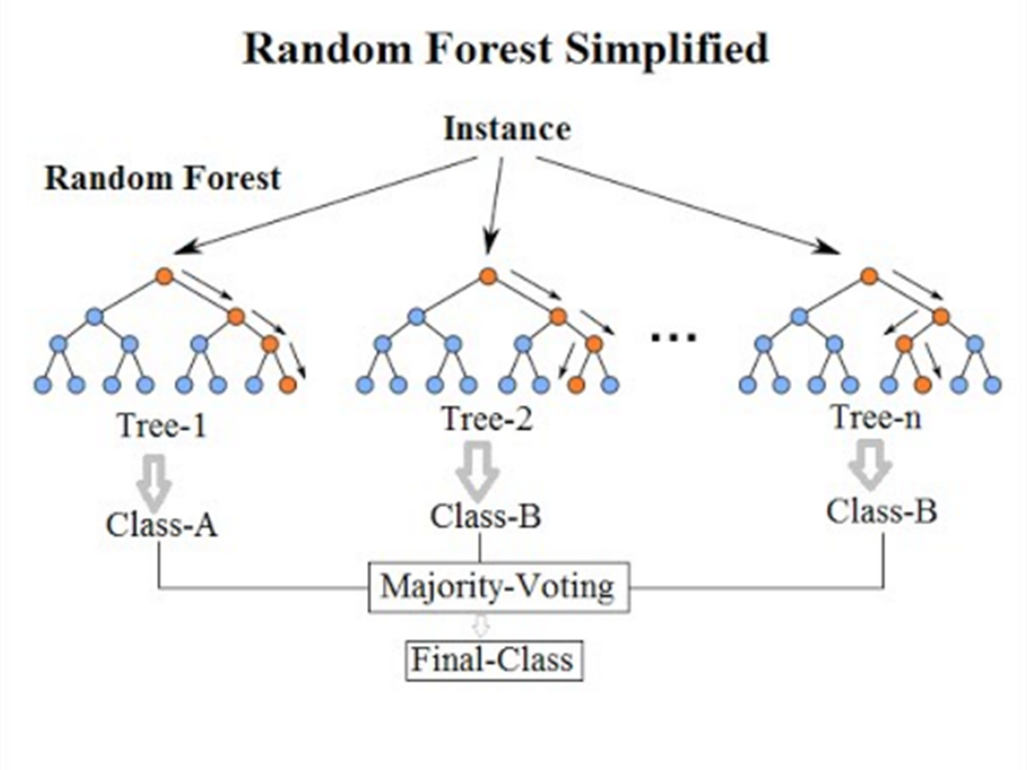
‘Random Forest model’- Random Forest algorithms have three primary hyperparameters, which need to be set before training. These include node size, the number of trees, and the number of features sampled. From there, the Random Forest classifier is used to solve regression or classification problems.

The Random Forest algorithm consists of a collection of Decision Trees, and each tree in the ensemble is comprised of a data sample drawn from a training set with replacement, known as the bootstrap sample. Of that training sample, one-third of it is set aside as test data, known as the out-of-bag (OOB) sample. Another instance of randomness is then introduced through feature bagging, which adds more diversity to the dataset and reduces the correlation among Decision Trees. Depending on the type of problem, the determination of the prediction will vary. For a regression task, the individual Decision Trees will be averaged, and for a classification task, a majority vote—i.e., the most frequent categorical variable—will yield the predicted class. Finally, the OOB sample is then used for cross-validation, finalizing that prediction. This is illustrated in the diagram below.

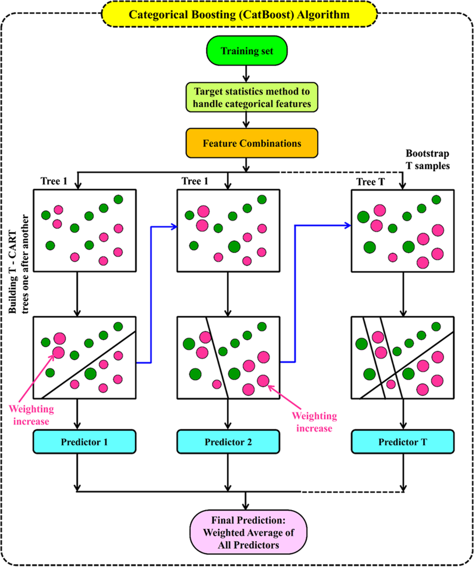
‘CatBoost’- CatBoost is built on the Gradient Boosting framework, an ensemble learning technique that combines the strengths of multiple weak learners to produce a predictive model. CatBoost implements this framework using Decision Trees, but what sets it apart are two critical innovations, namely ordered boosting and efficient handling of categorical features.

Ordered boosting is a technique that creates several permutations of the data and uses only past observations for each permutation when calculating leaf values. This method minimizes overfitting. While most gradient-boosting algorithms require these features to be converted into numerical representations through methods like one-hot encoding, CatBoost natively handles categorical data. It automatically determines the best way to represent these features, significantly reducing the need for manual preprocessing. It works exceptionally well when dealing with high-cardinality features. This generally happens when a feature has a considerable number of distinct values.

‘XGBoost’- XGBoost, which stands for Extreme Gradient Boosting, is a scalable, distributed gradient-boosted Decision Tree (GBDT) machine learning library with sequential ensemble learning. It is a supervised learning algorithm that handles missing values by default and is not sensitive to outliers. It provides parallel tree boosting and is the leading machine-learning library for Regression, classification, and ranking problems.

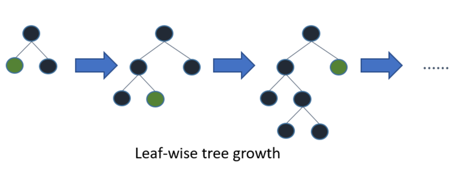
‘LightGBM’- The Light Gradient Boosting [6] machine regressor (LightGBM) is a breakthrough tree-based ensemble learning approach developed by researchers to overcome the efficiency and scalability difficulties of XGBoost in high-dimensional input features and massive dataset contexts. The LightGBM technique comprises two primary methods: exclusive feature bundling (EFB) and gradient-based one-side sampling (GOSS), both of which are based on Decision Trees. As with other Decision Tree-based methods, LightGBM can be used for both classification and Regression. It is optimized for high performance with distributed systems. LightGBM creates Decision Trees that grow leaf-wise, which means that given a condition, only a single leaf is split, depending on the gain. Leaf-wise trees can sometimes overfit, especially with smaller datasets. Limiting the tree depth can help to avoid overfitting.

Deep learning techniques

Artificial Neural Networks and What They Are About – Artificial neural networks contain artificial neurons called units. Together constituting the whole Artificial Neural Network in a system, these units are arranged in a series of layers. A layer can have only a dozen units or millions of units, as this depends on the complexity of the neural networks required to learn the hidden patterns in the dataset.

More commonly, an Artificial Neural Network consists of an input layer, an output layer, and one or more hidden layers. The input layer receives data from the outside world, which the neural network needs to analyze or learn about. Thereafter, this data passes through one or more hidden layers, transforming the input into data that is valuable for the output layer. Finally, the output layer provides an output in the form of a response of the Artificial Neural Networks to the input data provided.

Sequential models were constructed using fully connected layers. The number of layers and units per layer were kept consistent across initial experiments to allow for fair comparisons.

Rectified Linear Unit (ReLU) activation functions were used for hidden layers to introduce non-linearity. A linear activation function was used for the output layer to allow for continuous value predictions.

Experiments and results

Implementation details

Out of 8128 samples in the dataset, it was found that 221 samples were missing in each of the three features —mileage, seats, and engine. For maximum power, the number of missing samples was 215. This led us to employ the various missing value imputation techniques.

	Mean value	Median value
Mileage	19.418783	19.418783
Engine	1458.625016	1248.000000
Seats	5.416719	5.000000

The mode value for the maximum power was found to be 74.0

For the KNN imputation method, the number of nearest neighbors used was five, with uniform weights.

To maintain consistency and comparability across models, the default hyperparameter settings as prescribed by the respective Python packages for each machine learning model were used. Scikit learn was used to implement these algorithms(machine learning models).

All experiments were conducted with a fixed random seed (42) for reproducibility.  Key packages and their versions: Scikit-learn 1.X, Keras 2.X, TensorFlow 2.X, NumPy 1.X, Pandas 1.X, Matplotlib 3.X.

Several deep-learning models were employed with different hyperparameters and layers. Keras was used as the default framework. All the sequential models took the same input as the machine learning models, which were trained and tested. No normalization layers were used in the model. The Adam optimizer was chosen for its adaptive learning rate capabilities, with default parameters (learning rate = 0.001, beta_1 = 0.9, beta_2 = 0.999, epsilon = None, decay = 0.0). Mean Squared Error (MSE) was used as the loss function to quantify the difference between predicted and actual values. The R-squared (R²) score was used to evaluate the model’s performance. A batch size of 32 was used. Models were trained for a maximum of 1000 epochs with an early stopping callback to prevent overfitting. The early stopping monitored validation loss and stopped training if no improvement was observed for 50 epochs. Dropout layers with a rate of 0.1 or 0.2 were added to some models to prevent overfitting.

Three models with different layers in deep learning:

Model 1 was a neural network model with configurations of 16, 8, and 4 neural network units in the hidden layer. Use of default activation function for output “Relu .” Model 2 was a neural network model with configurations of 64, 64, 128, 128, and 256 neural network units in the hidden layer. A dropout rate of 0.1 was included, which was used to regularize the output from hidden layers 4, 5, and 6, which fed into the output layer.

A linear activation function was used for the output, which is more appropriate for Regression.

Model 3 was a neural network model with configurations of 128, 128, 256, 256, and 512 artificial neural network (ANN) units in the hidden layer. A dropout rate of 0.2 was included, which was used to regularize the output from hidden layers 4, 5, and 6, which fed into the output layer.

A linear activation function was used for the output, which is more appropriate for Regression.

Feature engineering results

The results, which depict the impact of feature engineering, are shown below.

The results are displayed in two features: one with the impact of feature engineering (after dropping mileage and decoupling) and the other without this impact. 

Models	Test R2 score (%)	Test R2 score (%)
	without feature engineering	with feature engineering
Linear Regression	63.15	63.28
XGBoost	94.63	95.84
CatBoost	96.13Table 2: Results of feature engineering	96.11
LightGBM	96.37	96.52
Lasso Regression	63.15	63.28
Ridge Regression	63.16	63.28
Elastic Net Regression	62.93	63.06
Decision Tree	86.82	90.69
Gradient Boosting	93.35	94.02
K- Nearest Neighbors	86.54	86.58
Random Forest	95.69	95.82

Table 2 shows that Linear Regression improved by 0.13%. A small gain from reduced redundancy, that is, decoupling brand and model slightly reduced multicollinearity, and mileage removal helped remove unnecessary noise.

XGBoost improved by 1.21%. Decoupling enhanced the model’s ability to distinguish between brand-level pricing (the brand value) and dropping mileage reduced overfitting.

CatBoost dropped by 0.02%. A minimal decline due to CatBoost’s inherent handling of high-cardinality categorical data such as the one used in this dataset

As seen in table 2, LightGBM improved by 0.15%. Categorical splits benefited from decoupling, and removing a relatively weekly correlated variable, such as mileage, led to a more focused approach.

Lasso Regression improved by 0.13%. This model benefited slightly from the reduction of multicollinearity and the elimination of the redundant mileage feature.

Ridge Regression improved by 0.12%. It gained in performance due to increased feature independence(by decoupling) and noise reduction from mileage removal.

Elastic Net Regression- Improved by 0.13%. Combined regularization performed better in the simplified feature space after decoupling, resulting in a decrease in mileage.

As illustrated in table 2, Decision Tree improved by 3.87%. A significant gain from more precise decision boundaries enabled by brand/model split and removal of redundant mileage feature.

Gradient Boosting- Improved by 0.67%. Better feature clarity(after decoupling) led to improved splits, especially with brand-based pricing distinctions.

KNN- Improved by 0.04%. There was slight improvement due to better distance calculations after eliminating irrelevant mileage and clarifying categorical data.

Random Forest- Improved by 0.13%. It gained marginally from cleaner data splits and a reduction in confusion caused by mileage drops.

Hence, table 2 displays succinctly how all models except CatBoost showed an improvement in model performance after feature engineering, demonstrating the need for careful preprocessing in conjunction with model specifications and behavior.

Imputation methods

Models	Test R2 score without imputation methods, where all missing values have default value zero(%)	Test R2 score for mean(%)	Test R2 score for median(%)	Test R2 score for KNN Imputation method(%)
Linear Regression	61.73	63.28	63.30	63.28
XGBoost	96.76	95.84	95.72	95.84
CatBoost	96.15	96.11	96.25	96.11
LightGBM	96.30	96.52	96.45	96.52
Lasso Regression	61.73	63.28	63.30	63.28
Ridge Regression	61.73	63.28	63.30	63.28
Elastic Net Regression	61.29	63.06	63.08	63.06
Decision Tree	88.11	90.69	91.66	93.13
Gradient Boosting	94.06	94.02	94.22	94.07
K-Nearest Neighbour	86.57	86.58	86.58	86.58
Random Forest	96.04	95.83	96.20	95.90

Linear Regression is sensitive to missing values, and hence, it is seen that there is an approximately 1.55% percent increase with the use of imputation methods. This is because the placing of default zero values introduces bias and affects coefficients. Mean, median, and KNN all remove this bias similarly, leading to nearly identical performance (with very little disparity).

XGBoost is inherently designed to handle missing values efficiently by learning split directions. Imputation slightly reduces performance, suggesting the model’s missing handling is better than imposed imputations in this case. Mean and KNN are tied(95.84%), and the median is slightly worse(95.72%).

As seen in table 3, CatBoost, like XGBoost, handles missing values implicitly. All imputation methods result in nearly equal performance(96.11 to 96.25%). Median performs better due to its resistance to outliers.

LightGBM showed a test R² score of 96.30% without imputation. However, the mean showed a minor improvement at 96.52%, and the median was 96.45%, with KNN also achieving an accuracy of 96.52%. There was a small gap of 0.07% between the R² scores with and without imputation methods. Therefore, these results show that LightGBM benefits slightly from imputation. Mean and KNN are tied, and the median is slightly behind. Nevertheless, all three are very close, indicating the inherent robustness of the model.

Lasso Regression without imputation stood at an R² score of 61.73%. However, the performance of the different imputation methods is not significantly different from one another: the mean yields an R² score of 63.28%, the median 63.30%, and KNN also achieves 63.28%. Lasso (being a linear model with L1 regularization) shares the same imputation insensitivity as Linear Regression.

Our results in Table 3 show that Ridge Regression shows no meaningful change in R² score values when different imputation methods are applied. Like Lasso, Ridge is a linear model with L2 regularization. It shows consistent behavior with very similar performance across imputation methods.

Elastic Net Regression also shows a negligible change in the R² score when different imputation methods are used. This is because it is a combination of Lasso and Ridge, and thus, Elastic Net Regression behaves similarly to the other two models. Moreover, there is an improvement of approximately 1.8% over the default zero imputation, as seen in Table 3.

The Decision Tree Model, with an R² score of 88.11% and default zero values, shows a significant difference of ~5% compared to KNN at 93.13%. The disparity between the mean and median is relatively intangible. Decision Trees split on feature thresholds. However, zeros skew these splits. Therefore, the reduced performance is seen, as displayed in Table 3. On the other hand, KNN captures more nuanced patterns, thereby improving the quality of splits. The model shows the highest gain from imputation among all models.

Gradient Boosting is a strong model with internal robustness. Hence, all imputation methods perform similarly. The median performs better than the other two imputation methods, as seen in Table 3.

K Nearest Neighbours Model shows the same R² score across all columns. This is because KNN classification bases predictions on similarity. Missing values imputed any which way lead to stable neighbor sets being formed. The results demonstrate that the KNN model is inherently robust and unaffected by the imputation strategy, as applied to this dataset.

Random Forest has some inbuilt tolerance to missing values. Hence, default zero imputation gives a slightly higher value as compared to the imputation methods. Overall, all imputation methods give close results. Median imputation marginally outperforms the rest.

Most models show no meaningful difference in performance between mean, median, and KNN imputation because the dataset has a low quantity of missing values as compared to the sample size.

Since our data was already preprocessed, changing the imputation methods had no tangible impact on the target variable and the accuracy of the models, as illustrated by table 3. Moreover, this was because “seats” and “mileage” were relatively independent of other critical features and had minimal impact on the target variable.

Machine learning results

Models	Test R2 score(%)	Train R2 score(%)	test mean squared error(x 1010 INR2 )	train mean squared error ( x 109 INR2)	test mean absolute error(x 104 INR)	train mean absolute error(x 104 INR)
Linear Regression	63.28	69.33	20.4	203	29.17	27.77
XGBoost	95.84	99.54	2.31	3.02	7.461	3.835
CatBoost	96.11	99.22	2.16	5.19	7.568	4.982
LightGBM	96.52	98.34	1.94	11	7.724	5.715
Lasso Regression	63.28	69.33	20.4	203	29.17	27.77
Ridge Regression	63.28	69.33	20.4	203	29.17	27.77
Elastic Net Regression	63.06	66.36	20.5	223	28.51	28.13
Decision Tree	93.03	99.96	3.88	0.291	9.223	0.4351
Gradient Boosting	94.10	97.57	3.28	16.1	9.840	7.884
KNN	86.58	94.77	7.46	34.6	10.75	6.773
Random Forest	95.84	99.50	2.31	3.33	7.783	2.611

Note: MAE (Mean Absolute Error) measures the average absolute deviation between predicted and actual prices. It is expressed in INR, i.e, in the same units as the target. MSE (Mean Squared Error) is a squared error metric which penalizes larger deviations more heavily. It is expressed in INR², making it less interpretable for direct use.

Linear Models (Linear, Lasso, Ridge, Elastic Net) show poor performance on average (test R² score around 63%). This is because these models assume linear relationships between the features and the target. Therefore, they fail to capture interactions between different features (e.g., year and transmission affecting price together). Lasso and Ridge attempt regularization, but they still inherit linear assumptions. ElasticNet combines both but remains limited when modeling complex real-world data, such as used or new car prices, as used in this dataset. Hence, these models tend to underfit the data.

Table 4 illustrates that tree-based models (Decision Tree, Random Forest, XGBoost, LightGBM, and Gradient Boosting) demonstrated excellent performance on average, with test R² scores ranging from 90% to 96%. This is because these models handle non-linearity naturally — perfect for real-world price fluctuations. Additionally, they split the data in order, identifying thresholds such as Year > 2015 or Fuel = Diesel, which affect car prices. Random Forest is an ensemble of Decision Trees, thus naturally reducing overfitting and improving stability. Both XGBoost and LightGBM are examples of Boosted trees, which will enhance performance by correcting previous tree errors, thereby resulting in better generalization.

As seen in table 4, LightGBM provided the best accuracy with a test R² score of 96.52%.

Gradient Boosting is also very similar in logic, as it uses sequential learning to achieve strong performance on structured data.

CatBoost slightly decreased (96.13% → 96.11%) after feature engineering, although it remained the second-best model with an R² score of 96.11%. This is because CatBoost is designed explicitly for datasets with numerous categorical variables. It efficiently encodes categorical features internally and performs well without requiring the preprocessing of categorical data, unlike most other models used in this paper. Hence, CatBoost showed an overall strong performance but dropped slightly after feature engineering due to interference from manual preprocessing (feature engineering made it redundant and somewhat noisy).

K-Nearest Neighbour (KNN) demonstrated a moderate performance, achieving a test R² score of 86.8%, as illustrated in table 4. This is because the model is instance-based, learning from existing data points by comparing new inputs based on “distance.” It is highly responsive to scaling and the numerical encoding of features. Moreover, this model struggles when data has high dimensionality or when categorical values aren’t well-represented numerically (as was the case with some of the features in this dataset).

Additionally, a dataset of 8128 samples is insufficient for high-capacity models to generalize well. This has a significant negative impact, as seen in the table above, with substantial differences in train and test R² scores. While linear models exhibit minor differences, they underfit due to their limited expressive power. Increasing sample size in general and proving coherence between features (categorical values represented well numerically) would reduce overfitting, improve test accuracy, and narrow the train-test R² gap.

Predictive performance of LightGBM by car manufacturer

Brand	Samples	MAE (₹)	RMSE (₹)	R²(in %)
Lexus	2	8,537.86	8,537.86	0
Jaguar	3	11,953.30	19,636.97	99.27%
Maruti	286	46,655.96	67,166.15	91.59%
Hyundai	171	57,042.38	81,435.24	91.97%
Tata	86	58,125.94	84,049.24	93.71%
Fiat	6	65,517.48	89,460.41	45.62%
Ford	55	68,698.69	101,833.57	89.95%
Datsun	6	71,440.85	89,640.26	44.84%
Skoda	16	74,690.09	119,554.58	96.15%
Renault	37	74,764.33	113,444.84	83.12%
Nissan	6	85,803.58	112,056.05	86.51%
Mahindra	66	90,682.30	120,967.98	80.18%
Volkswagen	31	91,223.94	132,255.76	70.56%
Honda	71	93,211.54	131,098.58	85.35%
Chevrolet	36	112,392.74	254,832.82	-1.39%
Toyota	50	116,149.24	166,087.47	92.68%
Isuzu	2	144,313.37	179,622.31	-1493.29%
Mitsubishi	4	149,315.03	196,613.92	87.22%
Jeep	4	183,351.07	250,636.38	94.29%
BMW	11	217,019.38	318,793.21	97.07%
Audi	9	253,528.25	322,718.64	83.00%
Mercedes-Benz	10	383,611.32	523,134.73	87.15%
Volvo	4	503,574.63	786,376.66	61.71%

As seen in table 5, the best Performing Brands are Jaguar, Maruti, Hyundai, Tata. This is because they have low MAE (<₹60K) and high R² (>0.91). These brands have ample samples and relatively consistent pricing, which helps LightGBM learn their price patterns effectively.

Moderately Performing Brands are Ford, Mahindra, Honda, Renault. They have a moderate MAE (₹68K–₹93K) with good R² (0.80–0.90), because these brands may have slightly higher price variability.

Poorly Performing Brands such as Isuzu, Volvo, Mercedes-Benz, Audi have very high MAE (>₹2.5L) and in some cases negative R². This indicates a poor fit, the common causes for which include very few training samples (≤10) and wide price ranges.

Therefore, it can be concluded that performance strongly correlates with sample size and price stability within each brand. LightGBM excels with popular, mid-priced brands but struggles with rare or luxury brands, mainly because of limited data.

Testing of LightGBM on unseen data, generalising to new categories

On the unseen brand test, LightGBM performance dropped sharply. This is because MAE ≈ ₹6.94 L, RMSE ≈ ₹8.87 L, and R² ≈ 0.617. This indicates poor generalization when predicting brands are not present in training.

In contrast, for unseen model combinations, performance remained strong, that is, MAE ≈ ₹44.15 K, RMSE ≈ ₹61.03 K, and R² ≈ 0.956. This shows how the model can generalize well to new models within known brands but struggles with entirely new manufacturers.

Comparison of models based on statistical tests

Model	Mean R²(%)	Standard Deviation	95% Confidence Interval
Linear Regression	68.00%	0.027	[0.647, 0.713]
XGBoost	96.50%	0.008	[0.955, 0.975]
CatBoost	96.40%	0.015	[0.945, 0.982]
LightGBM	96.60%	0.009	[0.954, 0.977]
Lasso Regression	68.00%	0.027	[0.647, 0.713]
Ridge Regression	68.00%	0.027	[0.647, 0.713]
Elastic Net Regression	65.10%	0.030	[0.614, 0.688]
Decision Tree	94.30%	0.016	[0.922, 0.963]
Gradient Boosting	95.30%	0.013	[0.937, 0.969]
KNN	89.10%	0.042	[0.838, 0.944]
Random Forest	96.40%	0.006	[0.956, 0.972]

The 95% confidence interval gives a range within which the true meanperformance of the model likely falls, with 95% confidence. A narrow CI generally means that there is more certainty while predicting the mean value.  

Tree-Based Ensemble Models

These models achieved the highest R² scores (≈0.95–0.97) with low standard deviations and narrow confidence intervals, indicating they consistently captured the complex, nonlinear relationships in the data with maximum precision. They are robust to feature scaling and can handle both linear and nonlinear patterns. 

Table 6 shows that Random Forest and Gradient Boosting also performed very well, but the boosting algorithms (XGBoost, CatBoost, LightGBM) slightly performed better in average performance.

Decision tree

As seen in table 6, Decision Tree model performed quite well (**R² ≈ 0.94**), but not as high as the ensemble tree-based models. While it can capture nonlinearity, it is more prone to overfitting and less stable across data splits, as reflected by its slightly higher standard deviation and wider confidence interval.

Linear Models

These models had moderate R² scores (≈0.65–0.68), indicating that linear relationships capture less of the variance in the data. Lasso and Ridge performed almost identically to linear regression, suggesting regularization did not bring significant improvement. Elastic Net performed slightly worse, perhaps due to the balance of L1 and L2 penalties not being optimal for this dataset.

Overall, as seen in table 6, linear models are less able to capture complex interactions present in your data compared to tree-based models.

KNN (K-Nearest Neighbors)

As illustrated in table 6, KNN achieved an R² score (≈0.89) but with the highest standard deviation among the top models, suggesting its performance is less stable and more sensitive to the train-test split. KNN can model nonlinear relationships but is heavily influenced by the local structure of the data and feature scaling.

Regression Metrics

Metric	Value(in ₹)	Interpretation
MAE	74,611.38	On an average, the model’s predictions deviate from the actual price by about ₹74.6k.
RMSE	152,010.27	Larger errors are penalized more, with typical deviations around ₹152k.
MAPE (%)	15.12	Predictions deviate by about 15.1% from true values.
Error 25th percentile	16,432.90	25% of predictions are within ₹16.4k of the actual value.
Error 50th percentile (median)	40,315.75	50% of predictions are within ₹40.3k of the actual value.
Error 75th percentile	79,868.92	75% of predictions are within ₹79.9k of the actual value.
Error 90th percentile	149,878.17	90% of predictions are within ₹149.9k of the true value.

Deep Learning results 

The following are the model variations that were tried on the same input data set.

Model	Train R2 Score	Test R2 Score
Model 1	76.00%	76.00%
Model 2	95.35%	91.60%
Model 3	89.30%	84.30%

Hence, the best-performing model was the second one, with a test R² score of 91.6% and a train R² score of 95.35%, as seen in table 8.

With layers of 64, 64, 128, 128, and 256 units, Model 2 identified meaningful patterns without complications. Furthermore, the use of 0.1 dropouts on later layers prevented overfitting.

The use of a linear activation function for the output (instead of ReLU as in Model 1) aligns with regression practices, allowing a better approximation of continuous values.

The network was neither too small (as in Model 1) nor too large (as in Model 3), making it less prone to overfitting.

Reasons why deep learning performs better than machine learning models.
Overfitting: Deep learning models may overfit the data, performing very well on the training set but failing to generalize unseen data.
Moreover, too few epochs or early stopping might lead to a model that hasn’t learned enough from the data, affecting model performance negatively.
Since this dataset contains many missing values(though they have been accounted for), it the DL model may struggle to identify patterns, especially if the architecture isn’t designed for sparse input.

Discussion and conclusion

In this paper, the problem of predicting the selling price of cars was addressed using twelve features. Four different imputation methods were explored and employed, utilizing domain-specific feature engineering, specifically dropping the mileage feature and decoupling the brand name and model. Furthermore, the performance of 11 machine learning models was investigated, and their performance was compared with that of neural networks with different hyperparameters and layer configurations. These experiments reveal that machine learning models perform better than neural networks. On average, the best machine learning model, i.e., LightGBM, performed 4.92% better than the best deep learning model. This is possibly due to the lack of enough data points. Additionally, the presence of outliers induced an element of randomness, thus denting the accuracy of the models. It was found that tree-based models perform the best among all machine learning models, i.e., they have the highest train and test R² scores. LightGBM and CatBoost were identified as the best models, with an accuracy of 96.52% and 96.11% respectively. Finally, it was also found that varying imputation methods showed no tangible impact on the accuracy of the models.

A major limitation of this paper is that it did not investigate the role of regional geo-specific data utilized in the prediction of cars, and how it could enhance model accuracy. This will account for the disparity in vehicle requirements according to regional variations in demand. For example, a large city like Mumbai could have a great demand for almost all types of vehicles like luxury cars, compact SUVs, MUVs, etc. (due to the concomitant disparity in income of different individuals, as well as their needs), whereas a smaller city would have a higher demand for cheaper and more compact cars. Another limitation of this paper is that adjusted R² values have not been used. R² can overestimate model performance in high-dimensional or skewed regression problems, as it does not account for model complexity or violations of assumptions. Adjusted R² provides a fairer comparison by penalizing redundant predictors.  Also, the split in this study is not stratified and may lead to biased results in some cases. As a future direction, K-fold cross validation(CS) would provide a more reliable measure of performance. No stratification or sampling techniques has been applied, and hence the models are exposed to class imbalance. This is clearly understood when common brands dominate training, while rare brands are underrepresented. This partly explains why generalization to unseen brands is poor, as the model has not learned enough patterns from minority categories. Stratification for regression problems is an individual research problem and should be looked at separately and is out of scope for this current research.

Broadly, future research in this field could dive deeper into combining the specifications of tree-based models and neural networks to form a hybrid model that effectively addresses lacunae in the general functioning of the two types of algorithms. Furthermore, research could also consider multiple other features that influence consumer choices, such as safety features (Advanced Driver Assistance Systems (ADAS)), seats and upholstery, locks and security, lighting, etc. It could also consider more subjective subtleties that influence consumer choices, like ease of maintenance, cost of spare parts, emotional connection, resale value, and a more comprehensive overview of brand value. Majority of these suggestions could not be incorporated in this research due to the time constraints.  However, this insight has a strong potential to guide further research, especially in the processing of tabular data with machine learning algorithms.  

Bibliography

1. https://pandas.pydata.org/docs/user_guide/10min.html#viewing-data
2. https://www.kaggle.com/code/eslammohamed100/car-price-prediction#Load-data
3. https://deeptables.readthedocs.io/en/latest/model_config.html
4. https://www.researchgate.net/publication/379443793_CAR_PRICE_PREDICTION_USING_MACHINE_LEARNING_TECHNIQUES
5. https://www.geeksforgeeks.org/ml-linear-regression/
6. https://www.ibm.com/think/topics/lasso-regression#:~:text=In%20lasso%20regression%2C%20the%20hyperparameter,simpler%20model%20with%20fewer%20parameters
7. https://www.mygreatlearning.com/blog/what-is-ridge-regression/
8. https://www.geeksforgeeks.org/artificial-neural-networks-and-its-applications/

References

1. S. Muti, K Yildiz. Using Linear Regression For Used Car Price Prediction. International Journal of Computational and Experimental Science and Engineering. 9(1), 11-16 (2023). [↩]
2. P. Venkatasubbu, M. Ganesh. Used Cars Price Prediction using Supervised Learning Techniques. International Journal of Engineering and Advanced Technology. 9, 216-223 (2019). [↩]
3. A. Pillai. A Deep Learning Approach for Used Car Price Prediction. Journal of Science & Technology. 3, 31-51 (2022). [↩]
4. K. Samruddhi, Dr. R. Ashok Kumar. Used Car Price Prediction using K-Nearest Neighbor Based Model. International Journal of Innovative Research in Applied Sciences and Engineering (IJIRASE). 4, 629-632 (2020). [↩]
5. A. Gupta, I. Vijay, S. Garg, J. Yadav. Ensemble ML Model for Automobile Price Prediction Using Image Dataset. International Conference on Inventive Systems and Control(ICISC). (2024) [↩]
6. E. Gegic, B. Isakovic, D. Keco, Z. Masetic, J. Kevric. Prediction of Car Sales Price Trends using Ensembling Models. TEM Journal. 8 (1), 113–118 (2019). [↩]
7. Medium. Filling missing values with mean and median. https://tahera-firdose.medium.com/filling-missing-values-with-mean-and-median-76635d55c1bc. (2023) [↩]
8. Medium. Handling Missing Values in Data: A Beginner’s Guide to KNN Imputation. https://medium.com/@piyushkashyap045/handling-missing-values-in-data-a-beginner-guide-to-knn-imputation-30d37cc7a5b7. (2024). [↩]
9. IBM. What is Lasso Regression. https://www.ibm.com/think/topics/lasso-regression. (2024) [↩]
10. Smartdraw. Decision Tree. https://www.smartdraw.com/decision-tree/. [↩]
11. Data Science. Gradient Boosting-What You Need To Know. https://datascience.eu/machine-learning/gradient-boosting-what-you-need-to-know/. (2022) [↩]
12. IBM. What is the k-nearest neighbors (KNN) algorithm?. https://www.ibm.com/think/topics/knn#:~:text=the%20KNN%20algorithm,What%20is%20the%20KNN%20algorithm%3F,of%20an%20individual%20data%20point. [↩]
13. Medium. Random Forest Simple Explanation. https://williamkoehrsen.medium.com/random-forest-simple-explanation-377895a60d2d. (2017) [↩]
14. ResearchGate.  A Comprehensive Experimental and Computational Investigation on Estimation of Scour Depth at Bridge Abutment: Emerging Ensemble Intelligent Systems.   https://www.researchgate.net/figure/The-flow-diagram-of-the-CatBoost-model_fig3_370695897. (2023) [↩]
15. Medium. XGBoost Regression In Depth. https://medium.com/@fraidoonomarzai99/xgboost-regression-in-depth-cb2b3f623281. (2024) [↩]
16. Medium. What is LightGBM, How to implement it? How to fine tune the parameters? https://medium.com/@pushkarmandot/https-medium-com-pushkarmandot-what-is-lightgbm-how-to-implement-it-how-to-fine-tune-the-parameters-60347819b7fc. (2017) [↩]