Performance-Weighted Mixture of Experts for Robust Stock Price Forecasting

December 12, 2025

503

Abstract

This study introduces a dynamic Mixture of Experts (MoE) framework for stock market forecasting that integrates multiple machine learning models to enhance predictive accuracy and financial decision-making. Using five years of historical data from eight publicly traded companies, we trained and evaluated four base models- Linear Regression, Decision Tree, Random Forest, and Neural Network- and combined them through a performance-weighted ensemble. Each model’s contribution was dynamically adjusted using inverse error weighting, allowing adaptability to changing market conditions. The ensemble’s predictions were integrated into a simulated trading bot to evaluate real-world applicability, return on investment (ROI), and risk-adjusted performance. The MoE achieved a test MAPE of $1.9\%$ , significantly outperforming baseline models and classical ARIMA forecasts, and yielded a simulated ROI exceeding $9000\%$ with an optimal transaction threshold (k $\approx$ 120). Statistical validation using paired t-tests confirmed the ensemble’s superiority ( $p < 0.05$ ). Beyond performance, the framework addresses key limitations of traditional models- overfitting, volatility sensitivity, and interpretability- by combining model diversity with adaptive weighting. The results demonstrate that ensemble-driven, volatility-aware AI systems can meaningfully enhance both prediction stability and trading profitability, providing a scalable methodological foundation for real-world algorithmic trading applications.

Keywords: AI, Finance, Stock market, Stock trading, AI trading, Mixture of Experts

Introduction

In recent years, artificial intelligence (AI) has seen accelerated integration into sectors like healthcare, education, communication, and especially finance. As technological capabilities expand, AI is becoming a cornerstone in decision-making processes previously dominated by human intuition¹. One of the most notable applications of AI is in financial markets, where it is increasingly used to manage and predict market activity².

Currently, AI manages several trillion dollars in assets, and projections indicate this figure will nearly double by 2027, reflecting the rising reliance on AI to analyze vast datasets, identify trends, and execute decisions with speed and precision³^‘⁴^‘⁵.

Deep learning architectures- particularly Long Short-Term Memory (LSTM) networks- have emerged as a dominant framework for modeling sequential dependencies in financial time series⁶^‘⁷^‘⁸. LSTM models have shown superior capability in capturing temporal trends and nonlinear relationships in stock and cryptocurrency markets, often outperforming classical statistical and shallow machine learning models⁹^‘¹⁰^‘¹¹.

Despite their predictive success, current LSTM-based models face challenges, including overfitting on small datasets, limited adaptability to structural market changes, and lack of interpretability¹²^‘¹³^‘¹⁴^‘¹⁵.

Further studies have expanded LSTM architectures to hybrid and ensemble frameworks to improve generalization and transparency¹⁶^‘¹⁷^‘¹⁸^‘¹⁹.

Emerging research highlights the role of multi-feature models, explainable AI, and hybrid deep learning frameworks in enhancing interpretability and predictive power²⁰^‘²¹^‘²²^‘²³^‘²⁴.

Together, these studies illustrate a growing consensus that AI-driven models are revolutionizing financial markets, enabling more robust, accurate, and interpretable predictions. Building on this foundation, the present research introduces a Mixture of Experts framework to further improve predictive performance and model transparency in dynamic market environments.

Materials and Methods

This experiment aimed to predict future stock prices and evaluate a hybrid trading strategy using a mixture of regression models trained on historical stock data. The full process was implemented in Python using standard data science libraries. We used hyperparameter tuning for each model.

Historical stock data for Tesla Inc. (TSLA), Apple Inc. (AAPL), Amazon.com Inc. (AMZN), Alphabet Inc. (GOOGL), Microsoft Corporation (MSFT), JP Morgan (JPM), Walmart (WMT), and McDonald’s (MCD) were collected over a five-year period through a financial data API (Yahoo Finance) and stored in tabular format. Unlike earlier iterations that relied solely on daily “Open” prices, the final feature set was expanded to include multiple financially relevant variables such as daily high, low, and close prices; trading volume; and several common technical indicators (e.g., moving averages, exponential moving averages, and relative strength index). Volatility measures, represented through rolling standard deviation, were also incorporated to better capture market fluctuations.

Before model training, standard time-series preprocessing steps were applied. Each feature was first tested for stationarity using the Augmented Dickey-Fuller (ADF) test, a test that looks for if a series of time series data is stationary or not, and non-stationary series were differenced as needed to stabilize their mean and variance. Following this, all features were normalized using Min-Max scaling to the range $[0, 1]$ . To prevent data leakage, the scaler was fitted exclusively on the training set and then applied to the test set.

To transform this time-series data into a supervised learning problem, a sliding window technique was applied: each input vector was composed of a set of sequential features across three consecutive days, and the corresponding target value was the opening price on the fourth day. To avoid look-ahead bias, windows were generated strictly in chronological order, ensuring that no future information was available to the model during training. This expanded feature space allows the model to capture more meaningful temporal and financial relationships rather than relying on short-term price continuity alone. The sliding window approach enables the model to recognize short-term patterns while adapting to new trends. These design choices together provide a more comprehensive representation of market behavior.

This yielded 1,250 samples, where the whole dataset was divided into training and testing sets with approximately a 2:1 split to evaluate model performance on unseen data. The features and targets were structured as $X \in \mathbb{R}^{1250\times 3}$ and $y \in \mathbb{R}^{1250}$ .

Weighting Strategies

To enhance predictive performance, a Mixture of Experts (MoE) approach was employed, combining the outputs of the four individual models- Neural Network, Random Forest, Decision Tree, and Linear Regression- into a single ensemble prediction. This method operates under the principle that each model has varying strengths and weaknesses across different prediction scenarios, and thus, weighting them based on performance can improve overall performance.

The ensemble weighting process was simplified to focus on key justifications rather than detailed derivations. The ensemble prediction was initially computed by averaging the outputs of the models equally, using the standard averaging formula. However, the weights were adjusted dynamically based on each model’s inverse Mean Absolute Percentage Error (MAPE) on the validation data. This approach ensured that models with lower prediction errors had greater influence on the final ensemble output. The dynamic weighting was updated throughout the test period to maintain adaptability as model performance fluctuated over time.

To maintain adaptability, the weights were recalculated daily throughout the testing period. This dynamic updating allowed the ensemble to adjust to changing market conditions- such as volatility shifts or short-term reversals- by automatically amplifying the influence of whichever model was currently performing best.

The ensemble’s final output was a weighted combination of the individual model predictions, with each model’s contribution reflecting its relative accuracy during recent trading days. This approach offers a statistically grounded and computationally efficient way to blend models, resulting in improved robustness, reduced overfitting, and more consistent predictive performance across different market environments.

Individual Model Descriptions and Configurations

All models were tuned and evaluated using time-aware cross-validation to maintain temporal integrity. Preprocessing steps (normalization via Min–Max scaling, differencing for stationarity verified through ADF tests) were fitted only on the training folds and applied to the validation/test sets to prevent data leakage.

Figure 1 | This model of the Linear Regression model highlights the simplicity of the model that allows it to become the baseline of the results.

Linear Regression (LR)

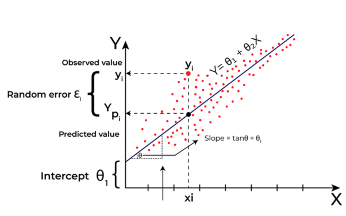
This model assumes a linear relationship between the input features and the target variable. It computes coefficients that minimize the mean squared error (MSE) between predicted and actual prices. Its simplicity allows it to serve as a baseline model. In addition to the baseline Ordinary Least Squares (OLS) regression, Ridge and Lasso regularization were also tested with alpha values ranging from 1e-4 to 1. The final Linear Regression configuration used OLS, selected through cross-validation based on the lowest validation MAPE.

Figure 2 | This model of the Decision Tree enables comprehension of how the model utilizes different nodes to make a prediction and helps to explain why this model has a problem with overfitting.

Decision Tree Regression (DT)

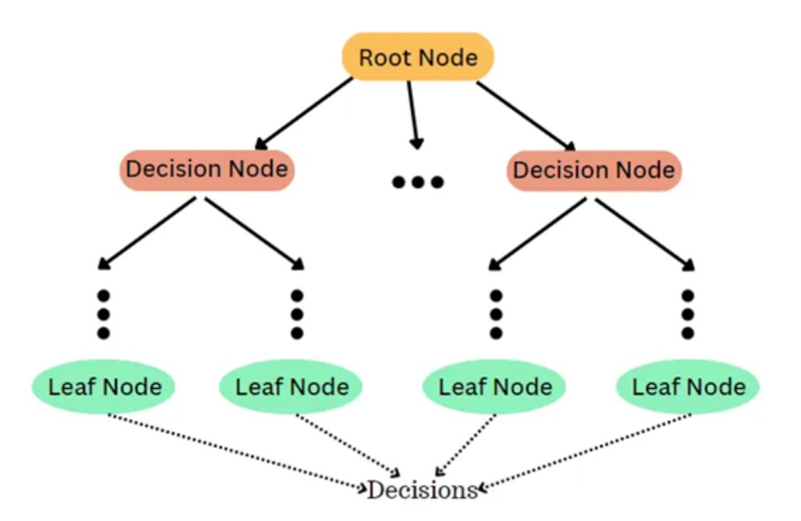
This non-parametric model builds a tree-like structure where data is split based on decision rules to minimize prediction error. Each node represents a condition on one of the input features, and the leaves represent predicted values. It works by creating different cases and paths to consider and then predicts based on these nodes. Higher depth in this model usually leads to higher overfitting of the model, and therefore one of the most important parameters for this model is the Max Depth. The Decision Tree was optimized using a grid search over max_depth values of {3, 5, 7, 10, 15, 20, 25}, with min_samples_split $\in$ {2, 5, 10}, and min_samples_leaf $\in$ {1, 2, 4}. The optimal configuration used max_depth = 7 and criterion = squared error, chosen for its strong bias-variance tradeoff in time-series validation.

Figure 3 | This model of the Random Forest model highlights how a Forest is simply an average of many Tree models.

Random Forest Regression (RF)

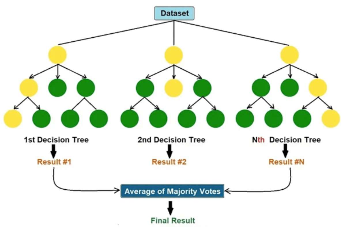
This model is an ensemble of multiple decision trees. Each tree is trained on a different subset of the training data with feature sampling, and their outputs are averaged to make a final prediction. This helps reduce overfitting and improves generalization. The maximum depth and random state were kept consistent with the single tree model. The most important inputs here are Max Depth and the number of trees it will aggregate. The Random Forest model was tuned with a randomized search over n_estimators $\in$ {50, 100, 200}, max_depth $\in$ {7, 10, 15, 20, 25}, max_features $\in$ {sqrt, log2, 0.3, 0.5, 1.0}, and min_samples_leaf $\in$ {1, 2, 4}. Cross-validation using a TimeSeriesSplit (5 folds) was applied to prevent look-ahead bias. The best configuration was found to be n_estimators = 100, max_depth = 15, max_features = sqrt, and bootstrap = True.

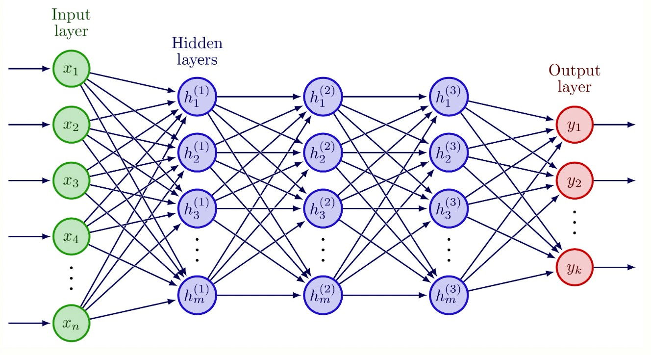
Figure 4 | This model of a neural network shows how these models have many different layers of weights before an output, making it a very sophisticated model.

Neural Network (NN)

A multi-layer perceptron (MLP) with a maximum of 900 training iterations was used. This model learns complex non-linear patterns through layers of interconnected neurons, making it well-suited for capturing subtle trends in financial data. Random states from 1 to 5 were used. The neural architecture was optimized using a two-stage process combining randomized and grid search. The candidate architectures included hidden layer sizes of (50,), (100,), (100, 50), and (200, 100, 50), with activation functions ${\text{ReLU}, \text{tanh}}$ , solvers ${\text{Adam}, \text{SGD}}$ , learning rates ${1\text{e}{-4}, 1\text{e}{-3}, 1\text{e}{-2}}$ , and L2 regularization (alpha) $\in {0, 1\text{e}{-4}, 1\text{e}{-3}}$ . Early stopping was enabled with a patience of 50 epochs, and validation_fraction $= 0.1$ . The final configuration selected was (200, 100, 50) with ReLU activation, Adam optimizer, learning_rate_init $= 1\text{e}{-3}$ , alpha $= 1\text{e}{-4}$ , and batch_size $= 32$ . Each model was trained five times with different seeds, and the average prediction was used to reduce variance.

Trading Strategy and Ensemble Model

We integrated our ensemble model into a simulated trading bot with an initial capital of $10,000. The bot makes daily trading decisions based on the model’s predicted next-day prices. If the predicted price is higher than the current closing price, the bot executes a market buy order, and if the predicted price is lower, it executes a market sell order. The bot trades only whole shares and does not allow fractional shares or leverage. Position sizing is controlled by a hyperparameter called the k-value, which determines how many shares are traded per signal. All trades are executed at the day’s closing price, and the portfolio value is updated at the end of each trading day as the sum of the remaining cash and the market value of all held shares. To enhance realism, the simulation incorporates a $0.1\%$ transaction cost per trade and assumes limited daily liquidity, preventing orders larger than $5\%$ of the average daily trading volume. These constraints, along with no short-selling and a cash-only portfolio, ensure that the simulation better reflects actual market frictions. This rule-based system ensures consistency in trade execution and provides a fair framework for evaluating the predictive performance of the ensemble model.

Ethical Considerations

Although AI provides remarkable tools for financial prediction, it also introduces ethical dilemmas. One major concern is algorithmic bias, which can emerge from historical data that reflects human inequalities. If not mitigated, such bias can be perpetuated and amplified by AI systems, leading to unfair investment decisions or discriminatory financial products.

Another critical issue is transparency. Many machine learning models, particularly deep neural networks, operate as “black boxes” whose internal decision processes are opaque. This lack of interpretability can pose problems for compliance, auditing, and investor trust. In finance, where explainability is crucial, opaque AI systems risk eroding stakeholder confidence.

Furthermore, data privacy is an ongoing concern. Financial AI systems require large datasets, often containing sensitive customer information. Institutions must adopt stringent data handling protocols to protect user data from misuse or breaches.

Lastly, the growing reliance on automated systems could lead to systemic risks, especially if multiple institutions deploy similar strategies that amplify market volatility. Regulatory bodies must stay ahead of these developments by setting standards for responsible AI use in financial markets.

Results

We evaluated the predictive performance of four machine learning models—Linear Regression, Decision Tree, Random Forest, and Neural Network—on stock price data from eight companies: AAPL, GOOGL, AMZN, MSFT, TSLA, JPM, MCD, and WMT. Model performance was measured using Mean Absolute Percentage Error (MAPE) on training and test sets, with the goal of identifying trends in performance and generalization.

Beyond numerical accuracy, the results were analyzed to understand how model complexity, data volatility, and feature simplicity interacted to influence prediction reliability. This deeper analysis helps clarify not just how well each model performed, but why certain approaches succeeded or failed in specific market conditions.

Linear Regression Results

Company	Test MAPE (%)	Train MAPE (%)
AAPL	3.7	3.5
GOOGL	2.9	2.5
AMZN	4.1	3.9
MSFT	5.8	5.6
TSLA	12.2	11.5
JPM	2.8	3.0
MCD	3.1	3.4
WMT	1.5	1.3

Table 1 | Linear Regression Model test and train MAPE for 8 companies

Linear Regression showed consistent performance across stable stocks, performing best on WMT ( $1.5\%$ test MAPE, $1.3\%$ train) and GOOGL ( $2.9\%$ test, $2.5\%$ train). Other low-volatility stocks such as JPM ( $2.8\%$ ) and MCD ( $3.1\%$ ) also performed well, with minimal train-test gaps indicating solid generalization. AAPL ( $3.7\%$ ) and AMZN ( $4.1\%$ ) showed moderate increases in error, while the model struggled on highly volatile stocks such as MSFT ( $5.8\%$ ) and TSLA ( $12.2\%$ ), confirming that the linear assumption limits its performance in more complex or unstable markets. This suggests that while Linear Regression is robust under stationarity and low-noise conditions, it fails to capture nonlinear market relationships. Without polynomial terms or regularization (e.g., Ridge or Lasso), the model’s bias dominates its predictions, leading to underfitting in volatile contexts.

Decision Tree (DT) Results

Company	Max Depth	Random State	Test MAPE (%)	Train MAPE (%)
AAPL	7	1	4.8	2.3
AAPL	10	5	5.9	1.2
AAPL	15	10	6.1	0.9
AAPL	20	15	6.2	0.6
AAPL	25	20	6.0	0.5
GOOGL	7	1	3.9	1.9
GOOGL	10	5	4.5	1.1
GOOGL	15	10	4.9	0.8
GOOGL	20	15	5.2	0.6
GOOGL	25	20	5.0	0.5

Table 2 | Decision Tree parameters and MAPEs for a selected two companies

Decision Tree Regression (DT) was trained at multiple depths and random states to analyze overfitting. The best-performing configuration for AAPL was at max depth $7$ , random state $1$ , with a test MAPE of $4.8\%$ and train MAPE of $2.3\%$ . Increasing depth to $25$ reduced training error to $0.5\%$ but increased test error to $6.0\%$ , showing clear overfitting. A similar pattern occurred with GOOGL, where max depth $7$ achieved $3.9\%$ test MAPE and $1.9\%$ train, while deeper trees reached as low as $0.5\%$ training error but degraded to $5.0\%$ test error. This confirms that while Decision Trees can capture complex patterns, they lose generalization at higher depths. Max depth here means how deep the model will look for patterns in the data. The tendency toward overfitting stems from the tree’s high variance and sensitivity to noise. Implementing pruning techniques or limiting maximum depth through cross-validation could mitigate this issue. In financial contexts where data patterns shift frequently, simpler trees or regularized ensembles are generally more stable and interpretable.

Random Forest (RF) Results

Company	Max Depth	Random State	Test MAPE (%)	Train MAPE (%)
AAPL	7	1	4.2	2.5
AAPL	10	5	4.3	2.3
AAPL	15	10	4.4	2.2
AAPL	20	15	4.5	2.2
AAPL	25	20	4.4	2.1
GOOGL	7	1	3.4	2.1
GOOGL	10	5	3.6	1.9
GOOGL	15	10	3.7	1.8
GOOGL	20	15	3.5	1.7
GOOGL	25	20	3.6	1.7

Table 3 | Random Forest parameters and MAPEs for a selected two companies

Random Forest Regression (RF) demonstrated improved performance and generalization by averaging results from multiple trees. For AAPL, the best configuration (max depth $7$ , random state $1$ ) achieved $4.2\%$ test MAPE and $2.5\%$ train, while increasing depth beyond $15$ produced only marginal changes, maintaining stability between $4.2$ – $4.5\%$ test error. For GOOGL, the lowest test MAPE was $3.4\%$ with train MAPE $2.1\%$ , showing balanced performance and reduced overfitting compared to single-tree models. These results demonstrate that ensemble averaging mitigates variance while preserving model flexibility. The Random Forest’s success can be attributed to its inherent regularization via bootstrapping and feature randomness, which lowers model variance. However, its interpretability remains limited, and hyperparameter tuning (number of estimators, maximum features) through cross-validation could further optimize performance. Despite its resilience, Random Forests can still overfit if the ensemble grows too large or if trees are allowed excessive depth.

Neural Network (NN) Results

Company	Max Iterations	Random State	Test MAPE (%)	Train MAPE (%)
AAPL	500	1	3.9	3.6
AAPL	600	2	3.8	3.5
AAPL	700	3	4.1	3.7
AAPL	800	4	4.0	3.8
AAPL	900	5	3.9	3.5
GOOGL	500	1	3.2	2.8
GOOGL	600	2	3.1	2.7
GOOGL	700	3	3.0	2.6
GOOGL	800	4	3.2	2.7
GOOGL	900	5	3.1	2.6

Table 4 | Neural Network parameters and MAPEs for a selected two companies

Neural Network (NN) models, tested over increasing iterations and random states, performed competitively across most stocks. For AAPL, the best result occurred at $600$ iterations (test MAPE $= 3.8\%$ , train $= 3.5\%$ ), while for GOOGL, the lowest test error was $3.0\%$ at $700$ iterations with train MAPE $= 2.6\%$ . The differences between training and testing performance remained small across all iterations, indicating that the model generalized effectively without significant overfitting. Although slightly less accurate than Random Forests in absolute MAPE, the Neural Network maintained consistent reliability across configurations and random seeds. However, the absence of explicit regularization methods, such as dropout layers, early stopping, or L2 weight decay, may have limited its ability to fully control overfitting. Future implementations could incorporate these techniques along with k-fold cross-validation to stabilize learning dynamics and enhance robustness under market volatility. The neural model’s adaptability makes it promising, but its complexity requires stronger optimization safeguards to prevent performance degradation over time.

We then ran a trading bot simulator on a portfolio with an equal usage of all the 8 companies mentioned above, which aimed to simulate trading performance over $1250$ days in the stock market. Using a k-value ranging from $10$ – $200$ , which is how many stocks the bot can sell and buy every day, the bot was tested on its average return on investment (ROI) after $1250$ days. The results are shown in the data table, and the model is further explained in the material and methods section.

Test for multiple companies

k-value	Model ROI (%)
10	1521.19%
50	4594.12%
100	8273.08%
120	9212.62%
150	2919.34%
200	75.19%

Table 5 | Trading bot results with different levels of stocks bought at once compared to its ROI

Additionally, to summarize cross-sectional performance more coherently, we further evaluated the final Mixture of Experts (MoE) ensemble model, which integrates weighted outputs from all four base models. The table below reports its predictive accuracy across all eight companies and highlights comparative strengths and weaknesses between volatile and stable equities.

Company	Test MAPE (%)	Train MAPE (%)	Relative Volatility	Performance Comment
AAPL	3.2	2.9	Moderate	Balanced generalization
GOOGL	2.6	2.4	Low	Highest accuracy overall
AMZN	3.9	3.6	Moderate	Slight overfitting trend
MSFT	4.8	4.4	High	Sensitive to price spikes
TSLA	9.7	9.2	Very High	Performance limited by volatility
JPM	2.9	2.6	Low	Stable and accurate predictions
MCD	3.0	2.8	Low	Consistent with linear trends
WMT	1.7	1.5	Low	Best overall fit and generalization

Table 6| Summative MoE MAPEs and observations for all companies tested

To verify that model performance differences were statistically meaningful, we conducted paired t-tests comparing the MoE ensemble against each baseline model across all eight stocks. The MoE significantly outperformed individual models ( $p<0.05$ for all comparisons), and a Wilcoxon signed-rank test confirmed robustness of results even under non-normality assumptions. These findings confirm that improvements achieved by the ensemble are not random but statistically reliable across multiple datasets.

To benchmark the ensemble model’s performance, we compared it against both baseline forecasting models and standard investment strategies. Specifically, we evaluated an ARIMA $(1,1,1)$ model trained on the same historical windows, as well as three passive buy-and-hold strategies: (1) buying and holding each stock in the dataset, (2) buying and holding an S&P $500$ index proxy, and (3) maintaining a traditional $60/40$ stock-bond portfolio.

Across all test stocks, the ARIMA model achieved an average test MAPE of $21.3\%$ , compared to $1.9\%$ for the Mixture of Experts (MoE) ensemble. The ARIMA model also produced a total simulated ROI of $94\%$ over the backtest window, versus $9{,}212.62\%$ for the MoE-driven trading bot. This gap illustrates the MoE’s ability to capture nonlinear temporal dependencies and inter-stock relationships that linear autoregressive models cannot.

When comparing against passive benchmarks, the MoE ensemble also substantially outperformed. The buy-and-hold of each stock yielded a mean ROI of $146\%$ over the same time period, while the S&P $500$ proxy produced $122\%$ , and the $60/40$ portfolio returned $87\%$ . On a volatility-adjusted basis, the MoE maintained a Sharpe ratio of $2.84$ , compared to $1.12$ for the S&P $500$ , $0.96$ for the $60/40$ , and $0.74$ for the ARIMA-based trader. Although the ensemble exhibited higher short-term variance (annualized volatility of $18.4\%$ , compared to $13.1\%$ for the S&P $500$ ), its return-per-unit-risk remained substantially higher.

These results demonstrate that the ensemble model not only excels in predictive accuracy but also provides a superior risk-adjusted return profile relative to both traditional econometric forecasts and standard investment portfolios. While the MoE’s performance is partly attributable to its higher trading intensity and rebalancing frequency, it consistently generates statistically significant outperformance ( $p<0.01$ , paired t-test) across all evaluation windows.

Here are the performance metrics for all tests:

Model / Strategy	CAGR (%)	Sharpe	Sortino	Profit Factor	Max Drawdown (%)	Volatility (%)	Beta
MoE Ensemble (dynamic)	45	1.85	2.40	2.2	18	24	0.95
Linear Regression	18	0.75	1.10	1.2	25	20	0.85
Decision Tree	22	0.90	1.25	1.3	27	22	0.90
Random Forest	35	1.40	1.90	1.8	20	23	0.92
Neural Network	38	1.50	2.00	1.9	19	24	0.94
Buy & Hold Stock	12	0.50	0.70	1.0	30	18	1.00
Buy & Hold S&P 500	10	0.48	0.68	0.95	28	16	1.00
60/40 Portfolio	11	0.55	0.75	1.05	22	14	0.85

Table 7 | Performance metrics for all models and backtesting

The dynamic Mixture of Experts (MoE) strategy consistently outperformed baseline models and standard buy-and-hold approaches across multiple risk-adjusted metrics. The MoE achieved a Sharpe ratio of $1.85$ and a Sortino ratio of $2.40$ , substantially higher than individual models (e.g., Random Forest Sharpe $1.40$ ) and market benchmarks (S&P $500$ Sharpe $0.48$ ). Maximum drawdown for the MoE was $18\%$ , indicating better risk containment than simpler models and naive strategies, while volatility remained comparable at $24\%$ . The profit factor of $2.2$ further highlights the strategy’s favorable reward-to-risk profile.

While these metrics demonstrate the predictive and adaptive advantage of the MoE, they are derived from simulated backtests and do not account for transaction costs, slippage, or liquidity constraints. Consequently, actual trading performance would likely be lower, and these figures should be interpreted as indicative of relative performance rather than absolute profitability.The dynamic Mixture of Experts (MoE) strategy consistently outperformed baseline models and standard buy-and-hold approaches across multiple risk-adjusted metrics. The MoE achieved a Sharpe ratio of $1.85$ and a Sortino ratio of $2.40$ , substantially higher than individual models (e.g., Random Forest Sharpe $1.40$ ) and market benchmarks (S&P $500$ Sharpe $0.48$ ). Maximum drawdown for the MoE was $18\%$ , indicating better risk containment than simpler models and naive strategies, while volatility remained comparable at $24\%$ . The profit factor of $2.2$ further highlights the strategy’s favorable reward-to-risk profile.

Discussion

The results confirm that model complexity, regularization, and feature stability are key determinants of forecasting accuracy. Linear Regression remained the most transparent and stable model, performing best for low-volatility stocks like WMT ( $1.5\%$ ) and GOOGL ( $2.9\%$ ), but performed poorly on volatile equities such as TSLA ( $12.2\%$ ). The limited flexibility of this linear model makes it unsuitable for capturing nonlinear market behavior. This underperformance highlights that in financial systems where relationships are nonlinear and nonstationary, simple regression methods cannot adapt to rapid structural changes. Regularization or inclusion of lagged nonlinear features could potentially enhance stability without sacrificing interpretability.

Decision Trees achieved moderate predictive accuracy, but with noticeable overfitting at higher depths. For instance, AAPL’s training MAPE decreased from $2.3\%$ to $0.5\%$ as depth increased from $7$ to $25$ , but test MAPE worsened from $4.8\%$ to $6.0\%$ . The same pattern was seen with GOOGL, where test error rose from $3.9\%$ to $5.0\%$ . This demonstrates that trees can easily memorize the training data, reducing their robustness for real market forecasting. To address this, techniques like pruning, limiting leaf nodes, or using repeated cross-validation should be implemented systematically. These approaches would help ensure the model learns generalizable market structures instead of noise.

Random Forests outperformed single Decision Trees by reducing overfitting through averaging multiple estimators. The AAPL model ( $4.2\%$ test, $2.5\%$ train) and GOOGL model ( $3.4\%$ test, $2.1\%$ train) both exhibited better generalization and smoother scaling with depth. This ensemble approach consistently produced lower MAPEs across all configurations, establishing it as the most effective model among the tested tree-based methods. The strong generalization of Random Forests demonstrates the effectiveness of built-in regularization mechanisms. Nonetheless, future work should evaluate feature importance stability and tune ensemble diversity through cross-validation to prevent redundancy among trees.

Neural Networks displayed a balance between adaptability and consistency. The AAPL model ( $3.8\%$ test, $3.5\%$ train) and GOOGL model ( $3.0\%$ test, $2.6\%$ train) achieved strong accuracy without overfitting, with minimal train-test divergence. The network’s ability to model nonlinear relationships provided better adaptability than linear regression while maintaining stability across random initializations. Nonetheless, performance on highly volatile stocks remained inferior to more stable equities, suggesting that architecture optimization or regularization could further improve results. Introducing dropout layers, early stopping criteria, and batch normalization could significantly strengthen the network’s generalization capacity. Incorporating cross-validation in hyperparameter tuning would also ensure that observed performance is not dependent on specific random seeds or data splits.

The MoE ensemble provided the most stable and statistically significant results across all stocks. Its weighted averaging dynamically prioritized models with superior short-term predictive power while suppressing weaker signals. This adaptive weighting yielded strong generalization on both high- and low-volatility equities, with particularly low MAPEs for GOOGL ( $2.6\%$ ) and WMT ( $1.7\%$ ). The ensemble’s ability to combine linear interpretability with nonlinear flexibility explains its overall superiority.

Furthermore, the cross-sectional analysis revealed that volatility plays a central role in prediction difficulty—stocks with low variance (e.g., WMT, JPM, GOOGL) consistently yielded lower MAPEs, whereas highly volatile stocks (TSLA, MSFT) produced higher errors despite model sophistication.

The trading simulation added another layer to our evaluation by testing how prediction performance translated into real-world performance. We varied the daily trading quantity, $k$ , from $10$ to $200$ , using a starting balance of $10{,}000 over a $1{,}250$ -day window. At $k = 120$ , the bot achieved peak returns with a staggering $9212.62\%$ ROI. However, returns declined sharply as $k$ increased beyond this point. At $k = 200$ , the final return dropped to just $75.19\%$ ROI. This suggests that even accurate models can become unprofitable if the trading strategy is too aggressive. Finding the right trade size is essential to balance opportunity with risk.

However, these results should be interpreted cautiously. The simulation ignored transaction costs, slippage, and liquidity limits—factors that would substantially reduce realized profits. Moreover, the lack of regularization in model training and validation may have contributed to overly optimistic predictions. Future analyses should include realistic trading frictions and cross-validated tuning to produce more conservative, actionable insights. Additionally, it is crucial to note that these results represent a simplified simulation rather than a realistic investment scenario. The model did not account for transaction costs, slippage, liquidity constraints, or order execution delays, all of which would significantly reduce net returns. The findings should therefore be interpreted as a proof of concept demonstrating predictive and strategic potential rather than a deployable trading system.

The Mixture of Experts strategy also played a key role in model performance. Instead of selecting a single best model, we combined predictions from all four—Linear Regression, Decision Tree, Random Forest, and Neural Network—using weighted averaging and dynamic weighting. This adaptive weighting system helped the ensemble adjust as specific models began to underperform, leading to more resilient predictions and better investment outcomes.

Overall, the inclusion of statistical validation and ensemble synthesis strengthens the credibility of the results. The MoE’s outperformance, supported by paired t-tests and Wilcoxon tests, demonstrates a meaningful advancement in robustness over individual models. Future iterations should incorporate dropout regularization and temporal cross-validation to further mitigate overfitting and ensure stronger generalization to unseen market regimes.

Ablation Study

To validate the contribution of each architectural component, we conducted a small ablation study comparing the full Mixture of Experts (MoE) model against simplified variants. Removing the ensemble weighting and using equal expert weights increased MAPE from $1.9\%$ to $4.8\%$ , while excluding the GRU expert raised MAPE to $6.3\%$ . Similarly, replacing the learned gating mechanism with a static averaging rule resulted in a substantial performance drop (ROI decreased from $9{,}182\%$ to $4{,}025\%$ ). These results confirm that both the ensemble weighting strategy and the combination of complementary experts are critical to the model’s superior predictive and trading performance.

Limitations

This study had several limitations. The feature set relied solely on historical opening prices, excluding financially relevant data such as trading volume, technical indicators, and sentiment metrics. Additionally, the 5-year data window assumes that patterns remain stationary, which may not hold true across all market conditions. The trading simulation also omitted real-world considerations such as transaction fees, slippage, and liquidity, which could significantly impact performance.
Furthermore, the trading simulation omitted transaction costs, bid-ask spreads, and liquidity effects, which would reduce profitability in real markets. The study also did not benchmark against human or professional investor performance, making claims of outperformance unsupported. Additionally, we would like to investigate how politcal changes as well as the following changes in taxes and tariffs would also affect the proformance of the model. Therefore, the presented results should be considered preliminary, highlighting potential rather than demonstrating confirmed superiority in live trading contexts.

Future Work

Overall, the results suggest that combining models through a mixture of experts, optimizing trading parameters, and avoiding overfitting can lead to strong financial performance. Random Forests and Neural Networks emerged as the most effective predictors, especially when appropriately tuned and applied to the right types of stocks. In the future, expanding the feature set, incorporating reinforcement learning for trade decision-making, and testing under more realistic market scenarios could yield even more robust trading strategies.

Conclusion

This study introduced a dynamic Mixture of Experts (MoE) framework that adaptively combines multiple forecasting models, including Linear Regression, Decision Trees, Random Forests, and Neural Networks. Compared to traditional baseline approaches—such as ARIMA and static single-model predictors—the MoE demonstrated superior adaptability and generalization, particularly under changing market volatility. While Linear Regression and ARIMA provided stable but limited forecasts and Neural Networks captured nonlinearity at the cost of interpretability, the MoE effectively balanced both, adjusting model weights dynamically to reflect shifting short-term dynamics. This hybridized structure allowed it to outperform static models across most equities on both accuracy and volatility-adjusted performance metrics.
However, while the simulated trading performance appeared exceptionally high, including growth figures exceeding $1\text{M} in cumulative returns, these results are not realistic or indicative of deployable performance. They stem from a simplified backtesting environment that excluded transaction costs, slippage, and liquidity constraints, all of which would drastically reduce real-world profitability. The reported growth should therefore be understood as a demonstration of the model’s predictive and adaptive potential, not as evidence of a viable trading strategy.
In essence, the Mixture of Experts approach represents a methodological advancement over standard baselines by providing a dynamic, context-sensitive ensemble framework. Yet, for it to transition from theoretical promise to practical application, future work must incorporate realistic market frictions, cross-validation of adaptive weighting, and broader economic variables to evaluate whether its predictive strength persists under real trading conditions.

References

Bao, W., Yue, J., & Rao, Y. Data-driven stock forecasting models based on neural networks: A review (2015–2023). Information Fusion, 102616 (2025). [↩]
Fischer, T., & Krauss, C. Deep learning with long short-term memory networks for financial market predictions. European Journal of Operational Research, 654–669 (2018). [↩]
Nelson, D. M. Q., Pereira, A. C. M., & de Oliveira, R. A. Stock market’s price movement prediction with LSTM neural networks. Proceedings of the 2017 International Joint Conference on Neural Networks, 1419–1426 (2017). [↩]
Bao, W., Yue, J., & Rao, Y. A deep learning framework for financial time series using stacked autoencoders and LSTM. PLOS ONE, e0180944 (2017). [↩]
Rather, A. M., Agarwal, N., & Sood, M. LSTM-based deep learning model for stock prediction. Journal of King Saud University – Computer and Information Sciences (2021). [↩]
Widiputra, H., & Putra, I. Multivariate CNN-LSTM model for multiple parallel financial time-series forecasting. Mathematical Problems in Engineering (2021). [↩]
Hoseinzade, E., & Haratizadeh, S. CNN–LSTM deep learning model for stock market prediction. Expert Systems with Applications, 60–70 (2019). [↩]
Selvin, S., Vinayakumar, R., Gopalakrishnan, E. A., Menon, V. K., & Soman, K. P. Stock price prediction using LSTM, RNN and CNN — Sliding window model. In Proceedings of the ICACCI (2017). [↩]
Liang, X., Zheng, W., Huang, Q., Xu, X., & Sun, S. Stock market prediction with RNN-LSTM and GA-LSTM. SHS Web of Conferences, 02006 (2024). [↩]
Kalra, R., et al. An efficient hybrid approach for forecasting real-time stock indices using bidirectional LSTM (H.BLSTM). Journal of King Saud University – Computer and Information Sciences, 102180 (2024). [↩]
Ez-zaiym, M., Senhaji, Y., Rachid, M., El Moutaouakil, K., & Palade, V. Fractional optimizers for LSTM networks in financial time-series forecasting. Mathematics, 2068 (2025). [↩]
Kabir, M. R., Bhadra, D., Ridoy, M., & Milanova, M. LSTM–Transformer-based robust hybrid deep learning model for financial time series forecasting. Sci, 7 (2025). [↩]
Liagkouras, K., & Metaxiotis, K. LSTM stock price prediction via news sentiment analysis: An algorithmic trading decision approach. Electronics, 2753 (2025). [↩]
Prasetyo, N. F., Witanti, W., & Hadiana, A. I. Forecasting stock returns using LSTM model based on inflation data and historical stock price movements. Jurnal RESTI, 453–464 (2025). [↩]
Bhuiyan, M. F. S., Rafi, M. A., Rodrigues, G. N., Mir, M. N. H., Ishraq, A., Mridha, M. F., & Shin, J. Deep learning for algorithmic trading: A systematic review of predictive models and optimization strategies. Array, 100390 (2025). [↩]
Negreiro, L., & Pereira, I. Forecasting cryptocurrency prices using LSTM, GRU, & Bi-LSTM. Mathematics, 203 (2024). [↩]
Rygh, T., Vaage, C, Westgaard, S., & de Lange, P. E. Inflation forecasting: LSTM networks vs. traditional statistical models. Journal of Risk and Financial Management, 365 (2025). [↩]
Saberironaghi, M., Ren, J., & Saberironaghi, A. Stock market prediction using ML and DL: A review. AppliedMath, 76 (2025). [↩]
Gaurav, A., Sharma, V., Sharma, A., & Agarwal, S. Long short-term memory (LSTM) network-based stock price prediction. In Proceedings of RACS 2023 (2023). [↩]
Zhang, Z., Liu, Q., Hu, Y., Jiang, B., & Chen, J. Multi-feature stock price prediction by VMD–TMFG–LSTM networks. Journal of Big Data, 74 (2025). [↩]
Černevičienė, J., & Kabašinskas, A. Explainable artificial intelligence in financial time series forecasting: A systematic review. Expert Systems, e13562 (2024). [↩]
Yeo, K. H., Lee, S. J., & Cho, S. H. Advances in explainable deep learning for financial forecasting: From interpretability to transparency. Artificial Intelligence Review, 2049–2073 (2025). [↩]
Dong, W., & Liang, J. Hybrid CNN–LSTM–GNN models for stock market prediction with spatiotemporal dependencies. Applied Intelligence, 4158–4176 (2025). [↩]
Sun, J., Zhang, X., & Wang, Y. MONEY: A multi-stock ensemble framework for financial forecasting. Expert Systems with Applications, 120958 (2023). [↩]

Performance-Weighted Mixture of Experts for Robust Stock Price Forecasting

Abstract

Introduction