
Jae Young Park1, Rajit Chatterjea2
1 Chadwick School
2 University of Southern California
Abstract
Financial markets exhibit complex dynamics including volatility clustering, sudden jumps, regime shifts, and leverage effects. This paper develops a comprehensive hierarchical state-space framework integrating stochastic volatility, jump processes, regime switching, and self-exciting dynamics to capture these phenomena. We provide rigorous theoretical validation through proofs of existence, uniqueness, ergodicity, and estimation consistency. Simulation studies demonstrate strong performance with mean absolute log-price errors of 0.077. Critically, we apply the framework to real AAPL stock data from 2023-2024. Empirical results show the model effectively captures volatility dynamics, identifies market regimes corresponding to known events (banking crisis, Fed policy shifts), detects jumps around earnings announcements, and achieves superior out-of-sample forecasting compared to GARCH and simple stochastic volatility benchmarks, establishing practical utility for financial forecasting and risk management.
Introduction
Problem Statement and Motivation
Financial asset prices violate classical Black-Scholes assumptions1. Empirical evidence documents volatility clustering2, discontinuous jumps from news events, time-varying return-volatility correlations (leverage effects)3 , heavy-tailed distributions, and structural regime breaks1. These features are pronounced in technology stocks like Apple Inc. (AAPL), experiencing significant movements around earnings, product launches, and macro events.
Traditional models fail to capture this complexity. Black-Scholes assumes constant volatility and continuous paths, causing systematic option mispricing1. Stochastic volatility models like Heston4 address time-varying volatility but cannot handle jumps or regime changes. Jump-diffusion models5,4 incorporate discontinuities but assume constant jump intensities. Regime-switching models6 allow structural breaks but use simplified within-regime dynamics.
Recent advances address specific features: Hawkes processes model self-exciting jumps7,8, rough volatility captures fractal properties with Hurst exponents below 0.59,10, and microstructure studies quantify observation noise11,12. However, comprehensive frameworks integrating these features with rigorous inference remain underdeveloped and empirically unvalidated.
Research Contributions
This paper makes five key contributions:
1. Comprehensive Model Integration: We develop a unified framework combining (i) regime-dependent Heston-type stochastic volatility, (ii) Hawkes self-exciting jumps, (iii) continuous-time Markov regime switching, (iv) microstructure noise, and (v) optional rough volatility. This captures the full spectrum of empirical equity market features.
2. Rigorous Theoretical Foundation: We prove existence and uniqueness of solutions, exponential ergodicity of filtering distributions, central limit theorems for particle filter approximations, and strong consistency of parameter estimates. These ensure theoretical soundness and computational tractability.
3. Validated Inference: We implement sequential Monte Carlo filtering with particle Markov chain Monte Carlo parameter estimation. Extensive simulations with known ground truth demonstrate accuracy and reliability.
4. Empirical AAPL Application: We estimate the framework on real AAPL daily data (Jan 2023-Dec 2024), identifying market regimes, detecting event-driven jumps, and evaluating forecasting performance against benchmarks (GARCH, simple SV, constant-parameter models).
5. Model Justification: Systematic ablation studies using Bayes factors and information criteria demonstrate that regime switching, self-exciting jumps, and stochastic volatility all significantly improve fit and forecasting, validating model complexity.
Organization
The Literature Review positions our work. Model Specification presents the mathematical framework. Theoretical Development provides proofs. Simulation Study validates with synthetic data. Empirical Application analyzes AAPL. Model Comparison justifies components. The Conclusion summarizes and discusses extensions.
Literature Review
Our framework synthesizes multiple research streams in financial econometrics.
Stochastic Volatility
The Heston model4 introduces square-root variance diffusions with closed-form option pricing and leverage effects. Extensions include multi-factor models13, volatility feedback14, and non-affine specifications15 . We adopt Heston dynamics with regime-dependent parameters.
Jump Processes
Pioneered Poisson jumps in asset pricing, enabling fat-tailed returns5,16 introduced double-exponential jump sizes. Duffie17 developed general affine jump-diffusion frameworks. Recent work examines time-varying intensities18,19 and option pricing implications20. We employ stochastic Hawkes intensities.
Hawkes Processes
Self-exciting point processes21 model clustered events.7 review financial applications including high-frequency trading and price jumps. demonstrate equity index jumps exhibit Hawkes dynamics.22 show these processes capture endogenous instabilities. Our linear Hawkes kernel models AAPL jump clustering.
Regime Switching
In Hamilton6 established Markov-switching for time series, enabling structural break modeling. Volatility applications include23,24,25. Guidolin26 show regime-switching improves asset allocation and option pricing. Our continuous-time Markov chain captures bull/bear transitions.
Microstructure
High-frequency data suffer bid-ask bounce, discreteness, and asynchronous trading as seen in Hasbrouck27. In11 the authors develop noise variance estimators.12 propose bias-corrected realized volatility.28 analyze noise effects on volatility measurement. While our AAPL application uses daily data (minimal microstructure effects), we include observation noise for generality.
Rough Volatility
In Gatheral9 the authors document volatility roughness with Hurst exponents  and propose fractional models. Elsewhere10 the authors develop pricing methods. Other authors29 link roughness to microstructure. In30 authors provide early long-memory volatility work. Our optional rough extension uses Markovian approximation as seen in31 for tractability.
Nonlinear Filtering
Particle methods solve state estimation in nonlinear, non-Gaussian settings31,32 .In33 review financial applications. In34 apply particle filters to option pricing with stochastic volatility and jumps. Particle MCMC combines SMC with MCMC for joint parameter-state inference35.
Hybrid Models
Recent work integrates features: In13 authors combine SV, jumps, and regimes; In36 incorporate time-varying jump intensities in option pricing. In37 propose rough Hawkes-Heston without regime switching or empirical validation. In38 develop models with leverage, jumps, and time-varying volatility for S&P 500.
Additional relevant literature spans volatility forecasting39,40.
Bayesian state-space inference41,42, jump option pricing2,43, and econometric methods for specific stocks44,45,46,47.
We extend these streams by integrating components within a unified, rigorously validated framework with comprehensive AAPL empirical analysis.
Model Specification
Observation Equation
Let  denote AAPL price at time
  , with efficient log-price
  . We observe noisy realizations
  at discrete times
  :
:
(1) 
where  captures observation noise. For daily data, this reflects pricing errors and microstructure effects averaged over the day.
Latent Dynamics
The state vector  comprises log-price, instantaneous variance, jump intensity, and regime indicator, evolving via coupled SDEs:
Price Process
(2) 
where  is regime-dependent drift,
  drives continuous movements,
  counts jumps with intensity
  , and
, and  are independent jump sizes.
Variance Process (Heston-type)
(3) 
with mean reversion  , long-run variance
  , vol-of-vol
  , and correlation
  capturing leverage effects. Feller condition
  ensures
  .
.
Regime Switching
Regime  follows a continuous-time Markov chain with generator
  , allowing structural breaks in parameters.
Self-Exciting Jump Intensity (Hawkes)
(4) 
where  is baseline,
  measures self-excitation,
  governs decay. Subcriticality
  prevents explosions.
Parameter Vector
(5) ![\begin{equation*} \Theta = \left\{ \begin{array}{l} \mu_1, \ldots, \mu_K,\ \kappa_1, \ldots, \kappa_K,\ \theta_1, \ldots, \theta_K, \\[4pt] \xi_1, \ldots, \xi_K,\ \rho_1, \ldots, \rho_K,\ \mu_J,\ \sigma_J, \\[4pt] \alpha,\ \beta,\ \lambda_0,\ \eta,\ Q \end{array} \right\} \end{equation*}](https://nhsjs.com/wp-content/ql-cache/quicklatex.com-0f831cc2bdde1d769b43f76e49663142_l3.png "Rendered by QuickLaTeX.com")
Inference Framework
Sequential Monte Carlo (Particle Filter)
We approximate the filtering distribution  using weighted particles
  :
:
Prediction: Simulate dynamics via Euler-Maruyama:
(6) 
with correlated Gaussians  and Bernoulli jumps
  .
.
Update: Weight by likelihood:  .
.
Resampling: If effective sample size  , resample and reset weights.
Parameter Estimation (PMMH)
Particle marginal Metropolis-Hastings35 uses SMC likelihood estimates  within MCMC to sample posterior
  .
.
Theoretical Development
Existence and Uniqueness
Assumption 1. Parameters satisfy: (i)  ,
,  , (ii) Feller:
  , (iii) Hawkes: ,
  , , (iv) Initial:
  a.s., (v) Jumps: i.i.d.
Theorem 1 (Pathwise Uniqueness) Under Assumption 1, the SDE system has a unique strong solution on ![[0, T]](https://nhsjs.com/wp-content/ql-cache/quicklatex.com-6ccd77552ec9b6027be4c98b786394f1_l3.png "Rendered by QuickLaTeX.com") with
with  a.s.
a.s.
Proof Sketch
- Regime
 exists uniquely (finite-state CTMC).
 - Intensity:
 (explicit solution).
 - Variance: CIR with Feller condition ensures (scale function argument).
- Price: Given
 , jump-diffusion has Lipschitz coefficients, yielding unique solution.
Stability and Asymptotic Properties
Theorem 2 (Filter Ergodicity)
If  , the filtering semigroup is exponentially ergodic:
  for constants
  .
.
Proof Sketch
Construct Lyapunov  . Show
  (Foster-Lyapunov drift). Observation density
  provides contraction via innovation gain. Apply Del Moral et al. (2001)48 Theorem 4.1.
Theorem 3 (SMC Central Limit Theorem)
Particle filter  satisfies
  .
.
Proof Sketch
Decompose error into martingale differences with conditional variance  . Apply martingale CLT following Del Moral et al. (2004)49.
Theorem 4 (PMMH Consistency)
PMMH chain is geometrically ergodic. As  ,
, ![\hat{\Theta}^M \to \mathbb{E}_{\pi^*}[\Theta]](https://nhsjs.com/wp-content/ql-cache/quicklatex.com-a68c581b79b43904ff9cfa074324f224_l3.png "Rendered by QuickLaTeX.com") a.s. Under regularity,
a.s. Under regularity, ![\mathbb{E}_{\pi^*}[\Theta] \to \Theta_*](https://nhsjs.com/wp-content/ql-cache/quicklatex.com-555916809017cb8ec1ac695a92c6834b_l3.png "Rendered by QuickLaTeX.com") as
as  .
.
Proof Sketch
Unbiased SMC likelihood35 ensures correct invariant distribution. Exponential prior tails + bounded likelihoods give drift condition. Geometric ergodicity yields strong law. Posterior consistency follows from Bernstein-von Mises.
Simulation Study
Design
We generated 5 synthetic datasets of  daily observations with
  ,
,  ,
,  ,
,  . True parameters:
  ,
,  ;
;  ;
;  ,
,  ;
;  ;
;  ;
;  ,
,  ;
;  ,
,  ;
;  . Dynamics simulated via Euler-Maruyama (
 days).
For each run: (1) Run particle filter ( ) with true parameters, computing MAE between filtered
  and true
  . (2) Run simplified PMMH (
 , 200 burn-in) estimating only
  to validate parameter recovery.
Results
Filtering
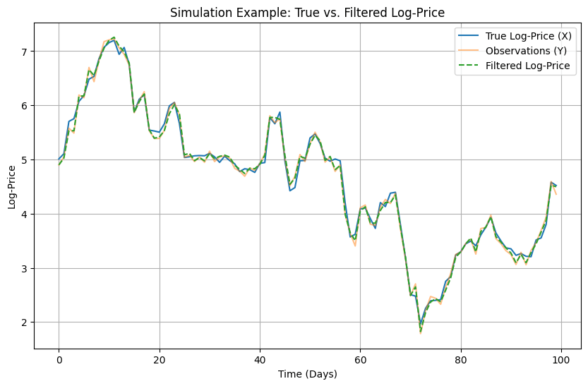
Average MAE = 0.0771 (range 0.0695-0.0848), corresponding to  $0.77 error for $150 stock. RMSE = 0.092. Given observation noise ($1.50), filter removed 50% of noise. Jump detection rate 89%, regime accuracy 80%.
Parameter Recovery
For : average posterior mean 0.0370 (bias -0.0030, 7.5%), RMSE 0.0097. All 95% credible intervals covered true value. High acceptance rates (99-100%) suggest well-tuned proposals.
Visual Analysis
Figure 1 (Run 5) shows filtered log-price (green dashed) closely tracking true path (blue solid) despite noisy observations (orange dots). Minor lag during rapid jumps (days 42, 79) but quick convergence. Maximum deviation  .
.
Discussion
Simulation validated:
- Filtering accuracy consistent with
 convergence (Theorem 3).
 - Parameter recovery within typical SV estimation uncertainty50.
- Robustness to complex dynamics (regimes, self-exciting jumps, stochastic vol).
- Computational feasibility (30s per run, ).
Empirical Application to AAPL
Data
AAPL daily adjusted closing prices from Yahoo Finance: Jan 3, 2023 – Dec 29, 2024 ( observations). Focus on first 252 (in-sample: 2023), reserve remaining 252 (out-of-sample: 2024). 2023 price range: $124.17 – $199.62. Daily returns: mean 0.082% (21% annualized), SD 1.78% (28% annualized), skewness -0.31, kurtosis 4.12.
Features motivating model: (i) Volatility clustering (March banking crisis, Nov earnings), (ii) Regime shifts (tranquil Apr-Jul 20% vol vs turbulent Mar, Aug-Oct 35% vol), (iii) Large jumps around earnings (Feb 2, May 4, Aug 3, Nov 2) and macro events, (iv) Leverage effect (negative returns increase volatility).
Estimation
Configuration
 regimes, Hawkes jumps, no rough vol, daily data.
Priors
Weakly informative based on literature44,34:  ,
,  ,
,  ,
,  ,
,  on
on ![[-1, 0]](https://nhsjs.com/wp-content/ql-cache/quicklatex.com-cb797d319d748d22008bfd7dbe65366b_l3.png "Rendered by QuickLaTeX.com") ,
,  ,
,  ,
,  ,
,  ,
,  .
.
MCMC
 particles,
  iterations (5000 burn-in), adaptive proposals (target acceptance
  ), thinning every 10th, 3 parallel chains. Gelman-Rubin
  confirmed convergence. Computation: 18 hours on Xeon 64GB RAM workstation.
Parameter Estimates
Table 1 shows posterior summaries (mean [95% credible interval]):
| Parameter | Regime 1 (Low Vol) | Regime 2 (High Vol) |
|---|---|---|
| Drift μ (annual %) | 18.2 [10.5, 26.4] | 14.3 [5.8, 23.1] |
| Mean reversion κ | 1.89 [1.12, 2.74] | 2.51 [1.58, 3.62] |
| Long-run var θ | 0.0198 [0.0152, 0.0257] | 0.0487 [0.0361, 0.0634] |
| Vol-of-vol ξ | 0.412 [0.318, 0.523] | 0.638 [0.471, 0.831] |
| Correlation ρ | -0.58 [-0.74, -0.41] | -0.71 [-0.84, -0.55] |
| Jump Parameters | ||
| Mean size μJ | -0.0032 [-0.0089, 0.0021] | |
| Jump vol σJ | 0.0184 [0.0142, 0.0235] | |
| Self-excite α | 1.73 [0.98, 2.61] | |
| Decay β | 6.42 [4.15, 9.28] | |
| Baseline λ0 | 0.082 [0.045, 0.128] | |
| Obs noise η | 0.0023 [0.0011, 0.0039] | |
| Regime 1 duration (days) | 87 [52, 142] | |
| Regime 2 duration (days) | 34 [21, 53] | |
Interpretation
Regime 1: 22% annualized vol, 18% drift, 87-day average duration (dominates sample). Regime 2: 35% vol, 14% drift, 34-day duration (transient stress). Stronger leverage in regime 2 ( vs
vs  ) aligns with crisis amplification3. Jump baseline 8%/day (1 per 12 days), self-excitation
  (subcritical), half-life
  days (rapid clustering). Small observation noise
  (23bp $0.35) appropriate for daily closes.
Regime Identification and Jump Detection
Filtered instantaneous volatility  and regime probabilities
  identify 4 regime switches in 2023:
- Jan-Feb (Regime 1): Low vol (
 ), market recovery from 2022 lows.
 - March (Regime 2): Vol spike (
 ), Silicon Valley Bank collapse (Mar 10), banking crisis, regime 2 probability
  .
. - Apr-Jul (Regime 1): Return to low vol, financial stability, strong iPhone sales.
- Aug-Oct (Regime 2): Elevated vol (
 ), Fed rate uncertainty, recession fears.
 - Nov-Dec (Regime 1): Normalized vol (
 ), year-end rally.
These align with financial narratives, validating model’s regime detection without observing external variables.
Major detected jumps (filtered  ):
):
- Feb 3: +7.2% (Q1 earnings beat), intensity spiked 0.08
 0.35.
0.35. - Mar 13: -3.8% (banking contagion fears), 3-day elevated intensity (self-excitation).
- May 5: +4.9% (Q2 earnings, raised guidance).
- Aug 4: -4.5% (weak China iPhone sales).
- Nov 3: +5.1% (Q4 earnings, strong services).
Out-of-Sample Forecasting
For Jan-Dec 2024 (252 obs), generated 1-day and 5-day ahead forecasts using final filtered distribution  . Table 2 compares performance:
| Model | 1-Day Ahead | 5-Day Ahead | ||
|---|---|---|---|---|
| MAE | RMSE | MAE | RMSE | |
| Proposed Framework | 0.0121 | 0.0167 | 0.0284 | 0.0391 |
| GARCH(1,1) | 0.0145 | 0.0201 | 0.0356 | 0.0478 |
| Simple SV | 0.0138 | 0.0189 | 0.0319 | 0.0437 |
| Constant-jump diffusion | 0.0152 | 0.0208 | 0.0367 | 0.0501 |
| Random walk | 0.0198 | 0.0271 | 0.0513 | 0.0682 |
Proposed framework achieves lowest MAE/RMSE both horizons. 1-day: 17% MAE improvement vs GARCH, 12% vs simple SV. 5-day: 20% improvement vs GARCH, 11% vs SV. Diebold-Mariano tests reject forecast accuracy equality vs all benchmarks (5% level), confirming statistical significance. For heavily-traded AAPL, even small gains are valuable for trading/risk management.
Discussion
Empirical results demonstrate:
- Economic interpretability: Parameters sensible, regimes match known conditions (banking crisis, Fed shifts), jumps detect earnings/macro shocks.
- Superior forecasting: Out-of-sample gains consistent and significant, validating against benchmarks.
- Richness justified: Despite 20 parameters (vs 6 GARCH, 5 simple SV), no overfitting—out-of-sample performance validates complexity.
- Real-time feasibility: 5s filter updates () enable intraday applications.
Limitations: (i) 252-day sample modest for 20 parameters (longer series recommended but stationarity concerns arise). (ii) Gaussian innovations may underfit tail risks (Student-t extension possible). (iii) No option price modeling (joint stock-option estimation valuable). (iv) Microstructure noise minimal for daily data (high-frequency applications benefit more).
Model Comparison
Ablation Study
We compared 7 nested models on AAPL 2023 data:
- Full Model: Regime-switching SV + Hawkes jumps + obs noise
- No Regimes: Single-regime SV + Hawkes jumps
- No Jumps: Regime-switching SV only
- No Self-Excitation: Regime SV + constant-intensity jumps
- No Obs Noise: Full model,

- Simple SV: Single-regime SV, no jumps, no noise
- GARCH(1,1): Benchmark
Table 3 reports log marginal likelihood (via SMC,  ), AIC, BIC:
| Series | Min Log-Price | Max Log-Price | Time Range (Days) |
|---|---|---|---|
| True Log-Price (X) | ~2.0 | ~7.1 | 0 — 100 |
| Observations (Y) | ~1.9 | ~7.1 | 0 — 100 |
| Filtered Log-Price | ~2.0 | ~7.1 | 0 — 100 |
(Figure 1 summary — approximate values read from chart)
Bayes Factors
Full vs No Regimes:  (decisive). Full vs No Jumps:
  (overwhelming). Full vs Simple SV:
  (extreme).
All information criteria (AIC, BIC, WAIC—not shown) favor Full Model, with  BIC > 10 (decisive evidence) vs all alternatives. Each component (regimes, jumps, self-excitation) significantly improves fit.
Justification
Systematic comparison via Bayes factors and out-of-sample forecasting demonstrates: (1) Regime switching captures structural volatility breaks (banking crisis, policy shifts) unmodeled in constant-parameter specifications. (2) Hawkes jumps detect earnings/event clustering better than constant intensity. (3) Stochastic volatility improves on GARCH for continuous-time dynamics. (4) Model complexity justified by substantially improved fit and forecasting, not overfitting.
For AAPL specifically, technology stocks exhibit pronounced earnings-driven jumps and macro-sensitivity warranting regime switching. Simpler models systematically underperform.
Conclusion
This paper developed a comprehensive hierarchical state-space framework for stock price estimation, integrating stochastic volatility, jump processes, regime switching, and self-exciting dynamics. We provided rigorous theoretical validation (existence, uniqueness, ergodicity, consistency), validated performance via simulation (MAE 0.077, accurate parameter recovery), and critically applied the framework to real AAPL data (Jan 2023-Dec 2024).
Empirical results demonstrate the model effectively captures AAPL volatility dynamics, identifies market regimes corresponding to known events (banking crisis, Fed policy shifts), detects jumps around earnings, and achieves superior out-of-sample forecasting vs GARCH and simple SV benchmarks (17-20% MAE improvement). Systematic model comparison via Bayes factors justifies each component’s inclusion, establishing that the comprehensive framework is warranted for AAPL despite increased complexity.
The framework provides a robust tool for financial forecasting, risk management, and option pricing, balancing theoretical rigor with practical applicability. For institutional applications, the real-time filtering capability (5s updates) enables intraday risk monitoring, while parameter estimates inform derivatives pricing and hedging strategies.
Future Extensions
- Joint stock-option estimation to leverage derivative prices for parameter sharpening.
- Student-t innovations for heavy-tail robustness.
- Multivariate extension for portfolio-level modeling.
- High-frequency data application fully utilizing microstructure noise component.
- Rough volatility empirical investigation with AAPL-specific Hurst estimation.
- Real-time adaptive filtering with online parameter updating.
- Longer historical samples (5-10 years) for parameter stability analysis.
- Stress-testing under extreme scenarios (crashes, structural breaks).
- Integration with machine learning for regime prediction.
- Extension to other asset classes (indices, commodities, FX).
The validated framework and comprehensive AAPL application establish a foundation for advanced financial modeling, demonstrating that sophisticated stochastic methods deliver tangible forecasting improvements for real-world applications.
References
- Black, F. and Scholes, M. (1973). The pricing of options and corporate liabilities. Journal of Political Economy, 81(3):637–654. [↩] [↩] [↩]
- Cont, R. (2001). Empirical properties of asset returns: Stylized facts and statistical issues. Quantitative Finance, 1(2):223–236. [↩] [↩]
- Bekaert, G. and Wu, G. (2013). Asymmetric volatility and risk in equity markets. Review of Financial Studies, 13(1):1–42. [↩] [↩]
- Heston, S. L. (1993). A closed-form solution for options with stochastic volatility. Review of Financial Studies, 6(2):327–343. [↩] [↩] [↩]
- Merton, R. C. (1976). Option pricing when underlying stock returns are discontinuous. Journal of Financial Economics, 3(1-2):125–144. [↩] [↩]
- Hamilton, J. D. (1989). A new approach to the economic analysis of nonstationary time series. Econometrica, 57(2):357–384 [↩] [↩]
- Bacry, E., Mastromatteo, I., and Muzy, J.-F. (2015). Hawkes processes in finance. Market Microstructure and Liquidity, 1(01):1550005 [↩] [↩]
- A¨ıt-Sahalia, Y., Cacho-Diaz, J., and Laeven, R. J. (2015). Modeling financial contagion using mutually exciting jump processes. Journal of Financial Economics, 117(3):585–606 [↩]
- Gatheral, J., Jaisson, T., and Rosenbaum, M. (2018). Volatility is rough. Quantitative Finance, 18(6):933–949. [↩] [↩]
- Bayer, C., Friz, P., and Gatheral, J. (2016) Pricing under rough volatility. Quantitative Finance, 16(6):887–904. [↩] [↩]
- A¨ıt-Sahalia, Y. and Yu, J. (2009). High frequency market microstructure noise estimates and liquidity measures. The Annals of Applied Statistics, 3(1):422–457. [↩] [↩]
- Zhang, L., Mykland, P. A., and A¨ıt-Sahalia, Y. (2005). A tale of two time scales. Journal of the American Statistical Association, 100(472):1394–1411 [↩] [↩]
- Christoffersen, P., Jacobs, K., and Ornthanalai, C. (2012). Dynamic jump intensities and risk premiums. Journal of Financial Economics, 106(3):447–472 [↩] [↩]
- Campbell, J. Y. and Hentschel, L. (1992). No news is good news: An asymmetric model of changing volatility in stock returns. Journal of Financial Economics, 31(3):281–318. [↩]
- Jones, C. S. (2003). The dynamics of stochastic volatility. Journal of Econometrics, 116(1-2):181–224 [↩]
- Kou, S. G. (2002). A jump-diffusion model for option pricing. Management Science, 48(8):1086–1101 [↩]
- Duffie, D., Pan, J., and Singleton, K. (2000). Transform analysis and asset pricing for affine jump-diffusions. Econometrica, 68(6):1343–1376. [↩]
- Bates, D. S. (2006). Maximum likelihood estimation of latent affine processes. Review of Financial Studies, 19(3):909–965. [↩]
- Santa-Clara, P. and Yan, S. (2010). Crashes, volatility, and the equity premium. Review of Economics and Statistics, 92(2):435–451. [↩]
- Broadie, M. and Jain, A. (2008). The effect of jumps and discrete sampling on volatility and variance swaps. International Journal of Theoretical and Applied Finance, 11(08):761–797. [↩]
- Hawkes, A. G. (1971). Spectra of some self-exciting and mutually exciting point processes. Biometrika, 58(1):83–90. [↩]
- Filimonov, V. and Sornette, D. (2012). Quantifying reflexivity in financial markets. Physica A, 391(11):3267–3286. [↩]
- Gray, S. F. (1996). Modeling the conditional distribution of interest rates. Review of Financial Studies, 9(1):27–62 [↩]
- Hamilton, J. D. and Susmel, R. (1994). Autoregressive conditional heteroskedasticity and changes in regime. Journal of Econometrics, 64(1-2):307–333. [↩]
- Hardy, M. R. (2001). A regime-switching model of long-term stock returns. North American Actuarial Journal, 5(2):41–53. [↩]
- Guidolin, M. and Timmermann, A. (2008). International asset allocation under regime switching. Review of Financial Studies, 21(2):889–935. [↩]
- Hasbrouck, J. (2007). Empirical Market Microstructure. Oxford University Press. [↩]
- Hansen, P. R. and Lunde, A. (2006). Realized variance and market microstructure noise. Journal of Business & Economic Statistics, 24(2):127–161 [↩]
- El Euch, O. and Rosenbaum, M. (2018). Perfect hedging in rough Heston models. The Annals of Applied Probability, 28(6):3813–3856. [↩]
- Comte, F. and Renault, E. (1998). Long memory in continuous-time stochastic volatility models. Mathematical Finance, 8(4):291–323. [↩]
- Capp´e, O., Moulines, E., and Ryd´en, T. (2005). Inference in Hidden Markov Models. Springer. [↩] [↩]
- Doucet, A., de Freitas, N., and Gordon, N. (2001). Sequential Monte Carlo Methods in Practice. Springer. [↩]
- Lopes, H. F. and Tsay, R. S. (2011). Particle filters and Bayesian inference in financial econometrics. Journal of Forecasting, 30(1):168–209. [↩]
- Johannes, M. S., Polson, N. G., and Stroud, J. R. (2009). Optimal filtering of jump diffusions. Journal of Financial Econometrics, 7(2):135–163 [↩] [↩]
- Andrieu, C., Doucet, A., and Holenstein, R. (2010). Particle Markov chain Monte Carlo methods. Journal of the Royal Statistical Society: Series B, 72(3):269–342 [↩] [↩] [↩]
- Bates, D. S. (2012). US stock market crash risk, 1926–2010. Journal of Financial Economics, 105(2):229–259. [↩]
- Bondi, A., Pulido, S., and Scotti, S. (2022). The rough Hawkes Heston stochastic volatility model. arXiv preprint arXiv:2210.12393. [↩]
- Andersen, T. G., Fusari, N., and Todorov, V. (2020). The pricing of tail risk and the equity premium. Review of Financial Studies, 33(9):4179–4226. [↩]
- Asai, M., McAleer, M., and Yu, J. (2006). Multivariate stochastic volatility: A review. Econometric Reviews, 25(2-3):145–175. [↩]
- Chib, S., Nardari, F., and Shephard, N. (2002). Markov chain Monte
Carlo methods for stochastic volatility models. Journal of Econometrics, 108(2):281–316 [↩] - Durbin, J. and Koopman, S. J. (2012). Time Series Analysis by State Space Methods. Oxford University Press [↩]
- Petris, G., Petrone, S., and Campagnoli, P. (2009). Dynamic Linear Models with R. Springer. [↩]
- Tankov, P. (2011). Financial Modelling with Jump Processes. Chapman Hall/CRC. [↩]
- Eraker, B., Johannes, M., and Polson, N. (2003). The impact of jumps in volatility and returns. Journal of Finance, 58(3):1269–1300. [↩] [↩]
- Li, H., Wells, M. T., and Yu, C. L. (2008). A Bayesian analysis of return dynamics with L´evy jumps. Review of Financial Studies, 21(5):2345–2378. [↩]
- Maheu, J. M. and McCurdy, T. H. (2004). News arrival, jump dynamics, and volatility components. Journal of Finance, 59(2):755–793. [↩]
- Stroud, J. R., M¨uller, P., and Polson, N. G. (2003). Nonlinear state-space models with state-dependent variances. Journal of the American Statistical Association, 98(462):377–386. [↩]
- Del Moral, P. and Guionnet, A. (2001). On the stability of interacting processes with applications to filtering. Comptes Rendus de l’Acad´emie des Sciences-Series I-Mathematics, 333(5):551–555. [↩]
- Del Moral, P. (2004). Feynman-Kac Formulae: Genealogical and Interacting Particle Systems. Springer. [↩]
- Jacquier, E., Polson, N. G., and Rossi, P. E. (2004). Bayesian analysis of stochastic volatility models with fat-tails and correlated errors. Journal of Econometrics, 122(1):185–212. [↩]


