Abstract
Globally, 19% of annual food production is wasted before consumption. The vast majority of this food waste occurs in households, dining facilities, and retail food businesses such as grocery stores. A significant contributor to the waste is produce spoilage, both before and after its purchase. Manual inspection methods are often tedious and error-prone. Given these limitations, artificial intelligence may be able to help consumers and produce sellers better detect produce spoilage and improve purchasing decisions while also decreasing reliance on manual inspection. Previous research has focused on transfer learning models and has been somewhat limited regarding which types of produce artificial intelligence models can classify. This research investigates the accuracy of an original Convolutional Neural Network model in classifying fresh and rotten produce. Additionally, it compares this model’s performance with two widely used transfer learning computer vision models. A binary classification model was trained on a preprocessed and augmented dataset of images of produce. After hyperparameter tuning, it achieved an accuracy score of 96.93%, outperforming the two transfer learning models. The original model’s high performance underscores its ability to classify fresh and rotten produce effectively and efficiently. Future research could explore similar models’ integration into mobile applications or retail inventory systems to provide real-time produce spoilage detection.
Keywords: Food Waste, Spoilage, Artificial Intelligence (AI), Convolutional Neural Network (CNN), Deep Learning, Classification, Data Augmentation
Introduction
Food waste is a prevalent issue around the world, making it increasingly difficult to sustainably feed the world’s growing population. According to the United Nations Environment Programme, 19% of all food produced worldwide is wasted1. Food waste is an even more critical issue given that 8% of the global population faces hunger daily2. This waste leads to broader environmental and economic consequences: greenhouse gases such as carbon dioxide and methane are emitted through the transportation and decomposition of wasted food, contributing to climate change, while economic resources are squandered on food that ultimately goes uneaten1.
Much of this waste comes from the later stages of the supply chain. Households and food retail businesses, such as grocery stores and supermarkets, account for a combined 73% of total waste1. Within these sectors, spoilage is a major contributor. In retail settings, spoilage can occur due to over-ordering, poor storage conditions, or under-purchasing by consumers. Within households, spoilage can occur when individuals overestimate their produce needs or prematurely discard food3. The primary method of assessing spoilage is manual inspection, which is labor-intensive, prone to human error, and costly, especially for businesses managing large volumes of produce.
Given these challenges, artificial intelligence (AI) offers an automated approach to the spoilage detection process. Recent advances in computer vision, and particularly Convolutional Neural Networks (CNNs), have allowed for automated food quality detection, such as fruit and vegetable freshness or rottenness. Most prior research on the use of AI for spoilage detection has used large pre-trained or transfer learning models (such as ResNet50). However, these models are computationally large and require high memory4. Thus, there remains a need for smaller models that are tailored specifically to produce freshness classification tasks due to their possible ability to provide increases in efficiency and training flexibility. As a result, this research investigates the capabilities of an original CNN to determine whether fruits and vegetables are fresh or rotten. Additionally, it explores whether the original model can compete with state-of-the-art transfer learning models.
Litterature Review
There have been multiple previous studies focusing on the use of AI to mitigate food waste through produce quality detection. However, these studies vary in their specific objectives and their contributions to the topic for further research, allowing them to guide multiple aspects of our research.
One such study was conducted by Ulucan et al5. This study focused on the accuracy of produce freshness classification produced as a result of using different image feature extractors, such as the gray level co-occurrence matrix, bag of features, and CNN. The researchers utilized a dataset with images of three different types of fruits (and no vegetables) to train AI models. Each model conducted the classifying process using the same classifiers, so the only difference in each model’s structure was the image feature extractor used. Models were trained and tested for several different tasks, such as binary classification and multi-class classification, and the models with CNN feature extractors achieved more consistently high accuracy scores than the models with other feature extractors. The success of CNN feature extraction in produce image classification demonstrates its possible applicability for similar computer vision tasks.
Another similar study was conducted by Sofian et al.6, who were prompted to conduct the study due to the major impacts of food waste on the country of Indonesia specifically. The dataset the researchers used contained 18 classes of images of fresh and rotten fruits and vegetables, with a total of around 30,000 images. Using this dataset, Sofian et al. trained three transfer learning models: MobileNetV2, VGG19, and EfficientNetV2S. Of the three CNNs in this study, EfficientNetV2S was the most accurate, with an accuracy score of 97.61%. However, the dataset used in the study was limited to only 9 different types of produce for training and 7 different types of produce for testing, which somewhat limits the most effective model’s applicability in real-world settings despite its strong accuracy, as the model’s accuracy for two types of produce (bitter gourd and capsicum) was untested. In addition, images of fruits were more prevalent than those of vegetables in the dataset, which caused the model to perform worse on vegetable images compared to fruit images.
A third study, conducted by Mukhiddinov et al.7, presented a somewhat different approach to the task of produce freshness classification. These researchers maintained a strong focus on the quality and applicability of their dataset, rather than mostly on model training. In the study, they created a dataset of fruit and vegetable images sourced from different online providers. The dataset contained 10 different types of fruits and vegetables in total and was also generally balanced in each class. In addition, the researchers augmented the dataset to allow for better model preparation for various real-world produce images. Although transfer learning algorithms (such as YOLOv4) were used for comparison, the main model the researchers tested was what they hypothesized as a more optimized YOLOv4 model for their specific task. Model testing proved the researchers’ hypothesis correct, as their improved YOLOv4 model achieved greater testing precision (73.5%) and less training time (92 hours) compared to the original YOLOv4 model (72.6% and 97 hours, respectively). Data augmentation also significantly increased both models’ performance. One limitation of this research is that, while transfer learning (and adapted transfer learning) models have proven to achieve relatively high performance, no entirely original model was tested with the possibility of further optimizing performance. Original models may be able to better specialize for the specific task of produce freshness classification, while also increasing efficiency by being less computationally large than commonly used transfer learning baselines.
Researchers Yang et al. conducted a review of the effectiveness of hyperspectral imaging in conjunction with deep learning for fruit quality detection and classification8. Hyperspectral imaging was used to discern detailed spectral information from fruits and vegetables, and deep learning was used to analyze this data and make final classifications of internal and external quality. The researchers found that the use of hyperspectral imaging (rather than conventional red, green, and blue imaging) allows for deeper analysis of both internal and external quality of fruits and vegetables, achieving high accuracy (90% or higher) in most experiments. However, the authors also noted that in order for real-world use of hyperspectral imaging, the cost and complexity of its associated hardware would have to be reduced, and the running time and efficiency of deep learning models used in conjunction with the hyperspectral imaging would also have to decrease.
Another study, conducted by Liu et al., examined the effectiveness of the use of multimodal data in tomato plants to gauge their maturity9. Using color images, spectrometer data, and tactile information (firmness), the researchers tested each data type’s effectiveness (when used with a deep learning model) separately and when data features were fused into one combined dataset. They found that the model trained with the combined multimodal dataset had significantly higher accuracy in maturity detection (99.4%) than the separated datasets (maximum of 94.2%). The researchers explained multiple limitations to the multimodal approach, including its expensiveness and limitation to only one type of produce (tomato). An additional limitation is that the data collection for this multimodal approach appears to be largely unfeasible for common use in retail stores and other places of produce evaluation.
Due to the conclusions of the research presented in the previous studies, we can direct our research in a variety of ways so as to expand on their gaps or limitations. First, due to D. Ulucan et al.’s findings (demonstrating the success of CNN feature extraction), we will use a CNN model to perform our task of produce freshness classification. In addition, the research of Sofian et al. guides us to choose a dataset that is balanced over all classes and contains testing data for all training classes. Furthermore, the work of Yang et al. and Liu et al. motivates us to investigate an RGB-based model that may provide a more accessible and scalable solution for produce quality inspection than one with more intensive data collection measures, such as hyperspectral imaging or tactile information acquisition. Finally, to expand on the research of Mukhidinnov et al., we will create an original (less computationally large) machine learning model to classify produce freshness and rottenness, rather than a transfer learning model.
Methodology Overview
First, an image dataset from Kaggle was selected and preprocessed to optimize it for the model’s binary classification. Then, it was augmented and split into training and testing data. After that, the original CNN model was created using TensorFlow Keras, and two pre-trained transfer learning models were imported (ResNet50 and MobileNetV2). Finally, each model was compiled and trained using Keras random search, with the accuracy, precision, recall, and F1 score being measured to gauge model performance. Various performance visualizations were also created to provide insight into the model’s analytical process.
Methods
Data Collection and Preprocessing
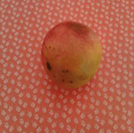
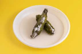
This research used the Fruits and Vegetables dataset from Kaggle10, compiled by Mukhiddinov et al. The dataset contains images of ten types of produce, five fruits (apple, banana, mango, orange, and strawberry) and five vegetables (bell pepper, carrot, cucumber, potato, and tomato). Each type has 2 classes: fresh and rotten, resulting in 20 total categories. A sample fresh mango and rotten okra dataset image are depicted in Fig. 1a and 1b. Images were collected from multiple sources, including other Kaggle datasets such as Fruits-36011 and Fruits Fresh and Rotten for Classification12, as well as public image repositories and search engines. Because the image sources vary, the original dataset contained images with inconsistent dimensions and formats (e.g., JPEG and PNG files). Each image’s folder name acts as its label (e.g., “FreshMango”).
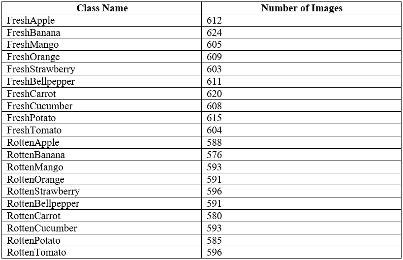
The dataset includes approximately 600 images per class, totaling 12,000 images, and is well balanced across all 20 classes, as seen with the class sizes all being approximately 600 images in Table 1.
Several preprocessing steps were applied to the data, starting with pixel normalization. Each image’s RGB pixel values were rescaled from 0-255 to 0-1 using Keras’ ImageDataGenerator. This normalization prevents any one color channel from disproportionately influencing the model13. All images were then resized to 128 x 128 pixels. This size preserved important visual features while maintaining manageable model input dimensions.
Since the project goal was binary classification, predicting whether produce is fresh or rotten, a new, clean dataset was created. A Python script was used to iterate through the 20 classes, copying each image into either a “fresh” or “rotten” folder, depending on the label prefix. The result was a dataset labeled by freshness status rather than specific fruit or vegetable type.
Data Augmentation and Dataset Splitting
Data augmentation was applied to improve model generalizability and simulate a range of real-world scenarios. Each image was augmented using seven techniques:
- 90 degree rotation
- 270 degree rotation
- Horizontal flip
- Vertical flip
- Random brightness (between 30% darker and 30% brighter) and contrast (between 30% less contrast and 30% more contrast) adjustment
- Added Gaussian noise (change of up to 25 intensity units per pixel)
- Cropping (80% of original height and width) and resizing back to the original size
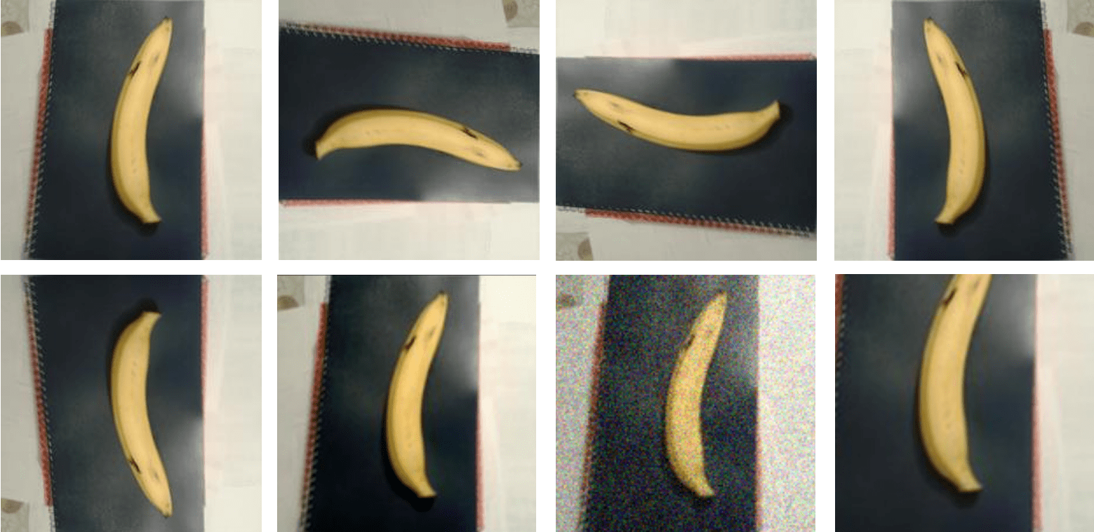
This process generated up to seven images per original image file, as shown with a sample image of a fresh banana in Fig. 2. A small number of images could not be processed due to formatting issues. Before the images were resized when inputted to the model, the mean image dimensions in the augmented dataset were 350px x 300px. In addition, 88% of the images were of the JPEG file type, while the remaining 12% were PNG images. The final augmented dataset contained 95,888 images, achieving a 99.88% augmentation success rate. The 0.12% augmentation failure rate may have been caused by image quality issues such as being partially unreadable (through being saved incorrectly) or having an unsupported color mode for the augmentation procedures, such as CMYK.
The augmented dataset was then randomly split into training, validation, and testing sets, using a 70/15/15 split ratio. This resulted in 67,120 training images and 14,384 validation and testing images. Additionally, all augmentations of a given image remained within a single set to prevent data leakage. The training and validation sets were used consistently across all model training and tuning processes, with the testing set used only for final model evaluation
Model Structure
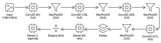
The model used in this research is a CNN model. We chose to use this type of model and neural network due to the known success of CNN models in the past when dealing with computer vision, and specifically in classification from images, as they extract important features from each image in their many layers14.The model consists of 12 total layers, made up of: 4 two-dimensional (2D) convolutional layers, 4 max pooling layers, 1 flattening layer, 1 dense hidden layer, 1 dropout layer, and 1 dense output layer. Fig. 3 demonstrates the basic architecture of the model, with all 12 layers. We built the model using TensorFlow Keras. This 12-layer architecture was selected to balance between overfitting and underfitting, as shallower architectures (e.g., 8 layers) are more prone to underfitting, while deeper architectures (e.g., 16 layers) are more prone to overfitting and increase computational cost without a guaranteed proportional increase in model accuracy15, especially given the size of the dataset used.When an image is passed into the model, it is represented as an array of pixel values.
This array is according to the normalized image size, as each image is 128 pixels high, 128 pixels wide, and has 3 color channels (Red, Green, and Blue). In each convolutional layer, the image is analyzed for features that contribute to the model’s final prediction, and the layer returns a feature map. The max pooling layers after each convolutional layer serve to increase the overall efficiency of the model through decreasing the size of feature maps while still retaining the most important information contained within them. These layers become even more important after later convolutional layers, as the later the convolutional layer is, the more complex the features (and thus the feature maps) become. After the final set of feature maps is returned, the flattening layer converts it from 2D form to a 1D vector so that it is usable in the dense layer, which allows the model to make sense of all the features together and make one final prediction as to whether the given image depicts fresh or rotten produce; a portion of the neurons (the specified dropout rate) are not used in making this prediction, which helps prevent model overfitting16.
The exact output shapes and number of parameters for each layer are shown in Fig. 4 below.
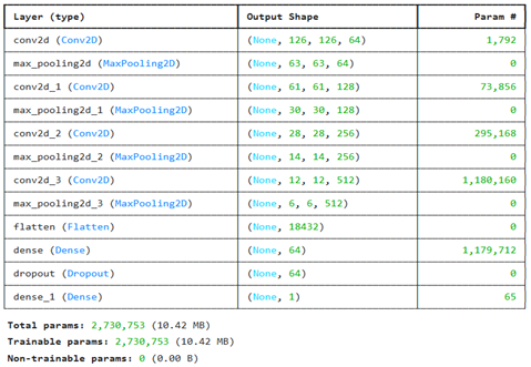
Fig 4 Original model summary (generated using Keras)
Preliminary Testing
Before beginning official model training and tuning, it was important to choose a consistent image resolution to be used with all versions of the model. To do this, we tested and evaluated a baseline model’s performance with five different image resolutions (in px by px): 96 x 96, 112 x 112, 128 x 128, 150 x 150, and 224 x 224. The structure of the model used to test these varying resolutions was the same as the structure in Fig. 4, but it had the following key parametric differences: 32, 64, 128, and 256 filters in the convolutional layers; 128 units in the hidden dense layer; and a dropout rate of 0.5. Each model was compiled using the Adam optimizer (learning rate = 0.001), the binary cross-entropy loss function, and a batch size of 64. Each model was trained for 20 epochs with the implementation of early stopping with a patience of 5 epochs on validation accuracy. Rationale for optimizer and loss function choice as well as training length and early stopping choice is explained further in “Model Training and Tuning.”
Based on the results of these models, the image size used with the best performing model (as judged by validation accuracy) was used to train, validate, and test the original model and transfer learning models discussed later.
Model Training and Tuning
To compile the model, we used the Adam optimizer and the binary cross-entropy loss function. We selected the Adam optimizer due to its consistent high performance across a variety of tasks17. Binary cross-entropy served as the loss function due to its specialization for binary classification with neural networks similar to our CNN model18.
Additionally, training, validation, and testing data generators were created with certain parameters to define the manner in which the model would be trained and tuned. First, the batch size of all the data was set to 64, meaning that the model would process 64 images at a time, then adjust its internal weighting to optimize its accuracy. Also, the class mode for all data was set to binary, directing the data generator to provide binary labels with each image during training (depending on which folder within the dataset contained the image). Finally, the training data generator was instructed to shuffle the order of the images it obtained from the training dataset to create more randomness in the images and reduce the possibility of overfitting; however, the validation data generator was not instructed to do so, so that the model would be evaluated on its accuracy and loss in the same way in each training epoch. The testing generator was created in the same manner as the validation generator; only the images within each were different. None of these parameters was adjusted throughout the training and tuning process.
Each version of the model was trained over 20 epochs (per search trial), and the accuracy metric was used to measure model performance. A training length of 20 epochs was chosen because preliminary runs indicated that performance was maximized well before the last epoch. Early stopping was also implemented with a patience of 5 epochs (based on validation accuracy). The combination of 20 epochs and early stopping mitigated unnecessary computation and run time while still allowing the model to converge. The seven major hyperparameters tuned during the model executions were the number of filters in of the four each convolutional layers, optimizer learning rate, dropout rate, and dense units in the hidden dense layer. The model was tuned using random search with 50 different hyperparameter combinations (trials) and one model execution per trial. In the first convolutional layer, the number of filters as choices for the model were 32 and 64; in the second, they were 64 and 128; in the third, they were 128 and 256; and in the fourth, they were 256 and 512. Optimizer learning rate choices were 0.0005, 0.0001, 0.001, and 0.01. Dropout rate choices were intervals of 0.1 from 0.2 to 0.6, and dense unit choices were 64, 128, 256, and 512.
Saliency Map
A saliency map is a representation of a given image that shows the varying importance of individual pixels to an AI model’s final classification19. The importance of each pixel (also known as its “gradient”) is represented by the color of the pixel on the saliency map. These maps provide helpful information as to the model’s analytical process.
Gradients were calculated using TensorFlow’s GradientTape API. Additionally, the map color was set so that brighter pixels signified stronger gradient while darker pixels signified weaker or no gradient. A random image was selected from the validation data and input into the model for classification. Subsequently, its saliency map was generated.
Transfer Learning Model Training and Tuning
To provide direct comparison with the original model proposed in this research, we also trained and tuned two prominent transfer learning CNN architectures: ResNet50 and MobileNetV220. Both architectures were pre-trained using ImageNet weights and tuned using random search with 20 different hyperparameter combinations (trials) and one model execution per trial. The hyperparameters manipulated were: optimizer learning rate (0.0005, 0.0001, 0.001, and 0.01) and dropout rate (intervals of 0.1 from 0.2 to 0.6). All other training and tuning components were kept the same as in the experiment with the original model, including the optimizer, loss function, batch size, training data generator, validation data generator, training length, and early stopping protocols.
Results
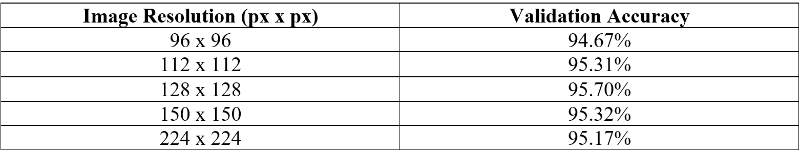
Table 2 summarizes the results of the baseline model with different image resolutions in terms of validation accuracy (see definition under Table 3). As seen, the image resolution that corresponded to the best baseline model performance was 128px x 128px. Thus, this resolution was used for the remainder of the training, tuning, and testing process. This resolution may have had the highest performance as it provides a balance between visual detail and model complexity, maintaining the most important parts of many images for the model to classify while omitting unnecessary portions.
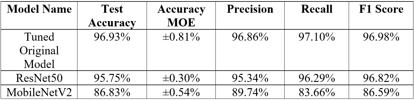
Table 3 summarizes the results of the tuned original CNN model and the transfer learning models in terms of accuracy (with their margin of error), precision, recall, and F1 score. Accuracy is simply the number of correct predictions each version of the model made divided by the total number of predictions it made. Precision is calculated similarly; however, instead of considering all correct predictions and total predictions, it only considers predictions made for a certain class. In other words, it is the accuracy when predicting each class individually. Recall, on the other hand, measures correct predictions of a certain class divided by the total number of instances of the class in the testing data. The precision and recall values in the table are averages of their respective model versions’ precision and recall for each target class (fresh and rotten). Finally, the F1 score balances these two metrics as it is the harmonic mean of the two21. Additionally, the margin of error (MOE) for test accuracy with 95% confidence was computed using non-parametric bootstrap resampling22 with replacement 1,000 times.
The tuned original model performed the best out of the three models over all metrics, with a statistically significant improvement in test accuracy compared to the two transfer learning models. Of the two transfer learning models, ResNet50 performed noticeably better than MobileNetV2, having an average of 9.35% greater performance over all the metrics. In terms of precision, recall, and F1 score, the tuned original model’s values were high and mostly balanced, indicating that it performed consistently in identifying fresh versus rotten images (with minimal bias toward either class). ResNet50 had slightly lower but comparable values, indicating that it was also mostly consistent and minimally biased toward certain classes. However, MobileNetV2 had significantly lower recall (83.66%) compared to its precision (89.74%), which reveals that it likely misclassified a higher portion of the rotten images than the fresh images. This bias toward wrongly classifying a significant amount of images as fresh may be due to its failure to recognize certain fine texture patterns during feature extraction, such as minor bruising or discoloration.
Training Curves

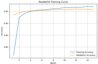
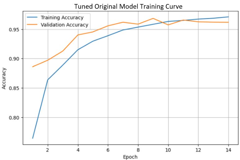
Training curves for all three models were generated for the three different final model versions after training and tuning (i.e., using their final best weights). Fig. 5a and 5b indicate that the tuned original model and ResNet50 show general convergence between their training accuracy and validation accuracy, as the curves appear to plateau around their maximal values. Fig. 5c reveals that MobileNetV2, on the other hand, shows significant overfitting. This is because its training accuracy continues to increase while its validation accuracy plateaus at a significantly lower value23. These results underscore the success of the tuned original model and ResNet50, as these models were able to successfully generalize their training to the validation data.
Confusion Matrix
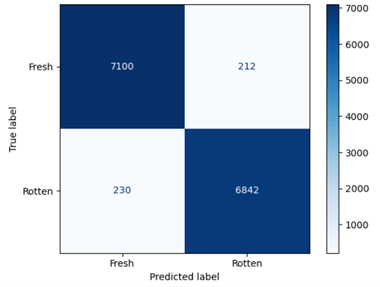
The confusion matrix for the tuned original model in Fig. 6 compares the true data labels (the labels of the actual testing data) and the predicted labels (the labels the model predicted on the same data). Of the 7,312 images of fresh produce given to the model, it classified 7,100 images correctly and 212 images incorrectly. Of the 7,072 images of rotten produce given to the model, it classified 6,842 images correctly and 230 images incorrectly.
The confusion matrix reveals that the model makes a slightly higher percentage of errors on rotten produce (3.25%) than on fresh produce (2.90%). This may be due to there being slightly more training images for the fresh class than the rotten class. Closer examination revealed that the variability of the error percentages can also be attributed to the rotten class having greater classification difficulty than the fresh class in specific cases. Many of the rotten images that the model failed to recognize were with fruits in uneven lighting, such as with shadows or glare, which distorted the color patterns the model was trained to recognize. The lighting conditions in these images dampened or brightened discolored/decayed areas of the fruit, making them appear similar to their appearance for fresh produce. The model’s failure to recognize the color patterns in the misclassified rotten images is likely a result of there not being a significant amount of similar images in the training images.
ROC and PR Curves
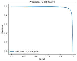
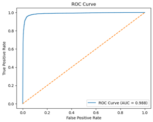
The ROC and Precision-Recall curves with AUC for the tuned original model (on the test images) are shown. Fig. 7a compares the true positive rate (the rate at which the model correctly predicted that an image was fresh) with the false positive rate (the rate at which the model incorrectly predicted that an image was fresh)24. On the other hand, Fig. 7b compares the model’s precision and recall. Both curves use different probability threshold values to obtain the values shown; by default (for true model prediction) the threshold is 0.5, but it is manipulated to gauge model confidence in order to generate ROC and Precision-Recall curves. AUC is simply the area under each curve, with a higher AUC (i.e., closer to 1) corresponding to better general classification success25.
The ROC curve lies close to the upper-left corner of Fig. 7a, with an AUC of 0.988, indicating that it is largely able to distinguish between fresh and rotten produce with high confidence. The curve remains far above the orange dashed line, which represents the model’s ROC curve if it were classifying the images purely based on random chance. Similarly, the Precision-Recall curve demonstrates great class discrimination with great confidence, as the curve lies close to the upper-right corner of Fig. 7b and has an AUC of 0.989.
Saliency Maps
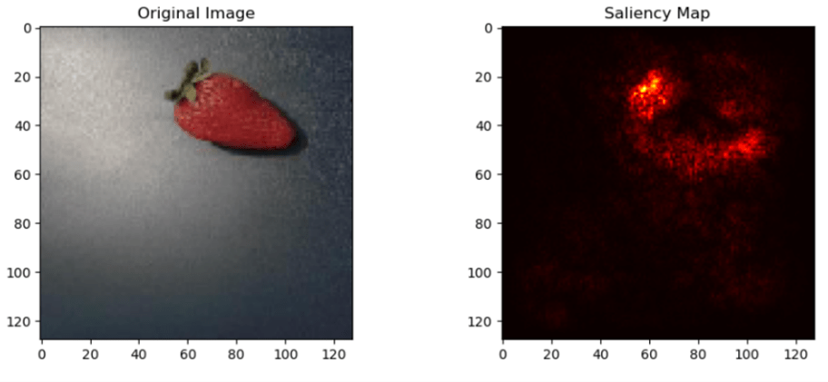

The saliency maps demonstrate the model’s ability to identify distinguishing features that make produce appear fresh or rotten. In Fig. 8a, most of the bright pixels (i.e., the ones that are not black) are in the same area of the saliency map as the red, glossy, uniform surface near the top of the original strawberry. In contrast, in Fig. 8b, most of the bright pixels correspond to the most severely bruised or darkened region of the original rotten strawberry. This is similar to how a human freshness inspector would have gauged whether the fruit is fresh or rotten, as the portion of the fresh strawberry that best indicates its freshness is the area with consistent, deep red color, while the portion of the rotten strawberry that best indicates its rottenness is the discolored area.
Discussion and Conclusion
The notable changes from the baseline model to the tuned original model were that the number of filters in the four convolutional layers increased from 32, 64, 128, and 256 originally to 64, 128, 256, and 512; the dense units in the hidden layer decreased from 128 to 64; and the learning rate for the Adam optimizer decreased from 0.001 to 0.0005. The dropout rate remained the same as the rate for the baseline model, 0.5. Increasing the number of filters in all the convolutional layers likely increased model performance because it allowed the model to recognize more complex feature patterns in the images. For example, fine texture patterns may have not been recognized to as great an extent with the original number of convolutional filters in each layer. On the other hand, decreasing the number of dense units in the hidden dense layer helped to mitigate model overfitting by decreasing the number of parameters involved in decision-making26. Additionally, decreasing the optimizer learning rate allowed for finer internal model weight adjustments, helping to avoid overadjustment and oscillation in accuracy and loss.
The high performance of the tuned CNN model used in this research indicates that it is able to effectively compare various features of fruits and vegetables as a basis for their freshness/rottenness classification. It can also achieve competitive accuracy with other state-of-the-art transfer learning models such as ResNet50 and MobileNetV2. Thus, our hypothesis that an original, non-transfer learning CNN model can accurately classify fresh and rotten produce (and compete with transfer learning architectures for the same task) was confirmed. The dataset used and its augmentation may have been largely responsible for the model’s success, as it was balanced and captured many different conditions of produce, such as varying orientation and lighting.
Despite its high performance, the research has some limitations that must be considered. First, the dataset is limited to 10 different types of produce, not accounting for the many other different types, which could be expanded on. In addition, the fact that the model only classifies produce as fresh or rotten may oversimplify quality classification, considering the existence of other classifications such as ripe and overripe. Finally, the model was tested with the same architecture over all executions, and the performance of other original models with different architectures (outside of the two transfer learning model architectures tested) remains largely unseen.
Given the model’s high performance, it may be applicable to real-world contexts such as in households and food retail businesses. In households, the model could be integrated into a mobile application. Users could take photos using their mobile phone cameras, and the images would be run through the model. The model would then return whether the produce in the picture is fresh or rotten. In this application, however, there must be a check that occurs before inputting the image to the model. This check must ensure that the photo is of good enough quality for the model and that it actually contains a fruit or vegetable of the types represented in the model. This functionality could be enabled through the use of an external API that detects specific produce types, such as the Google Cloud Vision API. Regarding the model’s applicability in food retail businesses, a practical use would be in real-time produce spoilage detection. If cameras were positioned in stores where they could take periodic pictures of produce, these pictures could be run through the model, and spoiled produce could be removed. In addition, amounts of fresh and spoiled produce could be reported to business managers, allowing them to optimize their buying habits to ensure most or all of their purchased produce is sold and little to none goes to waste through spoilage. However, these applications are tentative, as the model has only shown strong performance in a controlled, experimental setting and has not been tested in real household or retail environments.
Additional testing would be needed before the model could be deemed applicable and trustworthy for use in these real-world environments. This future work could focus on increasing the scope of the model’s awareness. The scope could be increased through experiments training, validating, and testing the model on a dataset containing a wider variety of produce (e.g., lettuce, spinach, and onions) or types of classification (e.g., fresh, ripe, overripe, and spoiled). These implementations would better reflect real-world scenarios where there is often the need for classification of many different types of produce (not just the 10 types used in the dataset in this study) and more specific freshness detection (not only fresh and rotten). Further future work could prepare the model for use under real-world lighting conditions and camera setups by testing it with the manipulation of prospective setups.
In conclusion, although the model in this study was highly successful, there is still room for improvement, both in this model and in the topic of food waste mitigation as a whole. However, this research demonstrates the applicability of deep learning models to everyday tasks, not only to drive efficiency but also sustainability and more environmentally friendly consumption.
Acknowledgments
The author thanks John Basbagill (Stanford University, PhD) for his mentorship and guidance throughout the research process.
References
- United Nations Environment Programme (2024). Food waste index report 2024. https://www.unep.org/resources/publication/food-waste-index-report-2024. [↩] [↩] [↩]
- Food and Agriculture Organization of the United Nations, International Fund for Agricultural Development, UNICEF, World Food Programme, & World Health Organization (2024). The state of food security and nutrition in the world 2025—Addressing high food price inflation for food security and nutrition. FAO. https://doi.org/10.4060/cd6008en. [↩]
- Widayat, W., Handayanto, E., Irfani, & A.D., Masudin, I. (2025). A systematic literature review and future research agenda on the dynamics of food waste in the context of consumer behavior. Sustainable Futures, 9. https://doi.org/10.1016/j.sftr.2025.100491. [↩]
- Khan, M. S. A., Husen, A., Nisar, S., Ahmed, H., Muhammad, S. S., & Aftab, S. (2024). Offloading the computational complexity of transfer learning with generic features. PeerJ Computer Science, 10, Article e1938. https://doi.org/10.7717/peerj-cs.1938. [↩]
- D. Ulucan, O. Ulucan, & M. Turkan (2019). A comparative analysis on fruit freshness classification. 2019 Innovations in Intelligent Systems and Applications Conference (ASYU), 1-4. https://doi.org/10.1109/ASYU48272.2019.8946385. [↩]
- M.A. Sofian, A.A. Putri, I.S. Edbert, & A. Aulia (2024). AI-based recognition of fruit and vegetable spoilage: Towards household food waste reduction. Procedia Computer Science. 245, 1020-1029. https://doi.org/10.1016/j.procs.2024.10.330. [↩]
- M. Mukhiddinov, A. Muminov, & J. Cho (2022). Improved classification approach for fruits and vegetables freshness based on deep learning. Sensors. 22(21), 8192. https://doi.org/10.3390/s22218192. [↩]
- Yang, C., Guo, Z., Barbin, D. F., Dai, Z., Watson, N., Povey, M., & Zou, X. (2025). Hyperspectral imaging and deep learning for quality and safety inspection of fruits and vegetables: A review. Journal of Agricultural and Food Chemistry, 73(17), 10019–10035. https://doi.org/10.1021/acs.jafc.4c11492. [↩]
- Liu, Y., Wei, C., Yoon, S. C., Ni, X., Wang, W., Liu, Y., Wang, D., Wang, X., & Guo, X. (2024). Development of multimodal fusion technology for tomato maturity assessment. Sensors, 24(8), 2467. https://doi.org/10.3390/s24082467. [↩]
- M. Mukhiddinov (2022). Fruits and vegetables dataset. https://www.kaggle.com/datasets/muhriddinmuxiddinov/fruits-and-vegetables-dataset. [↩]
- M. Oltean (2017). Fruits-360 dataset. https://www.kaggle.com/datasets/moltean/fruits. [↩]
- S.R. Kalluri (2017). Fruits fresh and rotten for classification. https://www.kaggle.com/datasets/sriramr/fruits-fresh-and-rotten-for-classification. [↩]
- Winarno, S., Alzami, F., Naufal, M., Al Azies, H., Soeleman, M. A., & Ahamed Hassain Malim, N. (2025). EfficientNet-KNN for real-time driver drowsiness detection via sequential image processing. Ingenierie des Systèmes d’Information, 30(7), 1703–1713. https://doi.org/10.18280/isi.300703. [↩]
- Krichen, M. (2023). Convolutional neural networks: A survey. Computers, 12(8), 151. https://doi.org/10.3390/computers12080151. [↩]
- Chen, F., & Tsou, J. Y. (2022). Assessing the effects of convolutional neural network architectural factors on model performance for remote sensing image classification: An in‑depth investigation. International Journal of Applied Earth Observation and Geoinformation, 112, Article 102865. https://doi.org/10.1016/j.jag.2022.102865. [↩]
- I. Azuri, I. Rosenhek-Goldian, N. Regev-Rudzki, G. Fantner, & S.R. Cohen (2021). The role of convolutional neural networks in scanning probe microscopy: a review. Beilstein Journal of Nanotechnology, 12, 878-901. https://doi.org/10.3762/bjnano.12.66. [↩]
- R.M. Schmidt, F. Schneider, & P. Hennig (2021). Descending through a crowded valley—benchmarking deep learning optimizers. International Conference on Machine Learning, 139,9367-9376 (2021). https://doi.org/10.48550/arXiv.2007.01547. [↩]
- Tsoi, N., Candon, K., Li, D., Milkessa, Y., & Vázquez, M. (2020). Bridging the gap: Unifying the training and evaluation of neural network binary classifiers. arXiv. https://doi.org/10.48550/arXiv.2009.01367. [↩]
- Amorim, J. P., Abreu, P. H., Santos, J. A. M., Cortes, M., & Vila, V. (2023). Evaluating the faithfulness of saliency maps in explaining deep learning models using realistic perturbations. Information Processing & Management, 60(2), Article 103225. https://doi.org/10.1016/j.ipm.2022.103225. [↩]
- Baumgartl, H. & Buettner, R. (2021). Developing efficient transfer learning strategies for robust scene recognition in mobile robotics using pre‑trained convolutional neural networks. arXiv. https://doi.org/10.48550/arXiv.2107.11187. [↩]
- J.C. Obi (2023). A comparative study of several classification metrics and their performances on data. World Journal of Advanced Engineering Technology and Sciences, 8(1), 308-314. https://doi.org/10.30574/wjaets.2023.8.1.0054. [↩]
- Efron, B. (1987). Better Bootstrap Confidence Intervals. Journal of the American Statistical Association, 82(397), 171–185. https://doi.org/10.1080/01621459.1987.10478410. [↩]
- Salman, S., & Liu, X. (2019). Overfitting mechanism and avoidance in deep neural networks. arXiv. https://doi.org/10.48550/arXiv.1901.06566. [↩]
- Obuchowski, N. A. (2003). Receiver operating characteristic curves and their use in radiology. Radiology, 229(1), 3–8. https://doi.org/10.1148/radiol.2291010898. [↩]
- Li, J. (2024). Area under the ROC Curve has the most consistent evaluation for binary classification. PLOS One, 19(12), e0316019. https://doi.org/10.1371/journal.pone.0316019. [↩]
- Baumgartl, H. & Buettner, R. (2021). Developing efficient transfer learning strategies for robust scene recognition in mobile robotics using pre‑trained convolutional neural networks. arXiv. https://doi.org/10.48550/arXiv.2107.11187. [↩]


