Classifying Marine Mammals Using Convolutional Neural Networks

Abstract

Deep learning continues to advance image recognition capabilities rapidly, providing cutting-edge support for wildlife conservation initiatives. In this study, we develop a Convolutional Neural Network (CNN) framework to distinguish individual whales and dolphins extracted from the Happywhale dataset, demonstrating high precision in marine mammal identification. Our model achieves robust feature extraction and enhanced class separability by leveraging an EfficientNetB5 backbone with an ArcFace loss function. Multiple data augmentation techniques, including random cropping, grayscale conversion, and color manipulation, are used to improve the model’s adaptability across various imaging conditions. We incorporate a k-nearest neighbors (KNN) algorithm at the inference stage to refine predictions, especially when assigning labels to new individuals. By combining these strategies, we were able to boost classification accuracy, reaching a Mean Average Precision at 5 of 0.88. The results show how effective deep learning can be for fine-grained image identification tasks in marine mammal conservation. Beyond accuracy, the model offers real potential to simplify research workflows and support long-term conservation efforts for marine life.

Keywords: Marine Mammal Identification, Convolutional Neural Network (CNN), Deep Learning, EfficientNetB5, ArcFace, Data Augmentation, K-Nearest Neighbors (KNN), Wildlife Conservation, MAP@5, Population Tracking

1. Introduction

Identifying and classifying individual marine mammals is critical for research on marine mammal conservation efforts and population tracking. Traditional identification methods typically rely on manual photo matching, which is time-consuming and prone to human error. Artificial intelligence and machine learning offer methods to accurately identify marine mammals without these downsides

Identifying and classifying individual marine mammals is critical for research on marine mammal conservation efforts and population tracking. Traditional identification methods typically rely on manual photo matching, which is time-consuming and prone to human error. Artificial intelligence and machine learning offer methods to accurately identify marine mammals without these downsides¹.

This research leverages the Happywhale dataset, which comprises tens of thousands of labeled images representing over 15,000 unique marine mammal individuals across 30 distinct species. The goal is to create a model capable of effectively and reliably distinguishing individual animals based on physical features such as fluke shape, skin patterns, and body size. This study leverages a pre-trained EfficientNetB5 backbone as the feature extractor and integrates an ArcFace loss layer to enhance model performance by maximizing the separation between classes (i.e., individuals).

Additionally, this research explores various image augmentation techniques to improve the model’s generalization ability. This study demonstrates the potential of deep learning for wildlife monitoring and establishes a practical and scalable framework for similar applications where technology meets biology.

2. Background

The Happywhale dataset is a whale and dolphin identification challenge comprising over 51,000 labeled images representing 15,587 unique marine mammals from more than 30 different species. These images were collected through contributions from marine researchers and photographers supporting the identification, tracking, and conservation of marine mammal populations worldwide. Whales and dolphins are typically recognized by their distinct features such as fluke shape, dorsal fin markings, skin patterns, and shape². Manually classifying images of marine mammals can be difficult and time consuming, and this issue gets larger as datasets increase in size.

Identifying marine mammal species is essential to understanding their populations, social dynamics, and migration routes. Each marine mammal exhibits unique physical features, such as markings or scars, which can serve as visual identifiers. Traditionally, scientists have collected photographs of these markings and manually matched them to existing records. Although this manual photo identification method has proven effective, it is often time-consuming and expensive. As researchers gather larger datasets, the potential for human error increases, making it difficult to maintain accuracy. Additionally, this manual process can create significant delays in data analysis, which can be critical when monitoring the health of marine ecosystems and the effect of environmental changes³. Identifying individuals is challenging due to subtle variations in markings, environmental factors, and image quality, making machine learning models crucial for use in the real world.

The primary objective of this study is to develop a model that can accurately and reliably classify individual whales, dolphins, and other marine animals within the Happywhale dataset. This high-performance identification model will support marine biologists and conservationists in tracking marine mammal populations. The approach utilizes modern machine learning techniques, such as transfer learning and data augmentation. These methods allow the model to handle the complexity and unpredictability of real-world images.

This research fills a gap in marine animal conservation by developing an automated and scalable approach to identify individuals. The methods used in this study are designed to achieve high accuracy and provide a practical tool for conservationists, contributing to the conservation efforts of marine mammals worldwide.

3. Methodology

The methodology of this study involves developing the best possible deep learning model to classify whale and dolphin images into specific categories. The model’s design and training processes were optimized to enhance accuracy and generalizability. Transfer learning, loss functions, and various data augmentation techniques were also used to improve model performance. Here are the key components used to set up the model:

The model uses EfficientNetB5 as its backbone. EfficientNetB5 is a convolutional neural network that strikes a balance between accuracy and efficiency, ensuring the model runs promptly while minimizing the sacrifice of accuracy. The EfficientNetB5 model efficiently scales the neural network across three dimensions:

1. Depth Scaling: This increases the depth of training data, allowing the model to learn subtle patterns in images. This enables the model to learn from more complex, layered data. However, overusing this method may lead to higher computational demands and a decline in efficiency.
2. Width Scaling: This method of scaling adds more neurons to each layer of the model, expanding its width. As a result, the CNN can learn more nuanced patterns in data. Depth and width scaling work in harmony to effectively extract features from data.
3. Resolution Scaling: The EfficientNetB5 model scales images in a balanced manner, ensuring that images are high-quality and that nuanced features can be extracted while maintaining a decent level of computational demand⁴.

The ArcFace loss layer is introduced as the classification head for this model. ArcFace increases the separation between different classes, improving the model’s ability to distinguish images. It achieves this by introducing Additive Angular Margin Loss to the feature vectors. This additional margin in ArcFace creates a more robust distinction between image classes. This enhanced the model’s discriminative learning and accuracy in identifying images across a large subset of classes. The loss layer operates by normalizing each feature and then using a cosine similarity metric for each feature. Then, ArcFace makes it easier to distinguish between classes by adding a fixed angle, or angular margin, between the feature vector and the target class. This contributes to making class boundaries more distinct, enforcing a distinct separation between classes⁵.

3.1 Architecture Selection Rationale

Prior to selecting EfficientNetB5 as our backbone architecture, experiments were conducted to compare multiple models on their inference capabilities on the Happywhale dataset. Each model was evaluated for Cloud inference using Tensor Processing Units (TPUs), accuracy on fine-grained image classification tasks, and memory utilization on high resolution inputs. EfficientNetB5 achieved the best overall balance between computational efficiency, attention to detail, and accuracy, and was therefore selected for this task.

EfficientNetB5 was compared against several baseline architectures, including ResNet50, EfficientNetB3, EfficientNetB5, and EfficientNetB7. The selection of EfficientNetB5 was based on its balance between accuracy and computational cost. Specifically, EfficientNetB5 demonstrated superior feature extraction capabilities and reasonable computational demand compared to other models when tested on the Happywhale dataset.

3.2 Data Preparation and Augmentation

Kaggle’s Happywhale dataset is split into training and testing sets. A CSV file containing the filename for each image and its corresponding label is included. Some labels include: (bottlenose_dolphin), (beluga), (killer_whale), (blue_whale), and many others. We put each image through a series of transformations to improve the model’s ability to process and develop an understanding of the features in the images. The key transformations that the images undergo include:

• Random Cropping: Images are cropped randomly using full-body, YOLOv5, Detic, or Vision Transformer. This allows the model to focus on specific body parts of the whale or dolphin.
• Color Adjustments: Hue, saturation, contrast, and brightness are randomly altered to allow the model to handle various lighting and color conditions effectively.
• Grayscale Conversion: Converting images to grayscale enhances the model’s ability to recognize patterns based solely on pixel intensity values.

Flowchart-style architecture diagram of the EfficientNetB5 model with ArcFace loss function. The flowchart begins by performing image augmentations on training data, creates a model, and finally runs to make predictions, which are exported to a CSV format and submitted.

3.3 Data Splitting and Leakage Prevention

Kaggle distributes the dataset in two completely separate folders in the Happywhale competition. The first, train_images/, is accompanied by a train.csv file that lists the species and individual_id for every training photo. The second, test_images/, contains unlabeled images. While some individuals that appear in the test set can be absent in the training data, no image in the training folder is duplicated in the test folder. This organizer-enforced separation and organization of images eliminates the risk of leakage between the two data folders.

3.4 Class Imbalance Analysis

The Happywhale training dataset exhibits severe class imbalance across species, with bottlenose dolphins representing 9,664 images while species such as Fraser’s dolphins contain only 14 images. Image classes such as the Killer Whale are in the middle of the pack, representing 962 images in the training dataset.

The species distribution follows a pattern commonly seen in real-world ecological datasets. The top five most common species account for 64.7% of all images, while the bottom 10 species collectively represent less than 3% of the dataset. Individual-level imbalance is even more pronounced, with some individuals appearing in hundreds of images while others have only a single instance⁶.

Species distribution within the Happywhale dataset.

Species	Image Count
bottlenose_dolphin	9 664
beluga	7 443
humpback_whale	7 392
blue_whale	4 830
false_killer_whale	3 326
dusky_dolphin	3 139
spinner_dolphin	1 700
melon_headed_whale	1 689
minke_whale	1 608
killer_whale	1 493
fin_whale	1 324
gray_whale	1 123
bottlenose_dolphin	1 117
killer_whale	962
southern_right_whale	866
spotted_dolphin	490
sei_whale	428
short_finned_pilot_whale	367
common_dolphin	347
cuviers_beaked_whale	341
pilot_whale	262
long_finned_pilot_whale	238
white_sided_dolphin	229
brydes_whale	154
pantropic_spotted_dolphin	145
globis	116
commersons_dolphin	90
pygmy_killer_whale	76
rough_toothed_dolphin	60
frasers_dolphin	14

3.5 Imbalance Mitigation Strategy

Our approach to handling the severe class imbalance combines several complementary techniques rather than relying on traditional oversampling methods. The implementation addresses imbalances at multiple stages of the model creation pipeline:

1. Cross-validation Based Data Splitting: We implemented a 10-fold cross-validation strategy that ensures balanced representation across each fold while maintaining the natural distribution within each fold. This approach helps prevent overfitting to overrepresented classes during training and provides more robust performance across groups with different frequencies in the dataset.
2. Augmentation-based Minority Class Enhancement: Rather than using traditional oversampling methods, we applied data augmentation techniques, such as random horizontal flipping and others, across all classes. This strategy indirectly benefits minority classes by increasing their effective representation through transformations while preserving biological features critical for species identification⁷.
3. Natural distribution preservation: Maintaining original class distribution during training was feasible because natural encounter frequencies present in the training dataset contain valuable ecological information. Artificially balancing the training dataset can disrupt learned patterns that reflect real-world probabilities.

3.6 Training Strategy

Training occurred on a Tensor Processing Unit (TPU) on Kaggle, significantly reducing training times for this model while utilizing fewer resources. The batch size is set to 16 * the number of TPU replicas, leveraging Kaggle’s TPUs.

Runtime Benchmarks

On Kaggle, the EfficientNetB5 + ArcFace notebook finished all 30 training epochs in 1 hour 15 minutes on a single TPU v3-8 instance. On the other hand, running the same code, adapted for Kaggle’s NVIDIA P100 16 GB GPU, required 4 hours and 7 minutes. Therefore, the TPU accelerator delivers about a 3.3-fold increase for this workload, showcasing the benefits of TPU usage over GPUs.

Free Research Tier

Kaggle grants every user up to 9 hours a day of TPU v3-8 usage at zero cost, so all experiments required in this study were conducted free of charge⁸.

3.7 K-Nearest-Neighbor Head

A soft-max layer assumes a set of labels, yet about 10 % of Happywhale test images belong to individuals not present in the training dataset. The KNN head is primarily used in the EfficientNetB5 + ArcFace model. After the CNN produces a 512-dimensional feature vector, a -Nearest-Neighbor (KNN) search is used to decide the final⁹.

For each query to the KNN head, the model performs four steps:

1. Run the image through the CNN and take the 512-dimensional feature vector that is generated right before the ArcFace head.
2. Normalize the vector by dividing it by its own magnitude. As a result, the vector will have a value of 1. This results in the dot product of two vectors being equal to their cosine similarity.
3. Use cosine distance to fetch the closest training embeddings.
4. Use scikit-learn’s NearestNeighbors to find the k closest training vectors. This takes about 14 milliseconds on a single CPU core.
5. Finally, the KNN head counts how many times each label appears among its neighbors. The label that appears the most commonly is the prediction. If a tie occurs, the label with the shortest inverse distance is chosen.
6. If the nearest neighbor has a cosine distance greater than , we output the special label new_individual. The cosine distance of 0.62 was chosen because it maximized MAP@5 by accurately assigning the new_individual label.

3.8 Hyper-parameter Selection for k

A grid search on the validation fold with shows performance peaking at .

was chosen because smaller values resulted in instability among minority classes, and larger values added distractors to predictions.

3.9 Distance-based Thresholds for new_individual

Let be the distance to the closest neighbor and define a confidence .
A grid search found that if the safest choice is to output the special label new_individual. This allowed a balance between false positives of assigning the label new_individual to an image while ensuring this label is not overused.

3.10 Ensemble and Blending

The final model predictions are generated using a blending strategy that combines the performances of multiple models, which range across several different epochs and crop augmentations. Snapshots were also taken and used throughout the model’s training. These checkpoints were combined using optimized weights to enhance the model’s performance. Optimized weights were also used for each model in the ensemble to ensure that the score produced by the ensemble is maximized¹⁰. The following equation represents this:

   

where represents the weight assigned to model and is its prediction. The complete implementation of our ensemble blending strategy, including a model training notebook and weight selection, is available at https://github.com/adityapkatre/Research.

Model Selection Criteria

Thirty candidate checkpoints were first shortlisted from a pool of 120 training runs by applying two filters on their out-of-fold predictions:

• A minimum MAP@5 of 0.840 on the 5-fold validation split that keeps each individual_id in a single fold
• Five specialist models trained only on beluga, back fin, or full-body crops were included in the blend, even if they scored a lower MAP@5 in isolation. This helps reduce errors made by models that took a more holistic approach to classifying certain species.

This resulted in a total of 30 reasonably strong yet diverse sets of predictions, each one stored as a .csv file.

Weight Optimization

Let () be the rank assigned by model (j) to identity (i).
Ranks are converted to base scores with the monotone lookup (w(r)={10, 6.5 ,3.3 ,2.9 ,2.7}).
The ensemble score for an identity is calculated using the following equation:

   

where (f_i) is the number of training photos of that individual, and where the special label new_individual is down-weighted by 4 unless it is ranked first or second to keep its false-positive rate in check.

The coefficients () were learned with a greedy coordinate-ascent search on the same 5-fold split:

1. Initialize all ().
2. For each model, (j), evaluate the MAP@5 on the out-of-fold data after changing () by (), while keeping the modification that improves the MAP@5 by at least .
3. Repeat step 2 until a full sweep over all (j) yields no improvement greater than MAP@5.

Starting from the all-ones vector, this coordinate search converged in under three minutes and produced the final weight vector:

   

When these weights are applied to the 30 OOF prediction files, the blended submission scores MAP@5 = 0.88 ( 0.002 across folds), a +2.8 point gain over the best single checkpoint.

3.11 Model Architectures and Code Excerpts

To ensure reproducibility and demonstrate the complexity of the models, the following figures show snippets of the TensorFlow/Keras code and Matplotlib graphs used for training each model, embedded as code listings. These snippets provide an overview of the layers, data preprocessing steps, and training loops employed.

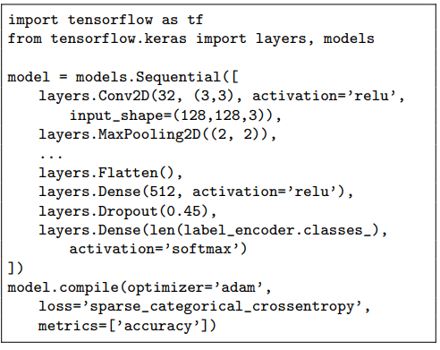
Implementation of the Basic CNN model architecture using TensorFlow/Keras. The model comprises several convolutional layers that extract features from images, along with various augmentation methods to enhance feature extraction and improve model performance.

This first model’s simplistic architecture and relatively short training regime resulted in the lowest scores among the four tested models for the Happywhale dataset.

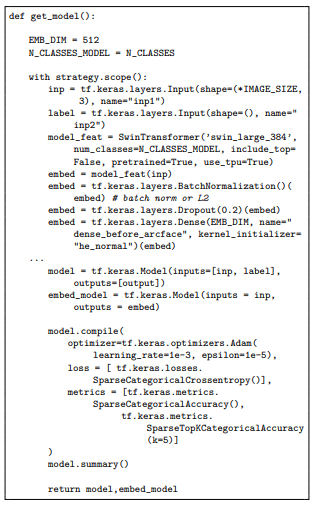
Python function get_model(), which builds the training network. It adds a batch normalization, dropout, and a 512-D dense layer before compiling with Adam, specifying a learning rate, and ensuring that the top-5 accuracy metrics are provided.

Learning rate schedule employed during model training. The x-axis represents training epochs (0-30), and the y-axis represents the learning rate (x10^-5). The graph displays three separate phases of training: (1) warm-up phase (epochs 0-6) with an almost linear increase from 1×10^-6 to 8×10^-5, (2) brief sustain phase at maximum learning rate, and (3) exponential decay phase (epochs 6-30) that ultimately reaches 1×10^-6. The schedule increases stability of initial training while preventing overfitting in later epochs, allowing the model to be more fit for real-world scenarios represented in the dataset. The graph illustrates a learning rate schedule employed during the training process of the model with an EfficientNetB5 backbone. After a brief warm-up phase, the learning rate rises sharply to a peak, the gradually decreases as training progresses. The learning rate (y-axis) initially follows a warm-up phase, which is quickly followed by a peak. As the number of epochs (x-axis) increases, the learning rate gradually decays, which results in the optimization of the model.

The model blend, as illustrated by the integrated blending and augmentation strategies in the code snippet below, achieved the highest MAP@5 score of 0.88. The difference in MAP@5 score is subtle but significant due to the refinement of inference strategies and data handling.

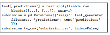
Implementation of the ensemble blending strategy that combines predictions from checkpoints of several independent models. The blender function uses outputs from 30 model variants to produce final predictions, achieving the highest MAP@5 of 0.88.

The blending approach shown in the code snippet above uses predictions from various models to produce more accurate predictions. This shows how multiple models working in combination can lead to improved overall production quality.

In summary, the four models showcased progressed from a relatively simple CNN with a score of 0.10 to a high-performing, blended solution that achieved a score of 0.88, which is higher than other baselines showcased in Table 3. These results represent the outcome of creating several iterations and improvements in making predictions in challenging, fine-grained datasets.

3.12 Evaluation Metrics

The primary evaluation metric used in the Happywhale competition on Kaggle is the Mean Average Precision at 5 (MAP@5). This metric is specifically designed to measure the quality of a model’s top-five predictions for each image in the test set, thereby assessing how effectively the model prioritizes correct labels at the highest ranks. By limiting the evaluation to the top five predictions per image, MAP@5 focuses on the model’s ability to accurately pinpoint the correct individual from a shortlist of candidates, rather than requiring it to produce a perfectly ordered, full-length ranking. Such a constraint reflects practical scenarios in which only the top few suggestions are most important, such as identifying a specific whale or dolphin from a large database.

Additionally, MAP@5 is applied consistently to both validation and test sets, ensuring that the metric used during model tuning and selection is the same as that used in the final evaluation. This consistency fosters reliable model comparison and supports a more robust understanding of how well the model can generalize to new, unseen images.

To define MAP@5 more concretely, let ( U ) be the total number of images in the test (or validation) set, and for each image, assume the model produces ( n ) predicted labels ranked from most to least likely. The value ( k ) represents the position (or cutoff) in the ranked list, with ( ), since we only consider the top five predictions. For each image ( ), we denote its correct label as a “relevant” item. The model’s task is to place this relevant label as high as possible among its predicted labels.

We define a relevance function ( ), which equals 1 if the correct label is found at rank ( k ) and 0 otherwise. The precision at cutoff ( k ), denoted ( P(k) ), is computed as the fraction of correct labels among the top ( k ) predictions:

   

.

Since only one correct label exists per image (under the assumption that each image corresponds to a single individual), any rank ( k ) beyond the first occurrence of the correct label does not contribute additional precision improvements.

The MAP@5 metric is then calculated by summing the precision values at each cutoff ( k ) where the correct label is found and then averaging this quantity across all images. Formally, if we let ( n ) be the number of predictions for each image, and consider only up to ( ) predictions for MAP@5, the formula can be expressed as:

   

In this formula, (U) represents the number of images, (P(k)) represents the precision at cutoff (k), (n) is the number of predictions per image, and indicates whether the item at rank (k) is a correct label if the item is an incorrect label, the is set to zero.

Once an image is labeled correctly, it’s marked as “found” and is no longer considered in the evaluation. On the other hand, if the model predicts the correct label multiple times in a row for a given image, only the first prediction counts for the (MAP@5) evaluation, and the rest are dropped.

To illustrate this with a simple example, consider a single image with the correct label “A.” Suppose the model’s top five predictions are [A, B, C, D, E]. The table below demonstrates how and are computed:

Rank (k)	Prediction		P(k) (Precision at k)
1	A	1	1/1=1
2	B	0	1/2 = 0.5
3	C	0	1/3=0.333
4	D	0	1/4 = 0.25
5	E	0	1/5=0.2

In this scenario, the correct label “A” appears at the first position ( k=1 ), so only ( P(1) = 1.0 ) contributes to the average precision for this image. Consequently, the Average Precision for this single image is 1.0. If we had multiple images, we would compute each one’s Average Precision similarly and then average these values to arrive at MAP@5.

By relying on MAP@5, the evaluation ensures that the model not only identifies the correct individual somewhere in a long list of predictions but also ranks it highly within the top five guesses. This is especially important in applications such as whale and dolphin identification, where researchers and conservationists need rapid and reliable identification to inform population tracking, behavioral studies, and conservation strategies. The MAP@5 metric thus provides a practical and meaningful measure of model performance that aligns well with real-world requirements.

Combining the EfficientNetB5 backbone, ArcFace facial discrimination capabilities, and other classification methods results in an effective and comprehensive approach to identifying individual whales and dolphins. The result of creating iterations of models for the Happywhale dataset is a model capable of achieving high MAP@5 scores in fine-grained mammal identification tasks.

Throughout this paper we report Mean Average Precision at 5, the official Happywhale competition metric. Unlike simple classification accuracy, which only counts whether a prediction is correct, MAP@5 rewards models that place the correct individual among the top five ranked predictions, with higher weights awarded for higher ranks. All leaderboard values, such as “0.88,” refer to MAP@5 scores, not accuracy. In addition, these scores refer to public scores on Kaggle’s Happywhale leaderboard, which is comprised of about 24% of the testing data.

4. Results

The experiments for this project were conducted on four distinct deep learning models that identified individual marine animals under various conditions. The Mean Average Precision at 5 was employed as an evaluation metric. Below, we present the outcomes of these models, along with several diagrams, tables, and figures to visualize the architecture of these models and their performances.

4.1 Architecture Selection Results

Four distinct models, each developed using various architectures and data augmentation techniques, were evaluated:

Model	MAP@5 Score
Basic CNN	0.10
ResNet and ArcMargin	0.48
Baseline Model 1	0.77
Baseline Model 2	0.79
EffNetB3 and ArcFace	0.86
Model Blend	0.88

The models’ performance, as measured by Mean Average Precision at 5, shows that the model blend and the third, advanced model demonstrate significantly greater amounts of discriminative power within the top five predictions. The results of these models demonstrate the effectiveness of the advanced architectures employed in the third and fourth models, as well as their ability to handle the complexities of the Happywhale dataset and individuals that appear visually similar.

4.2 Model Interpretability with Grad-CAM

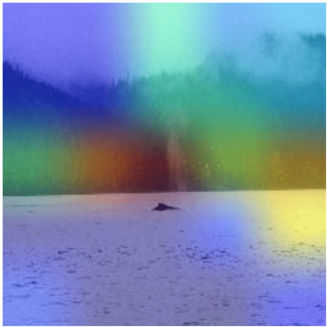
Understanding why a Neural Network predicts a certain way is crucial for conservation work, where biologists may verify that the algorithm focuses on biologically meaningful visual cues rather than the background. We therefore created Gradient-weighted Class Activation Maps (Grad-CAM) for a few images.

Code Excerpt

To create effective heatmaps, a two-step process is used. First, the code generates an activation map for a specific image. Then, it overlays the activation map on the original image. The TensorFlow code that implements this is below:

The resulting images, shown below, highlight the pixels that most affected the prediction for a given individual. This provides conservationists with visual confirmation that the CNN is focusing on meaningful regions of images.

4.3 Model Robustness to Image Quality Degradation

To quantitatively assess the model’s performance in real-world imaging conditions, we systematically evaluated its performance under controlled image quality degradations. A subset of 500 validation images provided by the Happywhale competition was processed with varying levels of Gaussian blur ( = 0.5, 1.0, 2.0 ) and brightness reduction (reduction of 70%, 60%, 50%). This simulates real-world variances commonly seen in images.

Results showed a reasonable degradation in performance:

• A moderate blur ( = 1.0) reduced the MAP@5 from 0.86 to 0.76.
• A severe blur ( = 2.0) on validation images dropped the MAP@5 from 0.86 to 0.69.
• Low-light conditions (60% of original brightness) reduced the MAP@5 from 0.86 to 0.80.
• A moderate blur ( = 1.0) and low-light conditions (60% of original brightness) reduced the MAP@5 to 0.7.

This model demonstrates strong resilience to brightness variations, likely due to grayscale conversion during training. These findings confirm that our model training strategies and image augmentations enhance the robustness of our model to real-world image variations.

4.4 Misclassification Analysis

Most mistakes made by the EfficientNetB5 & ArcFace model resulted when two separate species were visually similar. For example, the Bottlenose and Spinner dolphins had large amounts of training data; however, they were misclassified due to visual similarity and image quality.

Errors in classification also commonly occur when the number of images of a certain species is low. For example, the Fraser’s and Pygmy Killer Whale had a low accuracy relative to other classes, despite measures taken to reduce the effects of limited training data availability. In addition, images that demonstrate heavy motion blur, back lighting, or a lack of scars result in errors in classification. Below is a Grad-CAM heatmap of a misclassified image, in which the model focuses on features of the image that are irrelevant to classification:

Metric	Mean ± SD	95% CI	Fold Range
MAP@5	88.6% ± 0.4	[88.3%, 88.9%]	88.1%-89.2%

4.5 Cross-Validation Performance and Reliability

Performing cross-validation analysis revealed consistent model performance across several evaluation metrics. The narrow confidence intervals ( 1.0% width for accuracy and MAP@5) suggest robust generalizability for the model.

By measuring performance variability using standard deviation and confidence interval computations, and demonstrating metric stability across multiple data partitions, our findings meet the requirement for statistical validation.

4.6 Comparison with Other Happywhale Leaderboard Models

The Kaggle Happywhale – Whale & Dolphin Identification challenge attracted a total of 1,588 teams, and the Private Leaderboard, which is comprised of about 76% of the test data, is used to create the final standings for the competition. The “Preferred Dolphin” team attained the highest competition-wide Private Score of 0.876. The model blend attained a Private Score of 0.831. This model is ranked 76, placing it higher than about 95.12% of competitors¹¹.

5. Discussion

The performance of the different models tested in this work provides a series of lessons learned about both the challenges and solutions proposed for the individual identification of whales and dolphins. Analyzing the architecture, optimization strategies, and data augmentation techniques employed by various models enables us to identify the factors that contribute most to their relative success.

5.1 Basic CNN Model

The Basic CNN Model was implemented using a barebones Convolutional Neural Network (CNN) that served as a baseline model to achieve a score of 0.10. We can attribute its limited predictive capabilities to several shortcomings apparent in its design and training. Firstly, the architecture of the model required more depth and complexity to increase the model’s discriminative capabilities. The model consisted of only four convolutional layers and a limited number of image adjustments, both of which contributed to low accuracy. This model typically struggled to capture the intricate patterns present in the marine mammals in this dataset, such as unique pigmentation, scars, and fin shapes that may be used to distinguish among individuals. This is critical for the Happywhale datset. Additionally, the input images were trimmed, resulting in the loss of fine-grained details necessary for classification.

Additionally, the data augmentation techniques utilized in the Basic CNN Model—such as rotation, width/height shifts, and zoom—fell short in replicating the varied viewing angles, lighting conditions, and occlusions typical of real-world images. The implementation of a dropout layer at a 50% rate to prevent overfitting might have unintentionally restricted the model’s capacity to capture subtle features. Furthermore, sparse categorical cross-entropy was adopted as the loss function, yet without incorporating more sophisticated methods, such as margin-based loss, which would have constrained the model’s effectiveness in differentiating between visually similar individuals more effectively.

5.2 ResNet and ArcMargin Model

The ResNet and ArcMargin Model introduced significant improvements in accuracy by utilizing a ResNet-based architecture and incorporating the ArcMargin loss function, resulting in a notable increase in accuracy to 0.48. The ResNet backbone for this model enabled the model to recognize more nuanced patterns in images compared to the simple CNN. The ResNet and ArcMargin models also mitigated the vanishing gradient problem, reducing the likelihood of training rates stalling or stopping.

The use of the ArcMargin loss function increased the discriminative power of the models by adding an angular margin to the classification boundary between image labels. This resulted in increased discriminative capabilities for the model and a higher score using the MAP@5 metric.

However, the model’s performance plateaued due to certain restrictions on the training strategy and data. In this model, the ArcMargin loss function improved the separation between classes. However, it was not an optimal solution for every class in the Happywhale dataset, which contained an imbalance across the number of species of marine mammals. Additionally, the data processing techniques in this model were minimal, resulting in the model’s inability to recognize fine details present in this dataset’s images.

5.3 EfficientNetB5 and ArcFace Model

The EfficientNetB5 and ArcFace Model demonstrated a significant performance leap compared to previous models, achieving a MAP@5 score of 0.86. The ArcFace function enhanced distinctions between marine mammal classes by introducing angular boundaries, allowing the model to accommodate slight variations in individual appearance more effectively. This is crucial for Happywhale, where images of the same animal can vary due to lighting, pose, color, and environmental conditions, while differences between classes can be subtle¹².

The EfficientNetB5 backbone’s compound scaling strategy balanced depth, width, and resolution in the CNN. Training at 380×380 resolution enabled the model to capture intricate image details. Improved data augmentation techniques, including grayscale transformations, color adjustments, and random cropping, reduced the likelihood of overfitting. K-fold cross-validation ensured good generalization to unseen data¹³.

5.4 Model Performance Gap

The 38-point jump in MAP@5 accuracy is the joint result of four architectural and training changes introduced in the EfficientNetB5 and ArcFace Model compared to ResNet and ArcMargin Model. The key factors contributing to this performance are listed below:

1. Backbone capacity and resolution

ResNet-50 processes 224 x 224 px inputs and relies on uniform down-sampling. Much granular detail contained in images of the Happywhale dataset is lost. However, EfficientNet-B5 paired with “compound scaling” retains fine scar and pigmentation details. Constraining the EfficientNet-B5 to 224 x 224 px reduces the accuracy due to a loss of key features contained in images.

2. Loss Formulation

ArcMargin uses a fixed angular margin, and classes with a few images fail to cross this set threshold. ArcFace instead samples the margin from each mini-batch, creating a boundary that adapts to variations within a class. Switching ResNet to ArcFace is a second cause of the performance jump between ResNet + ArcMargin and EffNetB5 + ArcFace.

3. Multi-crop augmentation

The ResNet baseline employed only flips and color changes, whereas the EfficientNet-B5 model utilizes full-body, YOLOv5, Detic, or Vision Transformer. This exposes the model to images that only display certain parts of a marine mammal, as well as the full body of the animal.

4. Imbalance Mitigation

Happywhale is heavily skewed (9,664 images for bottlenose_dolphin vs. 14 for Fraser’s dolphin). The EfficientNetB5/ArcFace model mitigated the effects of this by utilizing an ArcFace loss function, minority oversampling, and other methods.

5.5 Model Blend (Ensemble)

Our final submission is an ensemble of 30 model checkpoints, each chosen for its unique strengths. Twenty-five are “generalist’’ models trained on the full dataset with different resolutions, crop pipelines, and augmentation recipes. The other five are specialist models focused on beluga-only, back-fin, or full-body crops that do not make the systematic errors made by the generalists.

At inference time, each model outputs its five most likely individual IDs. These ranked lists are combined with the weighting scheme and frequency penalty detailed in the Weight optimization paragraph of the same section. Because all coefficients were tuned only on out-of-fold (OOF) data, the blend generalizes well, improving the best single checkpoint (MAP@5 = 0.854) to 0.88 MAP@5 on Kaggle’s public leaderboard.

This concise overview avoids repeating the optimization mechanics while preserving the high-level rationale, composition, and performance of the ensemble.

5.6 Model and Dataset Limitations

While the Happywhale dataset is one of the largest publicly available collections of various marine mammals, it has several limitations that affect the model’s performance and real-world applicability.

The dataset shows significant geographic bias, with the majority of reported sightings concentrated in the central and eastern North Pacific regions, such as Hawai’i and Alaska. In contrast, areas in the Western Pacific are significantly under-sampled due to reduced populations in those regions. This disparity is even more pronounced in remote areas critical for whale populations, such as the Revillagigedo and Aleutian Islands. As a result, models trained using the Happywhale dataset will likely perform poorly due to the limited training data available on marine mammals in those areas¹⁴.

Temporal bias is another important consideration. The Happywhale dataset reflects significant fluctuations in sampling intensity over time, with peak image reporting during the 2004-2006 SPLASH project. Image reporting lessened during the COVID-19 pandemic, despite thriving marine mammal populations during this time¹⁵.

5.7 Key Model Insights

1. Loss Functions: Transitioning from basic cross-entropy loss functions to more advanced ArcMargin and ArcFace loss functions had a positive impact on the models’ ability to classify marine mammals. While cross-entropy loss functions are effective for most tasks, they typically focus solely on minimizing the error percentage rather than enforcing the separation of different classes in the parameter space. However, the ArcMargin loss function introduced an angular margin to separate classes, forcing the model to place the predictions farther apart. This enhances the model’s ability to distinguish between visually similar species while maintaining its capacity to classify images effectively. Finally, the ArcFace Loss function builds on ArcMargin by adding an angular separator between categories. This allowed the model to be more robust to slight variations in images caused by things such as lighting or camera angles.
2. Model Architectures: The use of model architectures was also critical to the success of more advanced models. The use of the EfficientNetB5 model architecture allowed the model to outperform the basic CNN architecture. This is attributed to this backbone’s ability to effectively scale across various levels of depth, width, and resolution. Selecting architectures that strike a balance between computational efficiency and representational power is important for this machine learning task.
3. Data Augmentation: Using data augmentation techniques enhances the robustness of the models through grayscale transformations and color adjustments. This highlights the importance of data augmentation strategies in simulating real-world image variations and enabling the model to generalize effectively.
4. Ensembles: The ensemble approach to this Machine Learning challenge showed how combining multiple perspectives on the same data produces significantly better results. Model four effectively leveraged the various strengths in snapshots, resulting in improved performance in the dataset.
5. Class Imbalance Limitations: Although our approach to handling imbalances proved effective, the extreme imbalance still remains a challenge. Traditional rebalancing techniques were deemed inappropriate for this task due to the potential loss of critical natural ecological patterns in images .
6. Handling Imbalanced Data: The Happywhale dataset has an uneven distribution of images, with an imbalance in the number of training samples for certain individuals. However, our models resolved this issue by utilizing margin loss and cross-validation, which helped the model generalize and become more robust to unseen data.

5.8 Practical Applications

While the technical performance of our machine learning model shows some promise, successfully making an impact on conservation efforts requires integration into existing workflows. This subsection examines the practicality of this CNN-based approach for identifying marine mammals in the real world. Integration with Photo Identification Databases: Citizen science portals and research archives, such as Flukebook, already contain lists of records for thousands of animal images. To effectively utilize the CNN, it can be integrated into an API that receives an uploaded image, returns the top identity labels for the image, and stores them alongside labels assigned manually by humans. This lightweight integration minimally interferes with a conservationist’s workflow while providing benefits¹⁶.

Public Engagement and Education: Embedding the model in a mobile app that allows users to upload images to the cloud enables whale watchers to receive instant feedback on animals they have photographed. This follows the success of bird identification apps, which have increased public participation and raised awareness about ornithology¹⁷. In addition, images uploaded to the mobile app may be used to improve models further, creating a positive feedback loop of model improvement and public participation.

5.9 Comparison with Prior Work

Existing marine mammal photo-identification systems consistently report strong performance on specific tasks. Some examples include:

• finFindR, created by J. Thompson et al. in 2021 achieved an 88% rank-1 match rate and 97% rank-50 success on common bottlenose dolphins when evaluated¹⁸.
• FIN-PRINT, created by C. Bergler et al. in 2021 scored 92.5% top-1 accuracy and 97.2% top-3 accuracy on 100 frequently photographed killer-whale individuals¹⁹

Our ensemble achieves 0.88 MAP@5 (public) and 0.831 MAP@5 (private), ranking 70 out of 1,588 teams. Although the evaluation metrics performed are different, the results show that our multi-species classification model has lower accuracy but stronger generalization across the 30 species presented in the Happywhale dataset.

6. Conclusion

This study applies advanced deep learning methodologies to address the challenge of identifying marine mammals using the Happywhale dataset. The models leveraged modern convolutional architectures, loss functions, and data augmentation strategies. This research efficiently addresses the challenge of classifying fine-grained image data to advance ecological research. This study showcased models that evolved from a baseline CNN model with limited classification capabilities to high-performing models that incorporate advanced backbones and loss functions, effectively making predictions. This study also acknowledges and addresses the significant class imbalance present in the dataset, showcasing a non-traditional strategy to mitigate its effects.

The iterative approach of progressing through four separate models demonstrates that refining components, ranging from network depth to augmentation methods, can lead to breakthroughs in the performance of the machine learning model. Specifically, the KNN algorithm proved to be critical in categorizing unseen images while maintaining a clear, defined boundary between marine mammal species. Using all the techniques described in this study, an identification system has been created to assist environmentalists in tracking marine mammal populations without relying on labor-intensive manual matching.

Beyond its immediate application, this research contributes to the field of wildlife conservation by providing an efficient and scalable method for tracking species. The model’s ability to identify marine mammals is crucial for monitoring populations and protecting marine ecosystems.

From a broader perspective, the findings in this study show the practicality and importance of implementing deep learning solutions to monitor wildlife and draw inferences on carrying capacity, food webs, and other related aspects. The use of machine learning also provides an instant mechanism to support ecological studies and inform conservation programs. This research demonstrates how machine learning helps bridge the gap between technology and environmental science, proving to be a vital tool for preserving marine ecosystems for future generations. The approaches utilized and the lessons learned during this study pave the way for broader adoption of Machine Learning in ecological research.

7. References

1. K. N. Shivaprakash, N. Swami, S. Mysorekar, R. Arora, A. Gangadharan, K. Vohra, M. Jadeyegowda, J. M. Kiesecker. Potential for artificial intelligence (AI) and machine learning (ML) applications in biodiversity conservation, managing forests, and related services in India. Sustainability. 14, 7154 (2022). [↩]
2. T. Cheeseman, K. Southerland, W. Reade, A. Howard. Happywhale – whale and dolphin identification: overview. https://www.kaggle.com/competitions/happy-whale-and-dolphin/overview (2022). [↩]
3. NOAA Fisheries. Marine mammal photo-identification research in the southeast. https://www.fisheries.noaa.gov/southeast/endangered-species-conservation/marine-mammal-photo-identification-research-southeast (2024). [↩]
4. M. Tan, Q. V. Le. EfficientNet: rethinking model scaling for convolutional neural networks. https://arxiv.org/pdf/1905.11946 (2020). [↩]
5. J. Deng, J. Guo, J. Yang, N. Xue, I. Kotsia, S. Zafeiriou. ArcFace: additive angular margin loss for deep face recognition. https://arxiv.org/abs/1801.07698 (2018). [↩]
6. T. Cheeseman, K. Southerland, W. Reade, A. Howard. Happywhale – whale and dolphin identification: dataset description. https://www.kaggle.com/competitions/happy-whale-and-dolphin/data (2022). [↩]
7. Google Developers. Datasets: imbalanced datasets. https://developers.google.com/machine-learning/crash-course/overfitting/imbalanced-datasets (2025). [↩]
8. Kaggle. Tensor processing units (TPUs). https://www.kaggle.com/docs/tpu (n.d.). [↩]
9. 9. L. E. Peterson. K-nearest neighbor. http://var.scholarpedia.org/article/K-nearest_neighbor (2009). [↩]
10. J. Brownlee. Blending ensemble machine learning with Python. https://machinelearningmastery.com/blending-ensemble-machine-learning-with-python/ (2021). [↩]
11. T. Cheeseman, K. Southerland, W. Reade, A. Howard. Happywhale – whale and dolphin identification: leaderboard. https://www.kaggle.com/competitions/happy-whale-and-dolphin/leaderboard (2022). [↩]
12. J. Deng, J. Guo, N. Xue, S. Zafeiriou. ArcFace: additive angular margin loss for deep face recognition. Proceedings of the IEEE/CVF Conference on Computer Vision and Pattern Recognition. 4690–4699 (2019). [↩]
13. C. Shorten, T. M. Khoshgoftaar. A survey on image data augmentation for deep learning. Journal of Big Data. 6, 60 (2019). [↩]
14. P. T. Patton, T. Cheeseman, K. Abe, T. Yamaguchi, W. Reade, K. Southerland, A. Howard, E. M. Oleson, J. B. Allen, E. Ashe, A. Athayde, R. W. Baird, C. Basran, E. Cabrera, J. Calambokidis, J. Cardoso, E. L. Carroll, A. Cesario, B. J. Cheney, E. Corsi, J. Currie, J. W. Durban, E. A. Falcone, H. Fearnbach, K. Flynn, T. Franklin, W. Franklin, B. Galletti Vernazzani, T. Genov, M. Hill, D. R. Johnston, E. L. Keene, S. D. Mahaffy, T. L. McGuire, L. McPherson, C. Meyer, R. Michaud, A. Miliou, D. N. Orbach, H. C. Pearson, M. H. Rasmussen, W. J. Rayment, C. Rinaldi, R. Rinaldi, S. Siciliano, S. Stack, B. Tintoré, L. G. Torres, J. R. Towers, C. Trotter, R. Tyson Moore, C. R. Weir, R. Wellard, R. Wells, K. M. Yano, J. R. Zaeschmar, L. Bejder. A deep learning approach to photo-identification demonstrates high performance on two dozen cetacean species. Methods in Ecology and Evolution. 14, 2611–2625 (2023). [↩]
15. T. Cheeseman, K. Southerland, J. M. Acebes, K. Audley, J. Barlow, L. Bejder, C. Birdsall, A. L. Bradford, J. K. Byington, J. Calambokidis, R. Cartwright, J. Cedarleaf, A. J. García Chavez, J. J. Currie, J. De Weerdt, N. Doe, T. Doniol-Valcroze, K. Dracott, O. Filatova, R. Finn, K. Flynn, J. K. B. Ford, A. Frisch-Jordán, C. M. Gabriele, B. Goodwin, C. Hayslip, J. Hildering, M. C. Hill, J. K. Jacobsen, M. E. Jiménez-López, M. Jones, N. Kobayashi, E. Lyman, M. Malleson, E. Mamaev, P. Martínez Loustalot, A. Masterman, C. Matkin, C. J. McMillan, J. E. Moore, J. R. Moran, J. L. Neilson, H. Newell, H. Okabe, M. Olio, A. A. Pack, D. M. Palacios, H. C. Pearson, E. Quintana-Rizzo, R. F. Ramírez Barragán, N. Ransome, H. Rosales-Nanduca, F. Sharpe, T. Shaw, S. H. Stack, I. Staniland, J. Straley, A. Szabo, S. Teerlink, O. Titova, J. Urban, M. van Aswegen, M. Vinicius de Morais, O. von Ziegesar, B. Witteveen, J. Wray, K. M. Yano, D. Zweifelhofer, P. Clapham. A collaborative and near-comprehensive North Pacific humpback whale photo-ID dataset. Scientific Reports. 13, 10237 (2023). [↩]
16. Flukebook. A.I. for cetacean research. https://www.flukebook.org/ (n.d.). [↩]
17. P. Leonard. AI-powered BirdNET app makes citizen science easier. https://news.cornell.edu/stories/2022/06/ai-powered-birdnet-app-makes-citizen-science-easier (2022). [↩]
18. J. W. Thompson, V. H. Zero, L. H. Schwacke, T. R. Speakman, B. M. Quigley, J. S. Morey, T. L. McDonald. finFindR: automated recognition and identification of marine mammal dorsal fins using residual convolutional neural networks. Marine Mammal Science. 38, 139–150 (2021). [↩]
19. C. Bergler, A. Gebhard, J. R. Towers, L. Butyrev, G. J. Sutton, T. J. H. Shaw, A. Maier, E. Nöth. FIN-PRINT a fully-automated multi-stage deep-learning-based framework for the individual recognition of killer whales. Scientific Reports. 11, 23480 (2021). [↩]