Classification of W-R Stars using K-means and KNN Machine Learning Models

Abstract

Wolf-Rayet (W-R) stars, known for their high mass loss rates and extreme stellar winds, are irregular stars beyond O-type stars in the Hertzsprung-Russell (H-R) diagram. These evolved, massive stars shed their outer hydrogen layer to form planetary nebulae and enrich the interstellar medium with heavier elements. W-R stars can be subtyped as WN (nitrogen-rich), WC (carbon-rich), or WO (oxygen-rich) based on spectral features. In this study, we hypothesized that B-V color index, stellar wind velocity, and absolute visual magnitude are all equally important factors for sub-classifying WN and WC stars. We utilized two machine-learning models, K Nearest Neighbors (KNN) and K-means, to classify W-R stars based on these 3 parameters. Additionally, we also predicted that the KNN model will outperform the K-means in classification. We used a dataset of ~200 W-R stars from the VizieR VII catalog and applied K-Nearest Neighbors (KNN) and K-means clustering for classification. The KNN model achieved 75.76% accuracy, outperforming K-means at 60.29%. Dummy classifiers achieved ≤55.38%, contextualizing KNN’s superior performance. Confusion matrices, F1-scores, precision, and recall provided deeper insights, revealing KNN’s strength in detecting WC stars, while K-means showed balanced performance. Permutation importance and ablation testing confirmed stellar wind velocity as the most critical feature. A McNemar’s test validated KNN’s statistically significant superiority over K-means. Despite the limited dataset, this study presents a foundational framework for interpretable, data-efficient machine learning in stellar classification.

Introduction

Irregular stars are stars outside the normal range of classification on the Hertzsprung-Russell diagram. Some examples of irregular stars are Wolf-Rayets, Blue Stragglers, and Red Clump stars. These stars typically have unique properties compared to average stars, such as broader or narrower emission lines or higher masses and temperatures. These stars have special classifications, which are WR, L, T, Y, S, and C. Wolf-Rayets are one of these irregular stars, usually well into their later stages of evolution, but are believed to start as an O-type star. They are characterized by strong solar winds, extreme mass loss, and high temperatures. Typical Wolf-Rayet stars have lost most of their outer hydrogen and have moved on to fusing helium and other heavier elements in their core. They are usually around 40+ solar masses and have a temperature range of 25,000 K – 50,000 K. Helium, nitrogen, and carbon emission lines often dominate Wolf-Rayet stars, allowing them to be separated into three categories based on the spectra: WN, WC, and WO, where WN is nitrogen-dominated, WC is carbon-dominated, and WO has a C/O ratio of less than 1. They would end their life as a Type Ib or Type Ic supernova and are relatively rare, with only around 220 observed in the Milky Way.

Wolf-Rayet stars were first discovered by 2 French astronomers, Charles Wolf and Georges Rayet, in 1867. They first noticed these types of stars when observing the Cygnus constellation. Wolf and Rayet then observed that three stars in the constellation gave broad emission lines that differed from the rest of the otherwise continuous spectrum¹. Stars typically have absorption lines in their spectra due to light from the stars’ interior passing through relatively cooler gas on the surface, which absorbs photons of certain wavelengths that indicates the elemental composition. Since Wolf and Rayet observed emission lines instead, they figured they were dealing with an unusual type of star. Astronomers originally did not understand why emission lines were shown on the spectra, but it was later found that these emission lines were caused by helium, which was discovered in 1868². Astronomers noticed that the spectra of these newly found Wolf-Rayet stars were similar to that of nebulae, leading them to believe that these stars were the centers of planetary nebulae³. The abnormal width of the emission bands on the Wolf-Rayet star spectra was discovered to be caused by Doppler broadening (the broadening of spectra lines due to the Doppler effect caused by varying velocities of gas) later in 1929⁴. This led to the hypothesis that Wolf-Rayets are constantly spewing gas into space, creating a nebula.

This leads us to our driving questions: Could W-R stars be classified into either WN or WC types using a machine learning model with only the B-V color-magnitude, visual magnitude, and stellar wind speeds as the parameters, and which model between the KNN and K-means would be the most accurate at classifying these stars based on the three parameters? For this study, we hypothesized that the KNN model would be more accurate than the K-means model when classifying Wolf-Rayets between WN and WC types, and that all three parameters are essential for the classification process. We found that the KNN model was more accurate than the K-means model, and the stellar wind velocity was the most influential parameter of the three, followed by B-V color index and absolute visual magnitude.

This study paper is scientifically important in many ways. Firstly, it significantly adds knowledge to the current understanding of these Wolf-Rayets, as only about 200 are observed in our Milky Way galaxy. Studying these stars can give us insight into their physical and chemical properties and how they affect nearby objects. Secondly, an improved understanding of these stars can help astronomers with their current models and how they are affected by Wolf-Rayets and their properties. Lastly, studying the chemical composition can give us a better understanding of how a Wolf-Rayet’s properties are altered, such as their luminosity, temperature, etc.

Results

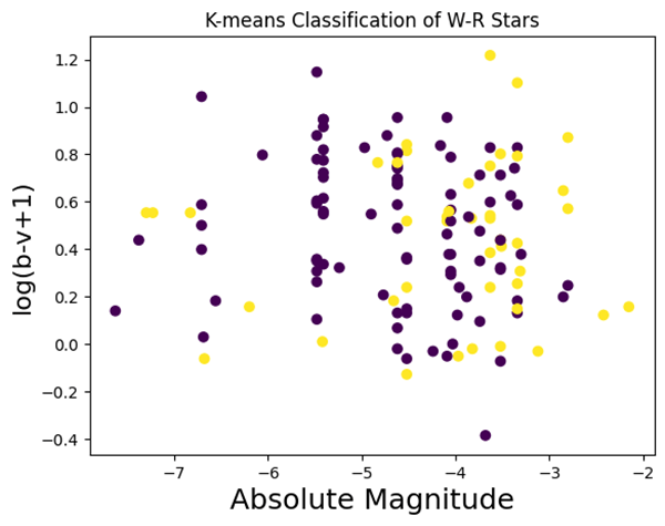
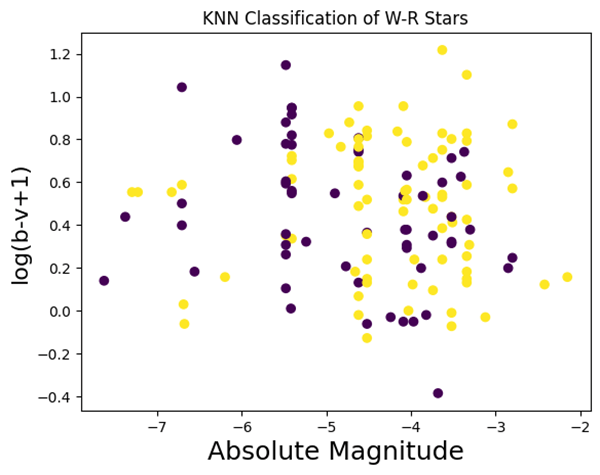
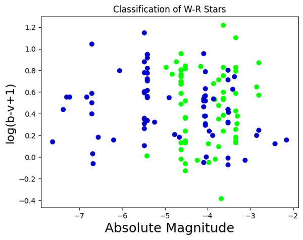
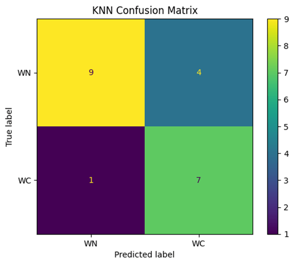
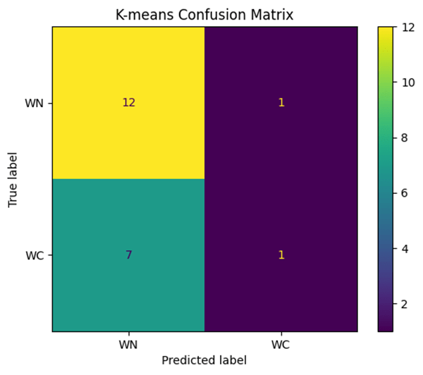
After training and testing both models, we found that the K-means model had an accuracy of 60.29% (Fig. 1) compared to the actual classification given by the catalog (Fig. 3). The KNN model performed better, with an accuracy of 75.76% (Fig. 2).

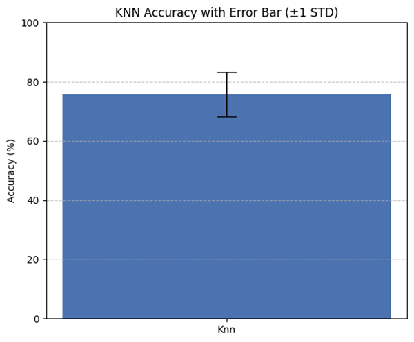
Our KNN model accuracy, with a standard deviation of 7.5%, was found by averaging the results of 100 test runs.We have added an error bar of ±1 standard deviations in Figure 4 to visualize the variance.

To support the reported 75.76% KNN accuracy, we used several dummy classifiers as performance baselines. The most frequent class classifier scored 55.38% accuracy, the stratified classifier scored 51.14%, the uniform classifier scored 49.14%, and the constant classifier (predicting the dominant class) also scored 55.38%. These baseline classifiers highlight the effectiveness of the KNN model in capturing meaningful patterns in the data. This further aids the KNN model’s ability to perform better than naive classification strategies.

As part of a formal feature importance analysis, we performed permutation importance to determine the impact of the three parameters on the KNN model. This method randomly permutes each feature to assess its effect on model accuracy. Wind velocity had a positive importance score of 0.1524, whereas both the B-V color index and absolute visual magnitude yielded slightly negative scores of -0.0190 and -0.0286, respectively. This indicated that wind velocity is the most influential parameter for classification, while B-V color index and absolute visual magnitude had marginal effects on accuracy. Given KNN’s sensitivity to noise and redundancy, this feature importance analysis implies that the B-V color index and absolute visual magnitude slightly introduced some overlap in feature space. These results contrast slightly with our ablation testing results, which helps offer nuanced insights into the effects of the parameters. Overall, these findings reveal that the wind velocity had the most impact among the three parameters, although the combination of all three features may still help the model detect more complex patterns. Furthermore, to evaluate the performance of each parameter and its effects on classification performance, we conducted ablation testing on the KNN model. When all three parameters were used, the accuracy of the model was 75.76%. When we removed the B-V color index, the accuracy of the model slightly increased to 77.62%, suggesting that this parameter played a minimal role and had a small, negative impact on classification. Furthermore, when the stellar wind speed was removed, the accuracy went up to 87.29%, indicating that the parameter may hurt the classification accuracy. On the other hand, when the absolute visual magnitude was removed, the accuracy dropped to 73.90%, implying the important, positive nature of the parameter on accuracy. With these results, our earlier assumption that all three parameters play an important role is challenged and provides insights that absolute visual magnitude has a strong positive impact on the model, the B-V color index has a less, or sometimes negative, impact on classification performance, and stellar wind speed has a strong negative impact on the model’s accuracy. Thus, we acknowledge that all three parameters do not have an equal impact in the classification performance, contrary to our hypothesis.

We also assessed the K-Means model using accuracy, which is not ideal for clustering methods. Accuracy assumes a direct correspondence between clusters and known classes, which is not inherently true in unsupervised learning. To provide a more appropriate evaluation, we compared the K-Means cluster assignments to the true labels using Normalized Mutual Information (NMI) and Adjusted Rand Index (ARI). These metrics measure the similarity between clustering results and ground truth without assuming label alignment. The K-Means model achieved an ARI of 0.0666 and an NMI of 0.1411, indicating only modest agreement with the actual WN/WC classifications. This suggests that, without domain-specific feature engineering, unsupervised algorithms like K-Means have limited ability to recover astrophysical subtypes. Furthermore, the resulting clusters may instead reflect intrinsic data groupings that do not align with established astrophysical categories such as WN and WC stars.

We ran a McNemar’s test between the classification outputs of the KNN and K-means models to determine if the difference in the models’ accuracies were statistically significant. Since the two models in our case were analyzing the same dataset, we chose to conduct a McNemar’s test with the nominal paired data. Our contingency table showed that KNN correctly classified 4 instances that K-means misclassified, while K-means correctly classified 2 instances that KNN misclassified:

	KNN Correct	KNN Incorrect
K-means Correct	4	12
K-means Incorrect	2	3

McNemar’s test yielded a p-value of 0.0162, and the test statistic is 5.7857 with α = 0.05. Our p-value indicates that the difference in the accuracy between KNN and K-means is statistically significant, therefore we have evidence to reject the null hypothesis. We conclude that the KNN model significantly outperforms the K-means model in classification of Wolf-Rayet subtypes.

We also included other performance metrics beyond accuracy, which can be distorted by class imbalance. We calculated precision, recall, and F1-scores for the KNN and K-means models. KNN showed a higher precision of 0.86 for WN stars, but a much lower recall of 0.46. This suggests that while KNN was precise in predicting WN stars, it missed many actual WN stars. On the other hand, the model achieved a high recall of 0.88 but a lower precision of 0.50 for WC stars, highlighting that it correctly identified most WC stars but with some false positives. The macro-averaged F1-score for KNN was 0.62. K-means, conversely, showed a much more balanced performance across both classes, with a precision and recall of 0.73 and 0.85 for WN and 0.67 and 0.50 for WC, respectively.

Model	Class	Precision	Recall	F1-Score	Support
KNN:	WN	0.86	0.46	0.60	13
	WC	0.50	0.88	0.64	8
	Macro Avg	0.68	0.67	0.62	21
	Weighted Avg	0.72	0.62	0.61	21
K-Means:	WN	0.73	0.85	0.79	13
	WC	0.67	0.50	0.57	8
	Macro Avg	0.70	0.67	0.68	21
	Weighted Avg	0.71	0.71	0.70	21

Using a confusion matrix, we found that our KNN model classifies WC-type stars to a higher degree of accuracy compared to WN. This also revealed that the model leans toward WC-type stars and struggles with WN when classifying (Fig. 6). K-Means had a substantially worse accuracy, as it classified nearly all of the stars as WN (Fig. 7).

These machine learning models allow us to test multiple parameters and find which data points are the most relevant in classifying W-R stars into their subcategories. Overall, our findings from different tests and analyses highlight that the KNN model outperforms the K-means in the sub-classification of W-R stars.

Materials and Methods

K-nearest neighbor is an algorithm that uses the proximity between data points to classify the points. The “k” in KNN defines the number of nearby points that the algorithm considers when making a classification. The algorithm identifies the most common neighbor and classifies the new data point as such. On the other hand, K-means is a model that separates a data set into several clusters. The algorithm selects several central points as “centroids” and utilizes them to form clusters with nearby data points. The centroids are updated based on the mean of the data values in the cluster and form new clusters based on the new location. This process repeats until the position of the centroids stops moving. This results in separate data clusters of similar data points, classifying the data into “k” different groups. The parameters we focused on to separate the star types were the B-V color index (a comparison between the star’s blue (B) light and combined visible (V) light), stellar wind velocities (speeds of materials ejected from the stars) in km/s, and absolute visual magnitude (the star’s true luminosity regardless of distance). We sourced our data from the VizieR catalog, a public astronomical catalog created by the European Space Agency that contains data on many stellar objects. Out of the 3 main types of W-R stars (WN, WC, WO), we only differentiated between WN and WC types due to the limited data available in datasets on WO-type W-R stars.

To find data for our models, we searched the VizieR database for tables with data on Wolf-Rayet stars. The result we received from the initial search was 3 different catalogs: 7th Catalog of Galactic Wolf-Rayet stars (van der Hucht, 2001) indexed as III/215, Physical parameters of Wolf-Rayet galaxies (Brinchmann+, 2008) indexed J/A+A/485/657, and Sixth Catalogue of Galactic Wolf-Rayet Stars (van der Hucht+ 1981) indexed as III/85 which later became obsolete due to III/215. We also ruled out catalog J/A+A/485/657 as it focused on the physical properties of Wolf-Rayet galaxies, not solely the stars. That left us with catalog III/215, which has 226 rows of data on Wolf-Rayet stars. Catalog III/215 had 6 table labels: Table 13 titled “Locations of galactic WR stars”, Table 14 titled “Environment of galactic WR stars”, Table 15 titled “Parameters of galactic WR stars”, and Table 28 titled “Photometric distances of galactic WR stars”, and lastly 2 reference tables, which we didn’t use since they held no data. From the remaining 4 tables (13, 14, 15, and 28), we sorted through the data and chose our three parameters. We also added some extra data like Right Ascension and Declination for each WR star, the identification number within the tables (specifically from within Table 13), and the star’s WR classification (WC, WN, or WO types). After choosing the data, we combined several parameters into a table and created a .csv file. Due to the limited data in the VizieR catalog, as mentioned before, we were pushed to exclude many other important astrophysical parameters that have been used for stellar classification, like metallicity, luminosity class, and spectral line diagnostics. Particularly, many of these parameters either had incomplete data or were not included in the database which hindered our ability to develop accurate models that supported a wider range of classification parameters. To ensure uniformity and accuracy in our results, we chose to stick with the three well-documented parameters that were available in our dataset. We also made a chart summarizing key statistics of our 3 parameters: the mean value, count, minimum and maximum values, and standard deviation.

	Absolute Magnitude	B-V	Wind Speed (Km/s)
Count	136.00	194.00	141.00
Mean	-4.48	0.91	1721.70
Std	1.11	1.57	714.20
Min	-7.63	-0.32	90.00
Max	-2.150	21.10	5000.00

We began with 226 WR stars before data cleaning. We cleaned our dataset by removing stars that had any missing information, which left us with 136 stars. From the remaining stars, we utilized 115 for training and 21 for our testing, following an 85/15 split. This informs us of the small size of the dataset, meaning that the models are therefore more prone to errors and restricted generalization to unseen Wolf-Rayet stars. While a larger dataset may result in more accurate predictions, the catalog we used was limited in its data, and our current models still had acceptable accuracies and results. Moreover, the majority of effects like the reduction in strength of conclusions made from the accuracy are weakened, which draws upon the decreased statistical power to separate between the differences in performance between the models.

A challenge in this study was the class imbalance between WN and WC-type Wolf-Rayet stars. Of the 136 usable stars after cleaning, 75 were WN and 61 were WC. To reduce the risk of model bias toward the majority class, we applied stratified random undersampling to the WN class in the training set, selecting a subset equal in size to the WC sample. This approach ensured balanced class representation during training for both our KNN and K-means models, allowing for fairer classification between the subclasses and minimizing skew in the resulting predictions. Normalization of data was also ensured to reduce any parameter from dominantly affecting the final classification that can arise from disparities in units. Regardless, the chosen parameters were plentiful in leading a data-driven, well-designed classification of W-R stars into WN and WC types. We then fed the cleaned-up data to the KNN and K-Means machine-learning models in Python using Visual Studio Code and Jupyter Notebook.

Data was split as 85% training data and 15% testing data. The accuracy scores were averaged from 100 runs to lower variance and generate a standard deviation for our model accuracies. In order to choose our k value, we ran a loop from 1 to 25 neighbors in each of the 100 runs to select and use the optimal value that resulted in the best accuracy. Additionally we used the standard Euclidean distance as the similarity metric for KNN. On the other hand, the K-means model was set up using 2 clusters for the WN and WC-types, rather than 3, as there was a lack of data for WO-type stars.

Discussion

To solidify our overall findings, we decided to find some peer-reviewed academic sources to compare our results with and to guide us toward using a better model. We used the study Machine-Learning Approaches to Select Wolf-Rayet Candidates: Proceedings of the International Astronomical Union, which dives into classifying normal stars and Wolf-Rayets using the KNN model⁵. We used this study that took in the potential Wolf-Rayet candidates and implemented the KNN model to further classify Wolf-Rayet stars into their subcategories (WN or WC). This source provided us with the foundations we needed to begin our research and had a lot of accurate information on the classification between Wolf-Rayets and normal stars that we used for our study. Additionally, another study by Giuseppe Morello and colleagues⁶  dived into classifying W-R stars using the K-nearest neighbor (KNN) model we used for our classification. This paper primarily used infrared color selection as the main parameter of classification to distinguish between normal stars and W-R stars. It aimed to provide an efficient method of classification, an automated classifying tool, and statistical data geared towards the differentiation of a normal and W-R star. In our case, we decided that the KNN model would work better due to its higher efficiency and accuracy compared to the K-means model, and this paper provides more foundational support for our conclusion. Using KNN, both papers provided a more accurate classification of W-R stars, although our parameters vary. These papers help establish the support for our KNN model and guide us in providing accurate classifications.

Our primary focus on employing the K-Nearest Neighbors (KNN) and K-means clustering models was due to multiple reasons. They allow for the incorporation and usage of small to medium-sized datasets, which has been a major issue and limitation that we faced with our constrained Wolf-Rayet dataset. Furthermore, the two models are easy to interpret, have high conceptual simplicity, and have been given a lot of preference in the past in astrophysical research and classification. Finally, the KNN model, which has been used in past research to classify other irregular stars, including some Wolf-Rayet candidates, provides a solid footing for our research and methodology⁵’⁶. Although more advanced models exist,  like decision trees, SVMs, or ensemble classifiers, our research primarily focuses on the goal to establish a foundational classification structure that requires minute hyperparameter tuning and relatively easy interpretability. This allows us to focus on the influence of our three selected parameters rather than focusing on the complexity of model planning. Additionally, we assumed that input features do not contain any errors. In practical terms such values may prove observationally ambiguous due to weather conditions, instrument inaccuracy, and errors arising in the course of calibration. Also, some of the entries in the VizieR catalog lack confidence intervals or error bars which make it difficult to analyze. These measurement errors are likely to have an effect on the decision boundaries learnt by machine learning models and lead to lower precision and misclassifications.

In order to receive professional feedback, we presented our research to Dr. Karl Gebhardt, the chair of the Department of Astronomy at the University of Texas at Austin. He suggested that we switch from using the apparent magnitude that we initially thought of doing to the absolute magnitude available in the dataset. Furthermore, he also recommended that we try feeding the spectra of the stars into our machine-learning models directly, but we were unable to find spectra graphs for all the stars in the VizieR database. Lastly, he suggested we implement confusion matrices for our KNN and K-means to evaluate and solidify their performances.

After examining the instances, it was discovered that many of the WC-type stars that were incorrectly classified as WN shared traits that were different from those of typical WC distributions. For example, the wind velocities shown were lower than average for a typical WC star, and the B-V indices were much closer and occasionally overlapped with the WN class. Some of the models’ classifications were thrown off since both of our models relied on geometric distance or cluster density rather than astrophysical features. This relates to our focus to include more characteristics that can distinguish these differences in subsequent research to increase the precision of W-R star subclassification. While our current models provide baseline and relevant classifications, there are still some limitations regarding the uncertainty of overlap in parameters, particularly for WC stars. When we did a closer analysis on misclassified WC stars, we found that although class imbalance may have played a role in the misclassification, it was mainly the fact that the stars showed parameters values that were overlapping greatly with WN-type stars. For instance, the B-V indices for many of the WC stars were suspiciously blue to be counted for WC classification, and the wind velocities were relatively low (closer to that of the median of WN stars). When looking at these overlaps, we can infer that the WC stars form a cluster that is not distinct or separable. Furthermore, inherently, WC stars show a greater diversity of observed properties, making the process of classification through distance-based models like KNN or K-means complicated. Through this insight, we conclude that additional parameters such as metallicity are needed to improve model accuracy due to the overlap in wind speed and photometric data between WN and WC stars.

Lastly, we compared the performance of the KNN model with the K-means model, where the former is supervised and the latter is unsupervised. We acknowledge that this comparison, while providing insights into the potential of label-free classification, is not a direct benchmark for evaluating a supervised model like KNN. A more appropriate comparison in future work should incorporate additional supervised algorithms such as Random Forest, Support Vector Machines (SVM), and decision trees to enable more robust classification performance. Including these models would provide a stronger comparative foundation for KNN and allow future research to explore improvements in generalization, interpretability, and accuracy when classifying Wolf-Rayet stars.

Connclusion

In this study, we aimed to sub-classify Wolf-Rayet (W-R) stars into WN and WC subtypes using three input parameters—B-V color index, absolute visual magnitude, and stellar wind velocity—using machine learning models. Using data from the VizieR Catalog VII, we normalized and cleaned the dataset before applying two algorithms: K-Nearest Neighbors (KNN) and K-means. The KNN model achieved an average classification accuracy of 75.76%, outperforming K-means at 60.29%. Although K-means provided insights into label-free classification, KNN proved more effective for supervised learning.

Ablation testing revealed that among the three parameters, stellar wind speed had the most impact on classification performance, followed by B-V color index and absolute visual magnitude. These results highlight the potential of using simple, interpretable machine learning models for astronomical classification, even when working with limited photometric and wind data. Additionally, the use of confusion matrices and statistical tests helped limit class imbalance and added validity to our model evaluation.

A major limitation of this study was the inability to classify WO-type W-R stars due to the lack of sufficient data—only two WO stars had usable information out of the 220 total entries. As a result, our model focused solely on classifying WN and WC types. Another limitation was the use of only three parameters; incorporating additional features such as temperature, luminosity, and metallicity could strengthen classification performance.

Looking ahead, future research should aim to use larger and more diverse datasets, possibly from established surveys like SDSS or SIMBAD, to improve accuracy and extend classification to WO-type stars. A more inclusive parameter set—such as metallicity or spectral diagnostics—can help build more generalizable models. Including O-type stars in training data may also help reduce misclassification of borderline cases. Additionally, future work should explore other supervised models like Random Forest, SVM, and decision trees, and evaluate the impact of alternative distance metrics like cosine or Manhattan distance on classification performance. Incorporating robust techniques such as Monte Carlo simulations or probabilistic modeling could also help mitigate the impact of observational errors. As machine learning becomes more integrated into astronomy, studies like this can guide a shift from manual classification to scalable, automated, data-driven stellar research.

References

1. W. Huggins, Mrs. Huggins. On Wolf and Rayet’s Bright-Line Stars in Cygnus. Proceedings of the Royal Society of London. 49, 33-46 (1891). [↩]
2. A. Fowler. Observations of the Principal and other Series of Lines in the Spectrum of Hydrogen. (Plates 2–4.). Monthly Notices of the Royal Astronomical Society. 73, 62-63 (1912). [↩]
3. W. H. Wright. The relation between the Wolf-Rayet stars and the planetary nebulae. Astrophysical Journal. 40, 466-472 (1914). [↩]
4. Beals, C. S. On the Nature of Wolf-Rayet Emission. (Plates 7 and 8.). Monthly Notices of the Royal Astronomical Society. 90, 202-212 (1929). [↩]
5. A. P. Marston, G. Morello, P. Morris, S. Van Dyk, J. Mauerhan. Machine-Learning Approaches to Select Wolf-Rayet Candidates. Proceedings of the International Astronomical Union. 12, 422 (2017). [↩] [↩]
6. G. Morello, P. W. Morris, S. D. Van Dyke, A. P. Marston, J. C. Mauerhan. Applications of machine-learning algorithms for infrared colour selection of Galactic Wolf–Rayet stars. Monthly Notices of the Royal Astronomical Society. 473, 2565–2574 (2017). [↩] [↩]