Bohmian Diagnostics of Wave-Packet Structure and Classical Emergence

Arunabh Pratik; Elliott Tammaro

NHSJS

Bohmian Diagnostics of Wave-Packet Structure and Classical Emergence

By

Arunabh Pratik, Elliott Tammaro

-

October 14, 2026

0

34

Read the full article as a PDF Download

Abstract

Bohmian mechanics provides an alternate interpretation of quantum mechanics, where particles have definite trajectories, allowing us to study the correspondence principle. Correspondence is usually framed in terms of n, but it does not consider the superpositions built on the basis. This study examines two families: Gaussian packets (family A) with width σ = 2n for n = 3-14 and Rydberg packets (family B) with Δn = 1.5 for n̄ = 6–13. These packets are evolved under the soft-Coulomb potential using split-operator FFT for two orbital periods, with 128 sampled trajectories per n. We examine the spectral difference metric (D) alongside other trajectory metrics, all of which are negatively correlated with classical resemblance, and the quantum-to-classical force ratio. For family A, we found an increasing force ratio, and we found no statistically significant trend in D. For family B, the force ratio decreased, crossing below unity and D showed a significant downward trend. Across the same range, spectral overlap increased from 65% to 83%, also indicating a change in frequency-domain resemblance. However, pointwise velocity difference stayed near unity for both families. We can conclude that wave-packet structure also governs classical emergence, showing that experiments are better suited preparing certain structures over others.

Keywords: Bohmian mechanics, correspondence principle, quantum-classical transition, hydrogen atom, Rydberg wave packets, semiclassical scaling, spectral diagnostics.

Introduction

The hydrogen atom and the correspondence principle

The hydrogen atom, the simplest real quantum system, consists of one proton and one electron that experience a Coulombic attraction. In classical physics, the electron is viewed to orbit the proton, analogous to planetary motion. However, quantum mechanics (QM) replaces this with a wave function that quantifies the probability of the electron’s location at a given point. In QM, the principal quantum number controls the energy level that an electron resides in. Large-n hydrogen states are called Rydberg states.

Bohr established that, in the limit of large n, the frequencies predicted by the quantum theory converge on the classical orbital frequencies of the electron¹. For the hydrogen atom, we observe that as n becomes sufficiently large, the electron’s behavior begins to resemble classical behavior. First and foremost, as initially posited by the Bohr model, the energies of different principal energy levels are given by the equation :

E_n=\frac{13.6\,\mathrm{eV}}{n^2}. \tag{1}

To ease the process of coding and interpretation, all our work has been done in atomic units, which assign ℏ, electron mass, elementary charge, and Coulomb’s constant a value of

1. Note that, in atomic units, the above equation changes to

E_n=-\frac{1}{2n^2}. \tag{2}

As n increases, the energy differences become smaller, making the hallmark quantization of energy in QM negligible. Additionally, the de Broglie wavelength decreases relative to the orbital size, which is the standard semiclassical condition for classical behavior².

A Hydrogen energy eigenstate has a time-independent probability density. In the Bohmian picture, an s state leaves the particle at rest, while a state of nonzero angular momentum gives trajectories whose z component of angular momentum is quantized as ℏm³. Since neither is a localized packet in orbit, we must superpose states. Large n defines the basis, while the superposition built over that basis determines classicality. Two packets with the same n can differ in their superposition, yielding different motion. We are not aware of any study varying n across different packet constructions.

Bohmian Mechanics

Although the most widely accepted interpretation of QM, the Copenhagen Interpretation, eliminates the notion of a trajectory, the Bohm interpretation provides an alternate view. In Bohmian mechanics, definite particle positions are reinstated, and their trajectories are controlled by the wavefunction. The equation that gives the velocity of the particles is given by³:

\mathbf{v}(\mathbf{r},t)=\frac{\hbar}{m}\operatorname{Im}\left(\frac{\nabla\psi(\mathbf{r},t)}{\psi(\mathbf{r},t)}\right). \tag{3}

We can apply this equation to generate a velocity field for a particle to follow. By integrating, we can identify the particle’s trajectory.

Under the quantum equilibrium assumption, where initial particle positions follow the $|\psi|^2$ distribution, Bohmian mechanics reproduces the empirical predictions of standard nonrelativistic quantum mechanics⁴^,⁵. Although the two interpretations differ in mechanism, their outputs are indistinguishable. Regardless of whether it is the correct interpretation, Bohmian mechanics enables us to study correspondence by comparing a Bohmian trajectory launched from one point with a classical trajectory also launched at that point.

The quantum force as a direct criterion

Writing the wavefunction in polar form, we get: $\psi=R\exp(iS)$ . Substituting into the Schrödinger equation gives a near-identical equation for the phase $S$ as the classical Hamilton-Jacobi equation, except for a single term, called the quantum potential³.In atomic units, it is given by: $Q=-\frac{\nabla^2R}{2R}$ , which exerts a corresponding force $F_Q=-\nabla Q$ . Note that the quantum potential depends only on the curvature of the amplitude relative to the amplitude itself. Because $Q$ depends on curvature relative to amplitude, it scales as $\sigma^{-2}$ , so the quantum force scales as $\sigma^{-3}$ while the classical force scales as $n^{-4}$ . Their ratio scales as $\frac{n^4}{\sigma^3}$ . The ratio of the quantum to classical force gives us a parameter to measure classicality, which is only dependent on the dynamics of the system.
A vanishing quantum force has been argued to be insufficient on its own for the full Bohmian classical limit, which may additionally require mixed states and environmental decoherence⁶. We therefore use this ratio as a comparative diagnostic between packet families at fixed n, rather than as a sufficient condition for classicality. The way this ratio varies with n is determined by how the packet’s width changes with n. That scaling depends on the packet’s construction. For the quantum force to be suppressed, σ must grow faster than For the quantum force to be suppressed, $\sigma$ must grow faster than $n^{4/3}$ .

Wave-packet structure and semiclassical scaling

Rydberg wave packets are superpositions of neighbouring high-n eigenstates. They have been used as a standard construction for studying classical emergence with Keplerian orbits⁷. The Bohmian dynamics of circular Rydberg states were previously examined by Carlsen and Goscinski⁸; radial Rydberg wavepackets have been analysed in the same framework⁹. Radial and elliptical Rydberg packets have been produced experimentally and have been shown to follow classical orbits¹⁰^,¹¹; such superpositions later dephase and revive after longer periods of time¹². The circular states on which family B is built are prepared by different techniques, adiabatic microwave transfer¹³ and the crossed-fields method¹⁴^,¹⁵, and have been realized in atomic hydrogen¹⁶ and at high 𝑛 in helium¹⁷¹⁸. The scaling ratio mentioned in the previous section is what causes a Gaussian packet, whose width grows linearly, to give a ratio scaling with n, while the Rydberg packet, which has a width that scales with n^3/2, has a ratio that scales with n^-1/2. Thus the quantum effects weaken in the latter, but not the former. The two types of packets predict opposite trends over the same range of n. We chose $\sigma$ to be proportional to n because it places a minimum-uncertainty packet at the Bohr radius with the correct tangential momentum. We also cannot definitively say that it violates the semiclassical scaling, since the above calculation is just a scaling estimate. Rigorous convergence of Bohmian trajectories to Newtonian trajectories has been established for specific packet families, notably Hagedorn packets¹⁹.

Comparison requires a classical ensemble, since the classical limit corresponds to an ensemble of trajectories rather than one orbit²⁰. Therefore, we should pair each Bohmian trajectory with a corresponding classical trajectory. Carlsen and Goscinski found both classical and quantum features at high quantum number⁸, but we have yet to hold the diagnostic fixed while varying the type of family. This is needed to separate trends driven by quantum number and structure of the state.

Radiation spectra and spectral convergence

Maxwell’s equations assert that accelerating charges produce electromagnetic radiation²¹. By applying a Fourier Transform to a particle’s acceleration, different periodic signals can be transformed into an electromagnetic spectrum that contains the power at each frequency. Studying the electromagnetic spectrum may be useful because the spectrum may highlight the periodic structure in the acceleration that the time domain comparison could not. Physical atomic emission spectra are normally treated using quantum transition theory and photon emission²². Therefore, our trajectory-derived spectra should not be interpreted as full QED emission spectra, but as a numerical diagnostic of quantum-classical convergence. In the future, references to spectra should not be treated as observable points.

Additionally, this paper does not account for energy loss due to electromagnetic radiation, but, as will be shown later, these effects are negligible for this project.

With that said, to quantify spectral convergence, we can utilize a spectral difference metric, defined by:

D=\int \left|S_B(\omega)-S_C(\omega)\right|d\omega \tag{4}

Where S_B is the approaching quantum normalized spectra and S_C is the classical normalized spectra. Note that, if the spectra are perfectly aligned, D evaluates to zero, while if they share no frequency content, D evaluates to 2. If D approaches zero, then we are observing classical emergence. We can also define a spectral width metric, which measures the spread of the spectrum:

\sigma_{\omega,B} = \sqrt{\frac{\sum_i P_B(\omega_i)(\omega_i – \bar{\omega}_B)^2}{\sum_i P_B(\omega_i)}} \tag{5} \label{eq:width_intro}

Where $\bar{\omega}_B$ is defined as 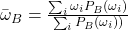$\bar{\omega}_B = \frac{\sum_i \omega_i P_B(\omega_i)}{\sum_i P_B(\omega_i))}$ . We will correlate this with D as a separate measure of classicality.

Other trajectory metrics

When quantifying the correspondence principle, one could compare these Bohmian trajectories with their classical counterparts to see whether they converge. Visually, Bohmian trajectories should approach classical trajectories. To quantify this, one can employ a range of metrics, including an integrated position difference, an integrated velocity difference, and an integrated acceleration difference, given by the following equations:

\Delta r = \frac{\sum_j \left\|\mathbf{r}_B(t_j) – \mathbf{r}_C(t_j)\right\|} {\sum_j \left\|\mathbf{r}_C(t_j)\right\|} \tag{6}

\Delta \mathrm{v} = \frac{\sum_j \left\|\mathbf{v}_B(t_j) – \mathbf{v}_C(t_j)\right\|}{\sum_j \left\|\mathbf{v}_C(t_j)\right\|} \tag{7}

\Delta \mathrm{a} = \frac{\sum_j \left\|\mathbf{a}_B(t_j) – \mathbf{a}_C(t_j)\right\|}{\sum_j \left\|\mathbf{a}_C(t_j)\right\|} \tag{8} \label{eq:da}

Where B is the approaching quantum trajectory, and C is the classical reference trajectory

Research question and hypotheses

This study examines whether classical behavior in Bohmian trajectories emerges due to the principal quantum number or the structure of the wave packet. To do this, we build two packet families with overlapping n ranges, evaluated using the same diagnostics. These include the quantum-to-classical force ratio, the spectral distance D, spectral width, and pointwise trajectory metrics. If classicality depends on n, both families will converge. If it depends on structure, the semiclassically scaled family will converge, while the other does not. Furthermore, we are also seeking to find out whether the different diagnostics will identify the same things.

Significance and purpose

Beyond answering this specific question, establishing a reliable diagnostic that works at accessible n could let us compare packet constructions before reaching the high-n regime. Furthermore, identifying which property of a state controls classical emergence can inform future experiments on what to build, not merely how high to go in n. Circular Rydberg states have been proposed as a platform for quantum simulation and computation²³^,²⁴, and individual circular atoms have now been trapped and optically detected²⁵. Additionally, the ensemble comparison provides a framework which studies the dynamics of the system, and the split-operator method eliminates packet-fidelity issues.

Methodology overview

We started by constructing both Gaussian and Rydberg packets under the soft-Coulomb potential. The Gaussian packets were constructed for n ranging from 3 to 14, while the Rydberg packets were constructed for n ranging from 6 to 13. We evolved each packet using split-operator FFT on a 96³ grid for two orbital periods. We sampled 128 trajectories per n, integrated using the guiding equation for the Bohmian ensemble and directly under the soft-Coulomb potential for the classical ensemble. Finally, we used the Fast Fourier transform on each trajectory’s smoothed acceleration, ultimately comparing the classical ensemble with the Bohmian ensemble. We repeated this for multiple n-values and validated our results with bootstrap confidence intervals, Spearman rank correlation, Pearson coefficient, and leave-one-out analysis.

Scope and limitations

This research only analyzes n values ranging from 3-14 for family A and 6-13 for family B. Thus, we cannot make claims for the high-n range where emergence is typically observed. Additionally, the upper bounds for our convergence may be set by spectral resolution. Furthermore, since we used a soft-Coulomb model, we cannot claim that a true hydrogen atom will follow these trends, although we later show that the resulting force errors are negligible. Additionally, for the Rydberg packets, the softened core, where the difference is most extreme, does not contain any probability for Family B. As previously stated, this research also does not work with true hydrogen spectra, as that would require QED calculations. We will also later discuss how one family loses significantly more samples than another which may impact the results. Finally, since we survey a limited number of n-values, any observed trends cannot be definitively claimed to hold for other values. We must also note that the experimental circular-state literature largely deals with alkali and helium systems¹³^,¹⁵^,¹⁷, with atomic hydrogen realized separately¹⁶; our soft-Coulomb hydrogen model is therefore not a direct model of any existing experiment. We also note that decoherence provides the most popular account of classical emergence, in which environmental monitoring einselects pointer states. When combined with dynamics, this results in the idealized classical trajectory²⁶. Our system is isolated, so the examined effect is complementary to decoherence.

Materials and Methods

The soft-Coulomb model

For this project, to avoid potential divergences, we used the soft-Coulomb potential studied by Hall et al., which makes the potential finite everywhere²⁷. The potential follows the form:

V_{\mathrm{soft}}(x,y,z) = -\frac{1}{\sqrt{x^2+y^2+z^2+a^2}}, \tag{9} \label{eq:vsoft}

where a is a constant. We set a to 0.05, which keeps the potential finite at the origin. We chose this value to make the force error from the Hydrogen atom negligible.

This makes the Hamiltonian of the soft-Coulomb system:

\begin{split} \hat{H}_{soft} &amp;= -\frac{\hbar^2}{2m}\nabla^2 + V(\mathbf{r})\\ &amp;= -\frac{1}{2}\nabla^2 – \frac{1}{\sqrt{x^2+y^2+z^2+a^2}} \end{split} \tag{10} \label{eq:hsoft}

An eigenstate is a wave function that satisfies the eigenvalue equation:

\hat{H}\phi_n = E_n\phi_n. \label{eq:eigen} \tag{11}

When multiplied with the term $e^{(-iE_n t/\hbar)}$ , the time-dependent solution:

\psi_n(\mathbf{r},t) = \phi_n(\mathbf{r})e^{-iE_n t/\hbar} \label{eq:stationary} \tag{12}

solves the time-dependent Schrödinger equation:

i\hbar\frac{\partial\psi}{\partial t} = \hat{H}\psi. \tag{13} \label{eq:tdse}

All results in this paper are for the soft-Coulomb models. Therefore, the extension of the results to a true Hydrogen atom may not be exact. For the circular Rydberg packets introduced in the next subsection, the probability density goes to zero at the origin like $\rho^{2n-2}$ , where $\rho$ is the distance from the z axis. Hence, at the core region, where the softened model makes the largest difference, there is no probability for that family. This research works in atomic units, which sets: $\hbar$ = m = e = 1

Exact time evolution

This research uses direct time evolution of the wave packet, instead of decomposing it into eigenstates. Recalling the time-dependent Schrödinger equation, its solution over a small timestep is:

\psi(t+\Delta t) = e^{-i\hat{H}\Delta t}\,\psi(t) \tag{14} \label{eq:propagator}

However, this exponential cannot be applied directly. The potential energy is simple in position space, while the kinetic energy is simple in momentum space. Thus, the split-operator method that we used splits the evolution into three distinct steps²⁸:

e^{-i\hat{H}\Delta t} \approx e^{-iV\Delta t/2}\,e^{-i\hat{T}\Delta t}\,e^{-iV\Delta t/2} \tag{15} \label{eq:splitop}

The terms that take the steps in potential multiply the wavefunction at each grid point with a phase. Meanwhile, the kinetic energy step uses a fast Fourier transform, multiplying by $e^{(-ik^2\Delta t/2)}$ . Afterwards, it transforms it back. In simple terms, each timestep lets the potential evolve the wavefunction for half a step, lets it spread for a full step, and then applies the potential again for half a step. The splitting is accurate to the second order, and the total probability is also conserved. While applying this method, we detected a normalized probability drift of 3×10⁻¹², which is negligible.

We used a 96x96x96 grid. We chose this because it was the highest resolution we could afford with our computing software. Each box had a half extent according to:

L = n^2 + 6\sigma = n^2 + 12n\quad(\text{family A}) \tag{16}

\label{eq:LA}\\ L = \bar{n}^2 + \frac{6\,\bar{n}^{3/2}}{\sqrt{2}}\quad(\text{family B}) \label{eq:LB} \tag{17}

The two different families are different types of packets we used. We determined these half extents by adding the orbit radius (scales with n $^2$ ) with six packet widths. For packet A, the width is $\sigma$ , or 2n, and for family B, the width is given by $\bar{n}^{(3/2)}/\sqrt{2}$ . Each timestep is equal to the orbital period divided by 4000. We selected 4,000 timesteps because it suited our computational ability, while providing substantially low norm drift and energy drift. This lets us sample 8000 points in total over the two periods. This uniform spacing is needed for the computation of the spectra later.

As mentioned previously, this method practically eliminates norm drift. Furthermore, it does not require projection of a target packet onto eigenbasis. Therefore, the evolved state matches the initial state, and there is no longer any projection-fidelity issues.

Wave packet family A: Gaussian packets with width proportional to n

To start, we choose a particular n-value and find the corresponding radius. By the Bohr Radius formula, we know that

r_n \propto n^2. \label{eq:rn_prop} \tag{18}

For this code, we chose the packet to start on the +x-axis and move counterclockwise. This resulted in a starting position of (r, 0, 0). Next, we assigned a width to the localized wave packet. At this point, our wavefunction is only a function of x, y, and z, without any motion, following the form:

\psi_{\mathrm{blob}}(x,y,z) = \exp\left[-\frac{(x-r_0)^2+y^2+z^2}{4\sigma^2}\right]. \tag{19} \label{eq:blob}

One can note that this is identical to the Gaussian wave packet, where σ controls the width and r₀ represents the radius. We set $\sigma = 2n$ , scaling linearly with n. Note that this is in atomic units, or in this case, in terms of the Bohr radius. Afterward, we add a tangential momentum that points in the +y direction in this scenario. We do this by multiplying by the complex phase factor

e^{ip_y y/\hbar}. \label{eq:phase} \tag{20}

pᵧ is determined by the relation

p_y = \frac{1}{n}. \tag{21} \label{eq:py}

This family of packet is defined by the property that the width grows linearly with n. Since the radius grows with n², the packet becomes narrower (in comparison to radius) as it gets further. This means that, as n increases, the quantum force begins dominating, rather than the opposite. Wave packets of this form also contain a positive-energy component, which is largest at low n. We handle this in a later subsection.

We constructed these wave packets for n values ranging from 3 to 14. 14 was chosen as the upper bound because, beyond 14 we could not achieve satisfactory resolution. We chose 3 as the lower bound because we did not want the width of the packet to be comparable to the orbit radius, since the circular orbit construction would become meaningless.

Wave packet family B: circular Rydberg packets

The second family of wave packets we studied was the Rydberg packets. A Rydberg packet is constructed through a superposition of circular eigenstates, with quantum numbers l = m = n-1. These eigenstates form a circular ring at the desired radius. We used a $\Delta n$ of 1.5, which constrains the weightage of these eigenstates taken into superposition around $\bar{n}$ , the mean principal quantum number. Choosing higher $\Delta n$ , would improve localization, while worsen dispersion over time, and the vice versa is also true. We did not optimize this, and only used $\Delta n$ as 1.5.

Each eigenstate is weighted by a coefficient, and then summed to form the superposition. The weighting coefficient for each eigenstate is given by:

c_n \propto \exp\left(-(n-\bar{n})^2/(4\Delta n^2)\right),\,) \tag{22} \label{eq:cn}

We stopped weighting the eigenstates at $\pm$ 2.5 $\Delta$ n, since the coefficients begin turning negligible. Prior to superposition, we normalized each state on the grid. The packet is also localized on the positive x axis and it rotates counterclockwise. For verification, we found that the angular momentum in the z-direction was equal to $\bar{n}$ -1, to four decimal places. Additionally, the mean radius of the packet was roughly equal to $\bar{n}(\bar{n} + \tfrac{1}{2})$ .

We noticed that, as $\bar{n}$ increases, the quantum to classical force ratio decreased and the localization also increased. Both facts indicate increasing classical behavior. We studied these packets ranging from n = 6 to n = 13. Again, the upper bound was chosen due to resolution limitations. The lower bound was selected because, below 6, n = 1 and n = 2 needed to be included. However, these rings were too small to resolve compared to the larger rings that were also needed.

Bohmian velocity field and trajectory integration

After generating our wave packets, we can assign Bohmian trajectories to them.

The previously stated guiding equation was of the form:

\mathbf{v} = \frac{\hbar}{m}\,\mathrm{Im}\left(\frac{\nabla\psi}{\psi}\right). \tag{23} \label{eq:guiding}

If we define a probability current:

\mathbf{j} = \frac{\hbar}{m}\,\mathrm{Im}(\psi^{*}\nabla\psi). \tag{24} \label{eq:current}

We can write the guiding equation as:

\mathbf{v} = \frac{\mathbf{j}}{\rho}. \label{eq:v_j_rho} \tag{25}

Where ρ is the probability density³

In simpler terms, the particle moves along the probability flow. At each timestep, the gradient of the wavefunction is computed spectrally. This means that we multiplied the momentum-space wavefunction by ik, and then transformed it back. This is the same process we used for the time evolution. To calculate velocities between grid points, we used a trilinear interpolation of the field’s three spatial components.

However, at certain points, the velocity can diverge. This will happen whenever the probability density falls to zero. First, we masked nodes, the points where the wavefunction amplitude vanishes, taken as grid points where the probability density is below 10^-8. At these points, we set the velocity to zero. We also capped the speeds at 10 atomic units. These safeguards only affect particles passing near nodes, and they did not measurably impact the results, since the measured clip fractions were under 4 x 10^-4 and 1.3 x 10^-4, for family A and B, respectively. This means that, out of every ten thousand steps, only few were impacted by the node masking and velocity clipping.

The particle position based on this velocity field is calculated using the Heun predictor-corrector step. For a given particle with a certain position and velocity, we calculate a trial position, which is where the particle would end up if it kept traveling at that velocity for the timestep. At this trial position, a new velocity is calculated, and the final velocity is the average of the two velocities. The final position is the resulting position of this final velocity. Since positions are recorded at every timestep, there are 8,001 points in total for each particle.

Trajectory sampling

Bohmian mechanics gives each particle a definite position. However, since only the initial wavefunction is knowable, we must represent the system with many particles that start off with a distribution governed by this wavefunction. We sample 128 trajectories per n, with their positions determined by the initial wavefunction. We excluded particles that started nearby nodes. The bootstrap confidence intervals that we will later use the sampling uncertainty of this ensemble.

Packet family A (Gaussian packets) contain unbound components. For example, at n = 3, the packet’s mean energy is -0.032 with a spread of ±0.19. This results in some of the ensemble escaping due to having positive energy. Furthermore, the packet disperses over the run, which also carries particles towards the box boundary. Any trajectory that reaches the boundary is excluded from the ensemble for final analysis. For family A, the number of trajectories retained ranged from 62 to 76 out of 128. Meanwhile, for family B, it ranged from 123 to 128. This reflects the Rydberg packets’ resistance to dispersion. We chose to sample 128 particles in order to ensure reasonable confidence intervals can be provided for family A.

Paired classical ensemble and ideal reference orbit

To ultimately compare Bohmian trajectories to their classical counterparts, a single orbit is not enough. Instead, we need a classical partner that gets launched with the same starting position and velocity as each quantum partner we sample. Thus, the partner’s initial velocity is the Bohmian velocity at that point. However, the classical partner is integrated under the same soft-Coulomb force with the velocity-Verlet method²⁹, on the same time grid as the quantum particles. For both quantum and classical particles, the energies are conserved to roughly 1 part in 10⁵. All position, velocity, acceleration, and all spectral metrics are calculated for each partner. With this system, any reported difference can be attributed to the dynamics of the system.

In addition to the ensemble, we still do evaluate an idealized circular orbit as a more global reference. For our classical reference orbit, we modeled an electron that followed the inverse-square force law. The electron orbits the nucleus in a perfect circle with a radius given by the Bohr Radius formula. Once again, the trajectory was run for two orbital periods in order to perform the spectral analysis.

The orbit took the form of:

\mathbf{r}_{\mathrm{cl}}(t) = \left(r_0\cos\left(\frac{2\pi t}{T}\right),\ r_0\sin\left(\frac{2\pi t}{T}\right),\ 0\right). \label{eq:rcl} \tag{26}

Since we set a = 0.05, the classical orbit is, in essence, following a coulombic force, and the circular solution is valid.

The force ratio compared to exact Coulomb is

\frac{F_{\mathrm{soft}}}{F_C} = \left(1+\frac{a^2}{r^2}\right)^{-3/2}. \tag{27} \label{eq:fratio_soft}

Using the Bohr-like radius

r_n = n^2, \tag{28} \label{eq:rn}

and a = 0.05,

\frac{a^2}{r_n^2} = \frac{0.0025}{n^4}. \tag{29} \label{eq:a2rn2}

So the relative force error is approximately

\Delta_F \approx \frac{3a^2}{2n^4}. \label{eq:dF} \tag{30}

For our n range, this force error does not exceed 4.63 x 10^-5 at n = 3, which is negligible. A relative force error of ΔF shifts the circular-orbit frequency by approximately ΔF/2. So, in the worst case, this accumulates to a phase error of 3 x 10^-4.

Accelerations

Before we compute spectra, we must compute each trajectory’s acceleration time series. However, differentiating an already numerically integrated trajectory amplifies jitter into physically meaningless acceleration. To remedy this, we apply a Savitzky-Golay filter, which fits a polynomial to a window of points, smoothing the data³⁰. This polynomial is differentiated to find the derivative, instead of taking a numerical differential. Velocity is the filter’s first derivative, while acceleration is the second. We use a window of 31 timesteps and a cubic polynomial for each trajectory. Since there are 8001 timesteps in total, the window does not influence more meaningful orbital-scale structure. To ensure that our choice in 31 timesteps does not influence the results, we also calculate how different our results would be if we used 51 timesteps instead. Note that we do not need to apply this to the classical partners since their accelerations are given analytically by the soft-Coulomb force.

Spectra and Spectral Distance

Now that we have both the Bohmian and classical trajectories, we can begin analyzing the metrics to quantify their similarity. Spectra are computed from the smoothed acceleration of each trajectory using the following procedure. First, each spatial acceleration component has its time-mean removed and is multiplied by a Hann window³¹. The first step prevents motion of the entire system from getting factored into the spectrum calculation. The latter prevents artificial frequencies from getting introduced. Next, we apply the fast Fourier transform³² to each acceleration component time series. The powers, or the squared magnitudes, for the components are summed to give a final power spectrum. The process follows from this equation, with the same being applicable for y and z:

\tilde{a}_x(\omega) = \mathcal{F}\{a_x(t)\},\quad S_x(\omega) = |\tilde{a}_x(\omega)|^2, \tag{31} \label{eq:fft}

We end up with a power associated with each frequency. The zero-frequency bin is not included, since its content was removed with the mean. The frequency band (0, 6 ω_n] is retained, where ω_n is the ideal orbital frequency. We use this band since it can contain the fundamental frequency, alongside any harmonics. Each spectrum is normalized over this band using trapezoidal integration. The final ensemble spectra are averages of all the individual power spectra. Classical spectra and their ensemble spectra are calculated identically to their quantum counterparts.

We define the spectral difference metric D, as per this equation:

D = \int |S_B(\omega) – S_C(\omega)|\,d\omega \tag{32} \label{eq:D}

This integral takes the L1 distance between two normalized spectra. D = 0 when the spectra are identical, and D = 2 when the spectra share no frequencies. Note that D does not say anything about relative phase, since power spectra carry no phase information. We can also define spectral overlap as 1- D/2, and the variation distance as D/2. Qualitatively, D adds up how much the two spectra disagree, and the overlap is the fraction of the spectra they carry. D must be restricted to [0, 2], since both spectra are normalized and nonnegative.

We use two orbital periods for each sample, so the frequency resolution of each spectra is $\Delta\omega$ = $\omega_n$ /2, where $\omega_n$ is the circular orbit frequency. We chose to use two periods because it’s the minimum amount needed for an acceptable resolution, while still minimizing packet dispersion. This means that, in orbital-frequency units, the frequency resolution is identical. Therefore, we can make cross-n comparisons. To build an intuition for it, we wouldn’t need the same frequency interval for the n = 3 and n = 10 runs, since the former has a larger frequency range. We only need the ratio of the frequency interval and total frequency to be equivalent.

The spectral width metric was calculated by:

\bar{\omega}_B = \frac{\sum_i \omega_i P_B(\omega_i)}{\sum_i P_B(\omega_i)}, \label{eq:wbar}\\ \tag{33}

\sigma_{\omega,B} = \sqrt{\frac{\sum_i P_B(\omega_i)(\omega_i – \bar{\omega}_B)^2}{\sum_i P_B(\omega_i)}}. \label{eq:width} \tag{34}

This metric effectively measures the power-weighted standard deviation of angular frequency. A classical circular orbit has a single dominant frequency, so a narrower spectrum will display closer resemblance to the classical circular orbit. We can also use this as a probe for classicality.

Quantum-force ratio

We can decompose a particle’s acceleration into two contributions. The first is the classical force from the potential we defined. The second is the quantum force that arises from the wavefunction. This idea is expressed in the following equation:

m\,\mathbf{a} = \mathbf{F}_{cl} + \mathbf{F}_Q \tag{35} \label{eq:ma}

where m = 1 in atomic units and F_cl = −∇V. We can calculate F_Q by subtracting the F_cl from the total force (left hand side of the equation). For each n, we report the ratio ⟨|F_Q|⟩ / ⟨|F_cl|⟩, which is the time and ensemble averaged ratio of the quantum and classical forces. Values above unity indicate quantum effects dominating, and values below unity indicate classical dominance.

Radiated-energy check

Before moving on, we would like to address the necessity of a back reaction force from the radiation. As electrons emit light, they radiate away energy. This effect does impact trajectories, but we show that we can neglect the force for the sake of this paper. When a charged particle radiates, the Larmor power scale gives us the radiated power in terms of acceleration and the speed of light²¹:

P \sim \frac{2}{3}\frac{a^2}{c^3}. \label{eq:larmor} \tag{36}

Since a ~ 1/n⁴,

P \sim \frac{2}{3}\frac{1}{c^3 n^8}. \label{eq:larmor_n} \tag{37}

The classical orbital energy scale is:

|E| \sim \frac{1}{2n^2}. \label{eq:Escale} \tag{38}

The period is:

T \sim 2\pi n^3. \label{eq:period} \tag{39}

So the fraction of orbital energy radiated over two periods is:

\frac{\Delta E_{\mathrm{rad}}}{|E|} \sim \frac{16\pi}{3c^3 n^3}. \label{eq:Erad} \tag{40}

For our n range, this fraction has a maximum of 2.4 x 10^-7, at n = 3. This is negligible.

Statistical methods

We use statistical tests to validate our results. First, for every per-n quantity, which includes the motion metrics, the spectral distance, and the quantum-force ratio, we report the 95% bootstrap confidence interval³³. We compute this by resampling the trajectories with replacement (2000 resamples) and recomputing the relevant quantity for each resample. For the spectral distance, each resample re-averages the stored per-trajectory power spectra. Afterwards, it renormalizes and recomputes D. Thus, the ensemble spectrum reflects trajectory-sampling uncertainty.

For any cross-n relationships, we calculate Spearman rank and Pearson correlation coefficients, alongside p-values. Furthermore, we recomputed each coefficient after excluding each point in turn to rule out any outliers as the driving cause.

As mentioned previously, we also reported results with a larger smoothing window (51 timesteps), and those differences are also reported. Since we only sample 12 values for family A and eight for family B, these correlations are merely characterizations of the observed trends rather than definitive claims. We also evaluate which claims survive our different statistical tests.

Results

Packet Characterization

Family	n	Retained Trajectories	⟨p_y⟩ / target	⟨L_z⟩ (target)	⟨E⟩	σ_E
A (Gaussian)	3	66	1.00	3 (3)	-0.032	0.189
A (Gaussian)	4	64	1.00	4 (4)	-0.023	0.131
A (Gaussian)	5	63	1.00	5 (5)	-0.016	0.082
A (Gaussian)	6	72	1.00	6 (6)	-0.011	0.045
A (Gaussian)	7	76	1.00	7 (7)	-0.008	0.023
A (Gaussian)	8	63	1.00	8 (8)	-0.006	0.011
A (Gaussian)	9	72	1.00	9 (9)	-0.005	0.005
A (Gaussian)	10	71	1.00	10 (10)	-0.004	0.004
A (Gaussian)	11	74	1.00	11 (11)	-0.003	0.003
A (Gaussian)	12	74	1.00	12 (12)	-0.003	0.002
A (Gaussian)	13	76	1.00	13 (13)	-0.002	0.002
A (Gaussian)	14	62	1.00	14 (14)	-0.002	0.002
B (Rydberg)	6	123	1.02	5(5)	-0.017	0.015
B (Rydberg)	7	125	1.00	6(6)	-0.012	0.008
B (Rydberg)	8	127	0.98	7 (7)	-0.009	0.004
B (Rydberg)	9	127	0.97	8(8)	-0.007	0.003
B (Rydberg)	10	127	0.97	9 (9)	-0.005	0.002
B (Rydberg)	11	127	0.96	10 (10)	-0.004	0.001
B (Rydberg)	12	127	0.96	11 (11)	-0.004	0.001
B (Rydberg)	13	128	0.95	12 (12)	-0.003	0.001

Table 1 | The packet diagnostics for both packet families for n ranging from 3 to 14 (for packet A) and 6 to 13 (for packet B). By construction, the circular states of family B carry an angular momentum of n̄ – 1.

Table 1 helps us determine the accuracy of the packets. Because they evolved exactly, they all exhibit their intended properties. For example ⟨L_z⟩ always matched its target. Mean energies are slightly less than Coulomb values, with family B’s spread shrinking as n̄ increases. We can also note that family A, at lower n values, can contain positive energies.

Numerical diagnostics

Check	Guards against	Worst case (A/B)
Wavefunction norm drift	Creation/destruction of probability	3 x 10^-12/3 x 10^-12
Velocity clip fraction	Diverging velocities	4 x 10^-4/1.3 x 10^-4
Node-mask fraction	Division by density of zero	0.07/0.36
Boundary-reaching trajectories	Unphysical motion	66 retained out of 128/123 retained out of 128
Classical energy drift	Integrator error	10^-5/10^-5
Smoothing sensitivity (difference in D)	Smoothing choice affecting results	0.01/0.003

Table 2 | Numerical diagnostics, their purposes, and their results

Table 2 collects every numerical safeguard described so far and its measured worst case across all runs of both families: Note that, although the node mask fraction is high, this does not negatively affect the results since particles would not have been sampled at the nodes. Furthermore, the numbers are mostly driven by emptiness beyond the wave packet. Otherwise, all of these diagnostics stay within check, so the results we derived are consequences of dynamics.

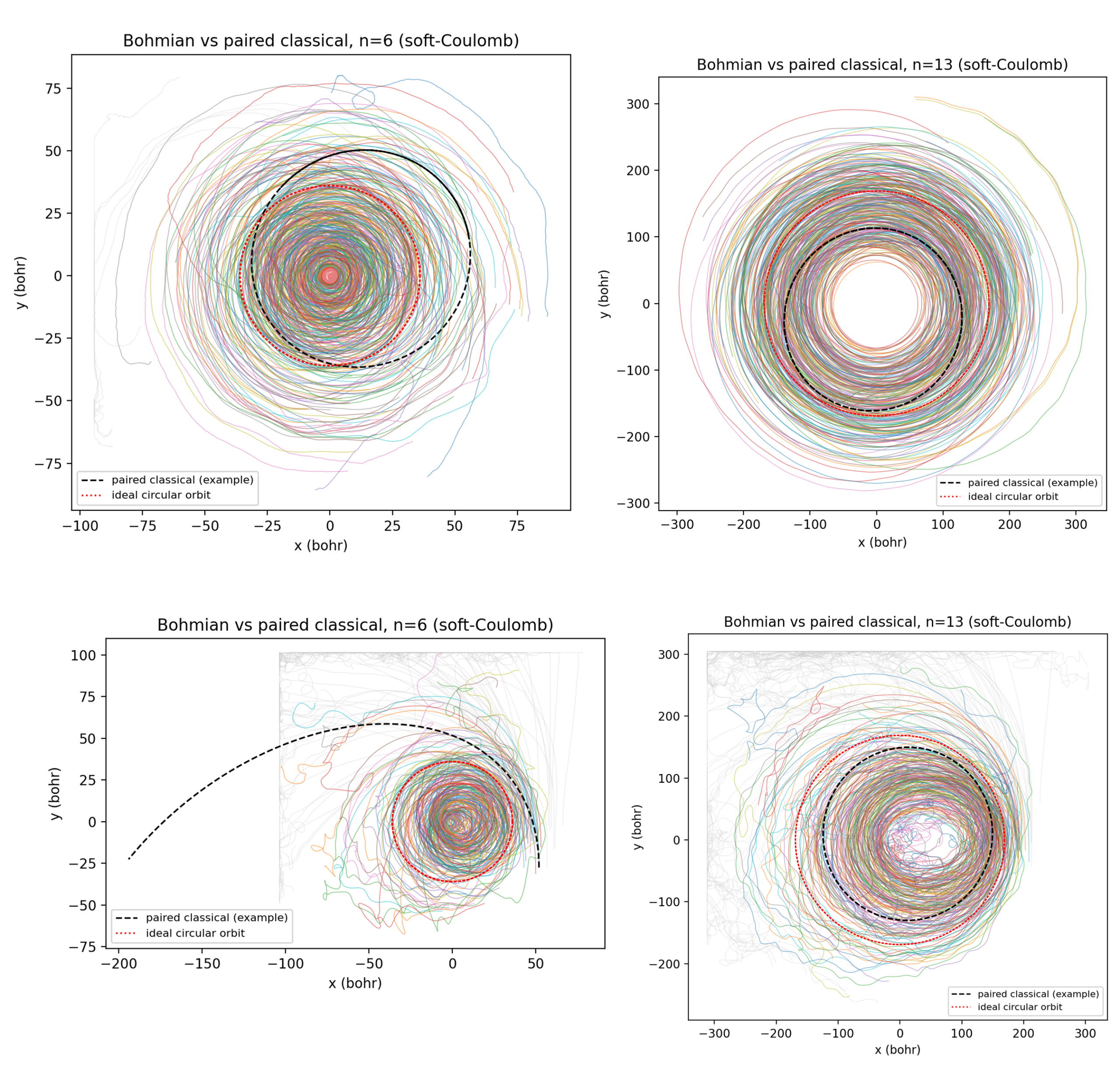
Figure 1 | The trajectories on the x-y plane for the ensemble, for both families A and B at n = 6 and n = 13. Grey paths indicate trajectories that reached the boundary and were not included in the final ensemble. The paired classical orbit is a random orbit from the classical ensemble. The ideal circular orbit shows what an electron’s orbit would look like for that system.

From Figure 1, we can see that Bohmian paths follow a rough circular shape with fluctuations that we attribute to the Quantum force. Overall, family B contained cleaner circular paths, and as n increased for that family, they became increasingly circular. Family A, on the other hand, maintained the same level of circularity throughout.

Family A Results

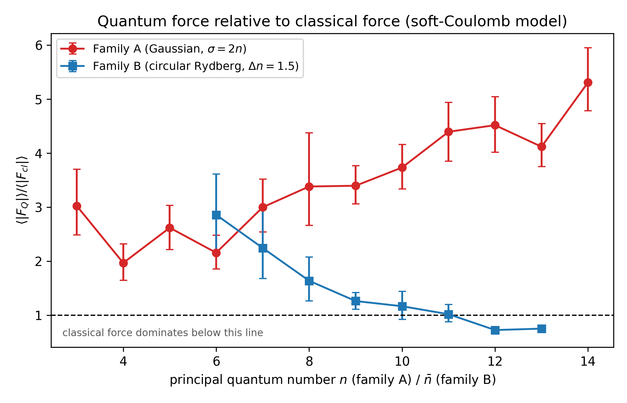
Figure 2 | The quantum force ratio for both families, as n increases

Figure 2 shows the quantum-to-classical force ratio for family A. We can see that the number grows as n increases, specifically, from a mean of 3.02 to a mean of 5.30. We can see that the quantum force is not suppressed as n increases, so from this criterion, family A does not approach classical behavior.

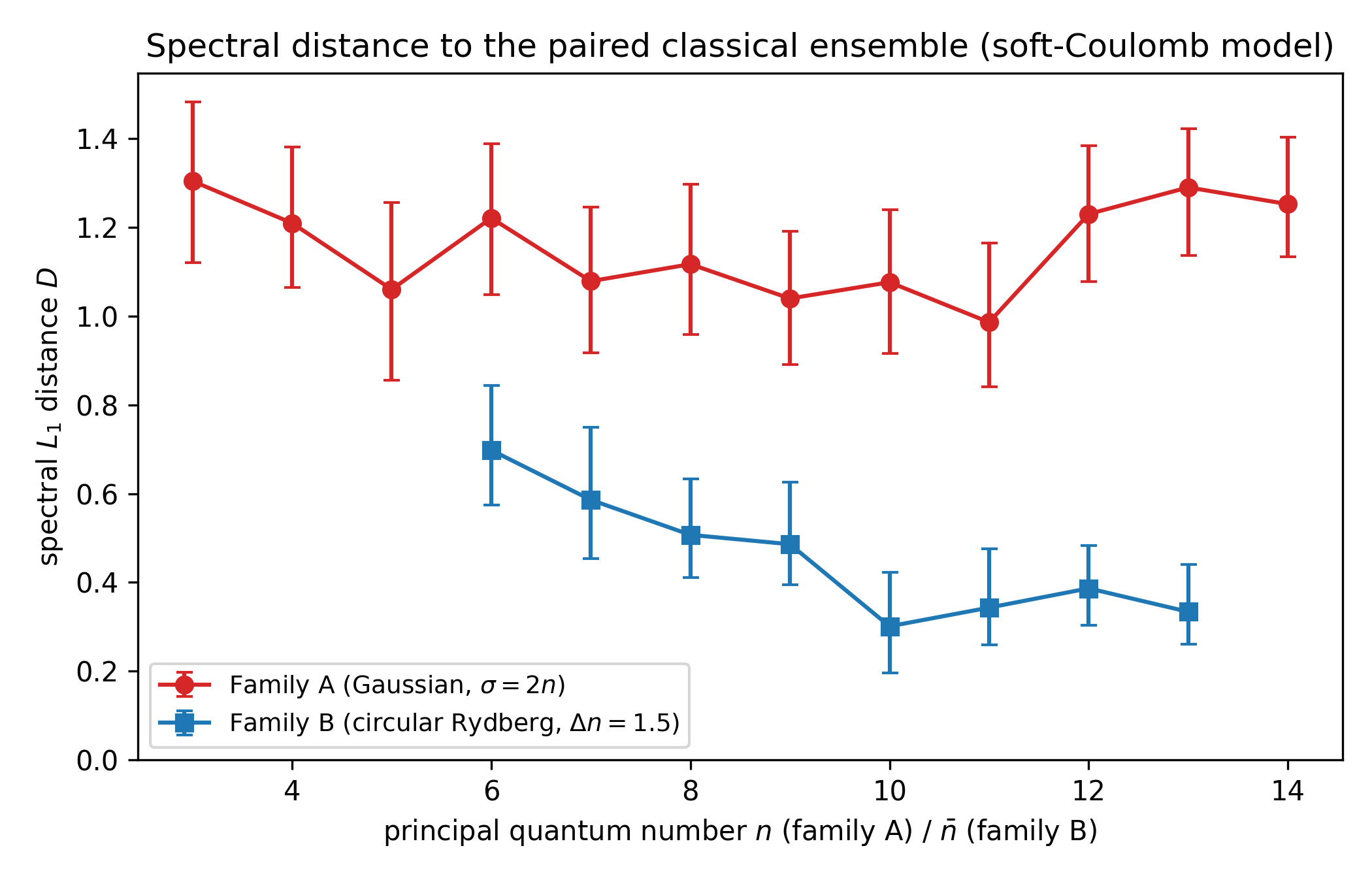
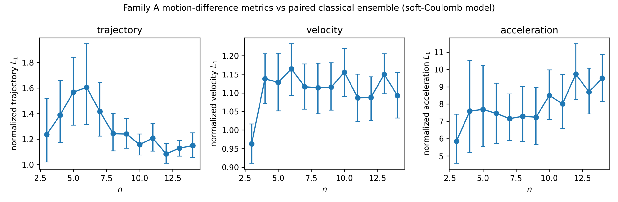
Figure 3 | The spectral distance metric for both families A and B.

Figure 4 | The L1 motion difference metrics for family A.

Figure 3 shows us that the spectral difference varies between 0.99 and 1.30 with uncertainty bars larger than any potential observable trends. We calculated a spearman coefficient of +0.05 which corresponds to a p-value of 0.88. The spectral overlap also remains roughly flat, ranging from 35% and 51%. The total change in D across the range is 0.05, which is less than the confidence interval half-width, 0.16. Therefore, the trend does not exceed the uncertainty. In Figure 4, we can also see that none of the metrics display significant convergence for family A.

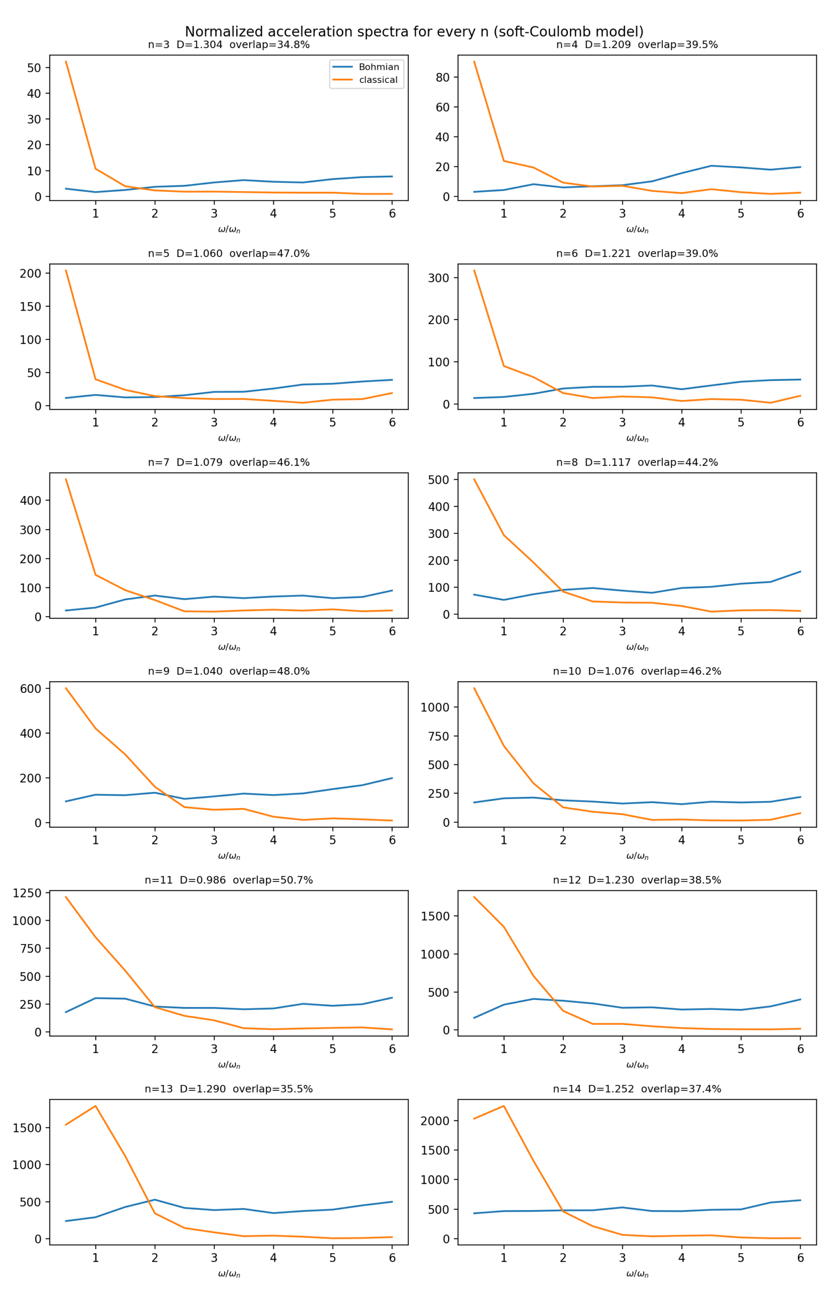
Figure 5 | Normalized Bohmian (blue) and Classical (orange) ensemble-averaged spectra for n from n = 3 to n = 14.

From Figure 5, we can see that, while the classical spectra always shows a peak, the Bohmian spectra remain flat. This effect is what causes the lack of trends we saw in Figure 3.

Previously Identified False Trend

Prior to using the split-operator method, we used projection onto finite eigenstates to evolve our wave packets. Through this method, we identified a downward trend in spectral difference for family A from n = 3 to n = 9. The metric decreased from 1.98 to 1.85. However, we were incorrect in this analysis due to two confounds. First, the finite-basis projection caused fidelity to vary with n. Second, we used a single ideal circular orbit, rather than the sampled ensemble. Furthermore, this paper showed that the Bohmian spectra is more broadband, restricting D’s range to being closer to two. Therefore, the metric was saturated in that area, and going from 1.98 to 1.85 is not significant enough. With exact packets and the paired classical references, this decreasing trend disappeared.

Family B Results

In Figure 2, we can see that the quantum force ratio falls monotonically from 2.86 at n̄ = 6 to 0.72 at n̄ = 13, More significantly, the last value was below 1, indicating that the classical force does begin dominating. This contrasts family A, which has an increasing quantum-to-classical force ratio.

In Figure 3, D decreases from 0.70 at n̄ = 6 to 0.33 at n̄ = 13. This corresponded to the spectral overlap increasing from 65% to 83%. The Spearman coefficient was -0.83 (p=0.010), and the Pearson coefficient was -0.89 (p = 0.003). After leave-one-out analysis, the Spearman ranged from [-0.90, -0.71], and the Pearson coefficient ranged from [-0.95, -0.83]. At the end of the trend, for n̄ > 9, the confidence intervals started overlapping. At the current resolution, we cannot determine whether this is a physical or resolution-limited floor.

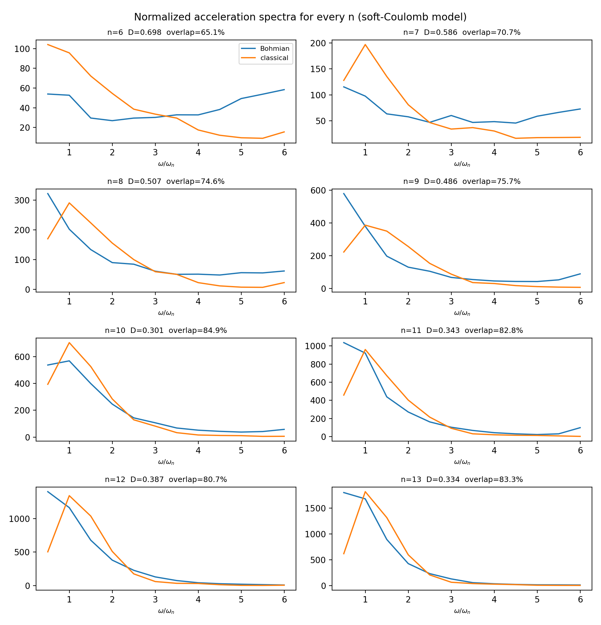
Figure 6 | Spectra of Bohmian (blue) and classical (orange) ensemble-averaged spectra for n̄ ranging from 6 to 13.

Visually, figure 6 shows us that, as n̄ increases, the Bohmian spectra begins replicating the single-peaked classical spectra. When we correlated the spectral difference with the Bohmian spectral width, we found a Spearman coefficient of 0.83 and Pearson coefficient of 0.95. Leave-one-out analysis led to a range of [0.75, 0.96] for Spearman and [0.90, 0.97] for Pearson. This shows that the trend exists within our data, but since we only sample eight points, it is not definitive.

Discussion

In this study, we looked at two separate wave-packet families. For the Gaussian packets with sigma = 2n, the quantum-to-classical force ratio grows. Additionally, there is no spectral distance trend. For circular Rydberg packets with fixed Delta-n, the quantum force ratio goes below 1, and D decreases significantly. Hence, wave-packet structure controls classicality of Bohmian trajectories, and the result from the scaling estimate was confirmed.

However, even for family B, the pointwise velocity metric stayed near 1, despite the forces, spectra, and acceleration converging. Since the classical limit of a quantum state is an ensemble of orbits, not a single orbit²⁰, individual trajectories may remain nonclassical, while the ensemble begins converging. This has been observed directly for radial Rydberg wavepackets, where the packet follows classical motion but the Bohm trajectories differ markedly from the classical dynamics⁹. The pointwise velocity metric shows that trajectory-level convergence is yet to be observed. This answers our second objective.

One limitation of this study is its spectral resolution. Therefore, D’s flattening as n̄ exceeds 10 may be due to a resolution floor. To further assert the results, longer runs are the next step for dispersion-resistant packets. Family A’s results are also bounded by the same resolution limit, since longer runs require larger boxes, which we could not implement. We should also consider the possibility that the decline in D could result from a decreasing relative evolution of the states. Coherent superpositions like this dephase over time and subsequently revive, and the associated timescales grow with n̄¹². By sampling smaller fractions of the total evolution, we may be biasing the results, so to remove this, we must run longer duration runs. Another limitation includes particles that reached the boundary, and were thus not included in the ensemble. Since a lot more particles were sampled for family B, that may impact the results. Additionally, we use the soft-Coulomb model, so we cannot definitively extend these results to Hydrogen. Also, we only tested one Delta-n value for family B, so we do not know its sensitivity to that parameter. Finally, due to our small samples, correlations do not allow us to make strong inferences.

In their 1999 study, Carlsen & Goscinski developed the Bohmian dynamics of this exact circular-Rydberg family. They found pilot-wave theory to be consistent at high quantum numbers with both classical and quantum features⁸. Our study of spectral distance and force ratio provides a quantitative complement to this study. Experiments have observed classical periodic motion for radial and elliptical Rydberg packets¹⁰^,¹¹.

In the future, we could conduct longer runs for packets, increasing spectral resolution; we could conduct the Delta-n sensitivity sweep; we could study elliptical³⁴ and nondispersive Trojan packets, which would require extending the model to include an external driving field³⁵; and work with larger grids for higher n values. We should continue to use the split-operator evolution since it is cheap and removes confounds such as packet fidelity. This study establishes that a quantum system turning classical, not only depends on the n-value, but also the structure of the state.

References

N. Bohr. On the quantum theory of line-spectra, Part I. Det Kongelige Danske Videnskabernes Selskabs Skrifter, Naturvidenskabelig og Mathematisk Afdeling. Vol. IV.1, pg. 1–36, 1918. [↩]
D. J. Griffiths, D. F. Schroeter. Introduction to quantum mechanics, 3rd ed., §9.1. Cambridge University Press, 2018. [↩]
D. Bohm. A suggested interpretation of the quantum theory in terms of ‘hidden’ variables. I. Physical Review. Vol. 85, pg. 166–179, 1952, https://doi.org/10.1103/PhysRev.85.166. [↩] [↩] [↩] [↩]
D. Dürr, S. Goldstein, N. Zanghì. Quantum equilibrium and the origin of absolute uncertainty. Journal of Statistical Physics. Vol. 67, pg. 843–907, 1992, https://doi.org/10.1007/BF01049004. [↩]
S. Goldstein. Bohmian mechanics. Stanford Encyclopedia of Philosophy. https://plato.stanford.edu/entries/qm-bohm/, 2022. [↩]
G. E. Bowman. On the classical limit in Bohm’s theory. Foundations of Physics. Vol. 35, pg. 605–625, 2005, https://doi.org/10.1007/s10701-004-2013-7. [↩]
Z. D. Gaeta, C. R. Stroud, Jr. Classical and quantum-mechanical dynamics of a quasiclassical state of the hydrogen atom. Physical Review A. Vol. 42, pg. 6308–6313, 1990, https://doi.org/10.1103/PhysRevA.42.6308. [↩]
H. Carlsen, O. Goscinski. Dynamics of particles for circular Rydberg states. Physical Review A. Vol. 59, pg. 1063–1069, 1999, https://doi.org/10.1103/PhysRevA.59.1063. [↩] [↩] [↩]
A. Matzkin. Rydberg wavepackets in terms of hidden-variables: de Broglie–Bohm trajectories. Physics Letters A. Vol. 345, pg. 31–37, 2005, https://doi.org/10.1016/j.physleta.2005.07.009. [↩] [↩]
J. A. Yeazell, M. Mallalieu, J. Parker, C. R. Stroud, Jr. Classical periodic motion of atomic-electron wave packets. Physical Review A. Vol. 40, pg. 5040–5043, 1989, https://doi.org/10.1103/PhysRevA.40.5040. [↩] [↩]
Z. D. Gaeta, M. W. Noel, C. R. Stroud, Jr. Excitation of the classical-limit state of an atom. Physical Review Letters. Vol. 73, pg. 636–639, 1994, https://doi.org/10.1103/PhysRevLett.73.636. [↩] [↩]
R. W. Robinett. Quantum wave packet revivals. Physics Reports. Vol. 392, pg. 1–119, 2004, https://doi.org/10.1016/j.physrep.2003.11.002. [↩] [↩]
R. G. Hulet, D. Kleppner. Rydberg atoms in ‘circular’ states. Physical Review Letters. Vol. 51, pg. 1430–1433, 1983, https://doi.org/10.1103/PhysRevLett.51.1430. [↩] [↩]
D. Delande, J. C. Gay. A new method for producing circular Rydberg states. Europhysics Letters. Vol. 5, pg. 303–308, 1988, https://doi.org/10.1209/0295-5075/5/4/004. [↩]
J. Hare, M. Gross, P. Goy. Circular atoms prepared by a new method of crossed electric and magnetic fields. Physical Review Letters. Vol. 61, pg. 1938–1941, 1988, https://doi.org/10.1103/PhysRevLett.61.1938. [↩] [↩]
R. Lutwak, J. Holley, P. P. Chang, S. Paine, D. Kleppner, T. Ducas. Circular states of atomic hydrogen. Physical Review A. Vol. 56, pg. 1443–1452, 1997, https://doi.org/10.1103/PhysRevA.56.1443. [↩] [↩]
V. Zhelyazkova, S. D. Hogan. Preparation of circular Rydberg states in helium using the crossed-fields method. Physical Review A. Vol. 94, pg. 023415, 2016, https://doi.org/10.1103/PhysRevA.94.023415. [↩] [↩]
A. A. Morgan, V. Zhelyazkova, S. D. Hogan. Preparation of circular Rydberg states in helium with n ≥ 70 using a modified version of the crossed-fields method. Physical Review A. Vol. 98, pg. 043416, 2018, https://doi.org/10.1103/PhysRevA.98.043416. [↩]
D. Dürr, S. Römer. On the classical limit of Bohmian mechanics for Hagedorn wave packets. Journal of Functional Analysis. Vol. 259, pg. 2404–2423, 2010, https://doi.org/10.1016/j.jfa.2010.07.011. [↩]
L. E. Ballentine, Y. Yang, J. P. Zibin. Inadequacy of Ehrenfest’s theorem to characterize the classical regime. Physical Review A. Vol. 50, pg. 2854–2859, 1994, https://doi.org/10.1103/PhysRevA.50.2854. [↩] [↩]
J. D. Jackson. Classical electrodynamics, 3rd ed., §14.2. Wiley, 1999. [↩] [↩]
C. Cohen-Tannoudji, J. Dupont-Roc, G. Grynberg. Atom-photon interactions: Basic processes and applications, Wiley, 1992. [↩]
T. L. Nguyen, J. M. Raimond, C. Sayrin, R. Cortiñas, T. Cantat-Moltrecht, F. Assemat, I. Dotsenko, S. Gleyzes, S. Haroche, G. Roux, T. Jolicoeur, M. Brune. Towards quantum simulation with circular Rydberg atoms. Physical Review X. Vol. 8, pg. 011032, 2018, https://doi.org/10.1103/PhysRevX.8.011032. [↩]
S. R. Cohen, J. D. Thompson. Quantum computing with circular Rydberg atoms. PRX Quantum. Vol. 2, pg. 030322, 2021, https://doi.org/10.1103/PRXQuantum.2.030322. [↩]
B. Ravon, P. Méhaignerie, Y. Machu, A. D. Hernández, M. Favier, J. M. Raimond, M. Brune, C. Sayrin. Array of individual circular Rydberg atoms trapped in optical tweezers. Physical Review Letters. Vol. 131, pg. 093401, 2023, https://doi.org/10.1103/PhysRevLett.131.093401. [↩]
W. H. Zurek. Decoherence, einselection, and the quantum origins of the classical. Reviews of Modern Physics. Vol. 75, pg. 715–775, 2003, https://doi.org/10.1103/RevModPhys.75.715. [↩]
R. L. Hall, N. Saad, K. D. Sen, H. Ciftci. Energies and wave functions for a soft-core Coulomb potential. Physical Review A. Vol. 80, pg. 032507, 2009, https://doi.org/10.1103/PhysRevA.80.032507. [↩]
M. D. Feit, J. A. Fleck, Jr., A. Steiger. Solution of the Schrödinger equation by a spectral method. Journal of Computational Physics. Vol. 47, pg. 412–433, 1982, https://doi.org/10.1016/0021-9991(82)90091-2. [↩]
W. C. Swope, H. C. Andersen, P. H. Berens, K. R. Wilson. A computer simulation method for the calculation of equilibrium constants for the formation of physical clusters of molecules: Application to small water clusters. The Journal of Chemical Physics. Vol. 76, pg. 637–649, 1982, https://doi.org/10.1063/1.442716. [↩]
A. Savitzky, M. J. E. Golay. Smoothing and differentiation of data by simplified least squares procedures. Analytical Chemistry. Vol. 36, pg. 1627–1639, 1964, https://doi.org/10.1021/ac60214a047. [↩]
F. J. Harris. On the use of windows for harmonic analysis with the discrete Fourier transform. Proceedings of the IEEE. Vol. 66, pg. 51–83, 1978, https://doi.org/10.1109/PROC.1978.10837. [↩]
J. W. Cooley, J. W. Tukey. An algorithm for the machine calculation of complex Fourier series. Mathematics of Computation. Vol. 19, pg. 297–301, 1965, https://doi.org/10.1090/S0025-5718-1965-0178586-1. [↩]
B. Efron. Bootstrap methods: Another look at the jackknife. The Annals of Statistics. Vol. 7, pg. 1–26, 1979, https://doi.org/10.1214/aos/1176344552. [↩]
M. Nauenberg. Quantum wave packets on Kepler elliptic orbits. Physical Review A. Vol. 40, pg. 1133–1136, 1989, https://doi.org/10.1103/PhysRevA.40.1133. [↩]
I. Bialynicki-Birula, M. Kaliński, J. H. Eberly. Lagrange equilibrium points in celestial mechanics and nonspreading wave packets for strongly driven Rydberg electrons. Physical Review Letters. Vol. 73, pg. 1777–1780, 1994, https://doi.org/10.1103/PhysRevLett.73.1777. [↩]