

Abstract
Large language models are increasingly being used in creating investment strategies. However, most studies that create a pipeline, feed news and financial reports in a single prompt to the LLMs. This can reduce relevant signals. To address this limitation, we developed a two-stage filtering framework which uses news articles to select a candidate stock pool. It then uses financial reports to further improve and finalize the portfolio. Across 2759 matched portfolio runs, moderate two-stage filtering consistently outperformed an unfiltered single-pass baseline using the same information. These runs utilized three OpenAI models, ten filtering configurations, and rolling 12-month evaluation windows. For GPT-5.1, the best performing setup narrowed 20 candidates to 10, raising the mean ROI from 45.7% to 60.6%. The risk profile stayed around the same with an annualized volatility of 28.1% compared to 27.8%. The risk profile also had a maximum drawdown at -23.2% compared to -22.4%. The median Sharpe ratio increased from 1.34 to 1.70. That filtered configuration outperformed the matched baseline in 22 out of 27 window comparisons. The results demonstrate that the size of the initial candidate pool matters. Moderate sized pools of ten to twenty candidates outperformed, while oversized pools performed below baseline. Unlike the unfiltered baseline, the filtered portfolios also beat an equal-weighted portfolio of the eligible universe and the randomized portfolios with the same number of holding counts. These results show that the strategy relies on selection skill rather than just sector exposure. Comparisons with the S&P 500 and sector indices are included as additional benchmarks for context, but they are not the primary comparisons because the eligible universe is technology-heavy. Therefore, the results suggest how these models ingest information is a high design priority for LLM investment systems.
Keywords: large language models, investment strategy, two-stage filtering, portfolio construction, financial news analysis, information structuring
Introduction
Background and Context
Strong financial analysis requires using qualitative sentiment. This sentiment comes from earnings reports and news sources, and it is done using quantitative metrics like historical price, volume, and risk profiles1,2. LLMs are progressively applied to financial markets to generate data points that suggest the future movement or trend of a certain economy. Some of these data points include buy, hold, or sell recommendations, and these are found by combining information from news, earnings reports, and regulatory filings3,4,5. This application capitalizes on LLMs’ ability to understand natural language.
Most LLM-based investment research targets short-term periods, and some examples are high-frequency trading and single-day price prediction3,4,6. More and more research explores long-term periods6,7 but most of these studies do not prevent look-ahead bias. Look-ahead bias can be prevented by restricting the model to information available at the simulated decision date. Additionally, only a few studies use holding periods that are longer than one quarter6.
This gap motivates this work, which is whether a structured LLM pipeline is able to generate reliable strategies. This is done over 12-month periods and under a forward-usable protocol, where every decision only uses information that is available at that date. The protocol, not the specific model, transfers because the models themselves came out after the earliest simulation dates.
LLMs can summarize8, extract information, and generate content. This supports market trend monitoring, risk factor identification, and investment decision support1,2. As these models have scaled, they are more capable of processing varied financial data1,9. However, since it is unclear, it is difficult to determine if outputs reflect genuine reasoning or coincidences LLMs learned from training10,11. Therefore, principled deployment frameworks matter1,12 because undetected biases spread into important decisions10,13.
Large Language Models in Financial Forecasting
LLMs combine varied financial data so they can extract predictive market signals3,5,14. Combining them with conventional forecasting improved predictive accuracy, and the cause of this was capturing relationships between news sentiment and price movements3,14,15. This approach combines digital text representations from documents and the LLM to estimate investor sentiment, and broad macroeconomic conditions14,16. This reduces manual overhead and allows for more scalable modeling pipelines14,16.
Multi-Agent LLM Systems for Trading
LLMs are not confined to single-model deployments. They can also serve as components of multi-agent trading systems. In these systems, specialized agents interact with each other to simulate market dynamics and refine portfolio strategies4,17,18,19. Agents can retain historical context and adapt as conditions evolve because of layered memory and designs that are different based on their role20,21. Because of this, multi-agent systems often outperform systems with a single agent, and strategy diversity reduces overfitting seen in isolated backtests18,22. In these multi-agent systems, each agent is assigned a different function, such as allocation, risk assessment, or monitoring4,17,23. Some examples of multi-agent systems include 3S-Trader24, AlphaAgents25, FinRobot26, and tool-augmented multimodal foundation agents27. They coordinate multiple LLMs to score candidate stocks, construct portfolios, and refine strategies from historical performance. However, it comes at the cost of considerable system complexity.
Sentiment Analysis and Market Dynamics
Many prior works have focused on LLMs estimating investor sentiment and predicting market changes using news articles and social media3,14,28. Some studies have found that pre-training models on larger financial datasets improves their ability to interpret specialized terminology and rhetorical intent, skills that are integral to predicting price movements from text3,29, and these models have been reported to identify stock trend reversals early3,28. The ability for LLMs to process unstructured data at large scales allows for quicker, highly detailed strategies1,23, which furthers foundational work that shows how media content can yield quantifiable sentiment signals that have measurable impact on equity prices3,28.
Self-Improving and Feedback-Driven Financial LLMs
More so than single-pass designs, agent systems that are self-improving and feedback-driven have reported higher gains in automated trading21,30. These systems iteratively modify their strategies according to feedback from simulated markets or accumulated market knowledge19,30, and modeling portfolio management as a sequential decision problem balances exploring new strategies and reusing established ones30. For non-static markets, this adaptability is especially useful4,21.
Benchmarks, Evaluation, and Bias
Systematic benchmarking is a vital tool to enable more objective analysis of financial LLMs29,31,32. One part of this is the use of standardized datasets, which allow comparison between different models on tasks such as textual comprehension, sentiment extraction, and portfolio optimization29,32. However, models must be able to perform under live-market pressures, where results from preexisting datasets can be shown to be due to favorable evaluation conditions6,19,32. Therefore, benchmark development is essential to separate genuine improvements from results inflated by methodological issues3,6,32.
One important concern is evaluation bias. A rigorous testing framework, FINSABER6, was introduced to address three typical problems: survivorship bias (not testing on stocks that were delisted or went bankrupt), look-ahead bias (using information that chronologically would not have been available at the time of the decision), and data-snooping bias (retesting on the same data until favorable results arise by chance). When FINSABER was applied over 20 years of data across a larger range of stocks, many popular LLM structures’ advantages were shown to be much weaker or non-existent across different market regimes: cautious in bull markets and aggressive in bear markets. These findings are the reason for our evaluation design: longer horizons, matched comparisons, and specific safeguards for all three biases.
Together, these studies show LLMs have the capability for competitive strategy generation. However, there is a lack of focus on the structure of information delivery compared to factors like larger architectures, multi-agent systems, reinforcement learning, and sentiment extraction. This issue begs the question: can restructuring the information presented to an LLM systematically improve long-term investment decision-making?
Problem Statement and Rationale
There are several important limitations that have historically limited LLMs from investing and finance in general.
One of the most significant limitations is their weakness with calculations11. LLMs are prone to make arithmetic errors, which limits their usefulness in financial tasks that require a considerable amount of quantitative analysis. They cannot fully replace analysts who rely on financial modeling and their professional judgement.
Hallucination is another major limitation. LLMs can present incorrect or invented information with an alarmingly high degree of confidence13. In investing, this could lead to recommendations based on inaccurate figures or completely nonexistent reports.
Subtler errors, such as misinterpreting a company’s performance or slightly misstating a fact, are even harder to detect. These mistakes can worsen over time as they will create a compounding effect.
Bias from pre-training may also create problems. A model’s training data may include information from after the historical period being analyzed. Therefore, it can unintentionally use future knowledge during backtesting. This bias can make an investment strategy appear more successful than it actually would have been at that time.
This paper addresses two related gaps. The first gap is that there is limited evidence on how well LLM-based investment strategies perform over several months, since much existing research generally focuses on short-term results. Second, processing many information sources can lead to confusion and also inconsistent investment decisions.
Significance and Purpose
This paper proposes a two-stage pipeline for long-term investment strategy generation. It decomposes the investment strategy generation task into a news-based candidate selection stage and a financial report validation stage.
In the candidate selection stage, the LLM identifies candidate stocks from curated financial news. In the financial report validation stage, the LLM reads company reports for each candidate and produces a smaller, more accurate portfolio. Having this sequential, rather than a simultaneous evaluation of information sources is the main methodological contribution of this paper.
Objectives
The paper makes three key contributions. It introduces a two-stage news and financial report architecture first, for LLM-driven long-term investment strategy generation. The architecture separates qualitative from quantitative reasoning in a principled way, making each stage auditable on its own. And allows differences in performance to be attributed to a specific stage. This paper also provides extensive empirical validation, focused on advanced frontier models.
With moderate filtering configurations, the mean ROI reaches up to 60.6%, as these configurations maintain a mid-sized candidate pool and roughly halve it between stages with volatility and maximum drawdown similar to the unfiltered baseline (28.1% against 27.8%, and −23.2% against −22.4%), outperforming the baseline in 74–82% of matched evaluation windows across four well-sized configurations, and exact confidence intervals are reported in the Results. These configurations also outperform an equal-weighted portfolio of the eligible universe and random matched-size portfolios, but the unfiltered baseline doesn’t; the S&P 500 is included for context only. The paper presents a systematic sensitivity analysis, looking at returns and consistency across ten pipeline configurations. The analysis shows that moderate filtering consistently improves on single-pass methodologies, but aggressive over-filtering degrades performance, as it forces the model to draw from an oversized candidate pool it can’t fill with strong companies. The optimal filtering threshold depends on the model, and for the tested target sizes, the best configuration has a Stage One pool roughly twice the size of the target portfolio; given the coarse configuration grid, this is presented as a working hypothesis rather than a rule.
Scope and Limitations
This study focuses on long-only, buy-and-hold portfolios selected from large-capitalization technology and semiconductor equities, evaluated across rolling 12-month periods using three model variants (GPT-4o, GPT-4o-mini, and GPT-5.1). Returns are measured before accounting for transaction cost and taxes, and all evaluation windows respect each model’s training cutoff. Broader limitations are addressed in the Discussion section. Throughout the paper, “long-term” denotes these 12-month buy-and-hold horizons: long relative to the intraday-to-quarterly horizons that dominate the prior LLM-trading literature, though medium-term by traditional investing standards. Rather than relying on a predefined ticker list, the model freely selects candidate companies directly from screened news coverage in every filtered step. As a result, the active investment universe is open and emerges from contemporaneous news rather than a curated survivor list. A fixed set of large-capitalization technology and semiconductor names is used only for the unfiltered single-pass baseline and serves as the set for the benchmark comparison.
Methods
Overall Framework Overview
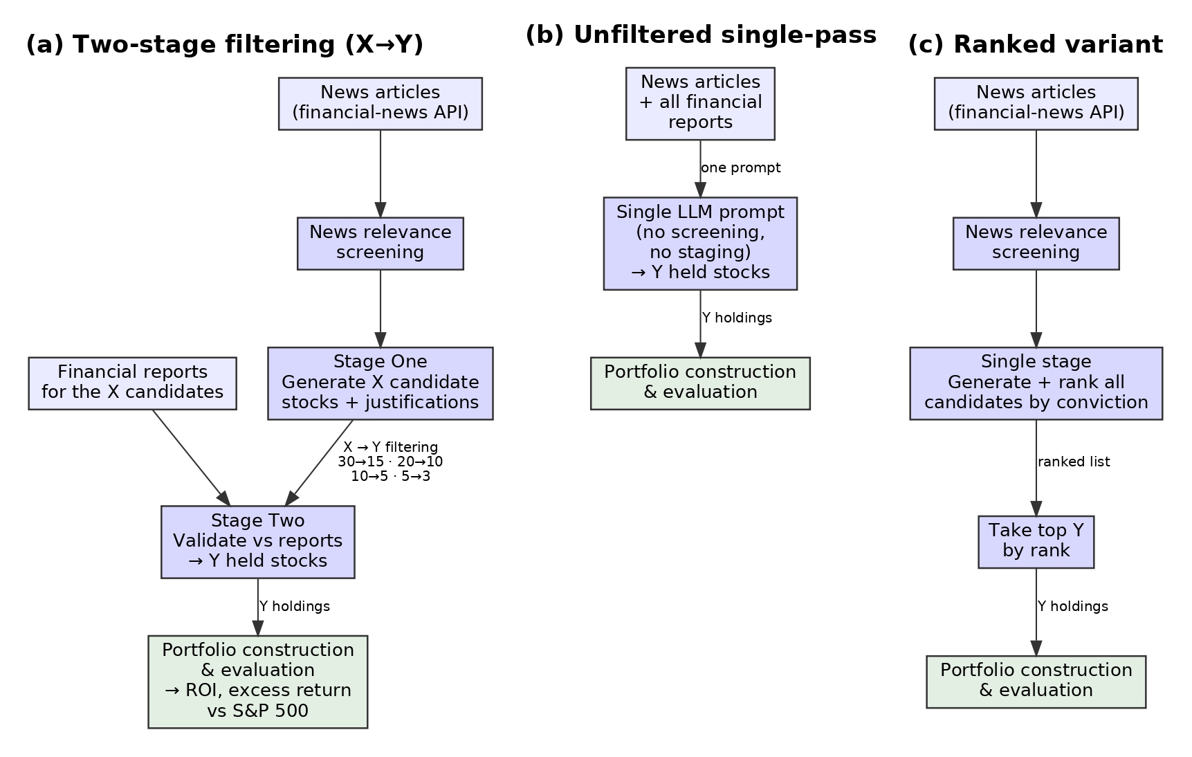
The framework’s architecture is illustrated in Figure 1. The main principle of this design is that we separate the feeding of information to the LLM in different steps based on the purpose. While typical approaches feed news articles, financial reports, and other market information all at once to the LLM, we believe this approach dilutes relevant signals between different sources. By splitting the sources into different steps, we can separate information used for opportunity discovery from information for financial validation.
This framework has two stages with some surrounding steps. First, news articles from the New York Times archive are collected from a fixed pre-analysis window. We then feed this data to an LLM to receive a list of initially nominated stocks with specific qualitative justifications based on trends and events described (Stage One of the framework). Afterwards, financial reports for each candidate are collected from the Alpha Vantage API and fed to the LLM, producing a smaller set of final recommendations (Stage Two). These final selections and their allocation weights assigned by the LLM are used to build a long-only portfolio that we evaluate over a predefined horizon. The notation X→Y denotes this structure: X stands for the number of initially nominated candidates, and Y is the number of stocks in the final portfolio.
An exception to this generalized structure is the Ranked configuration. Unlike the typical stock filtering framework which outputs a fixed number of stocks each step, the Ranked configuration instead ranks a list of stocks with no defined limit each step. This leads to an LLM-defined final portfolio size.
While the portfolio is generated by the LLM, quantitative analysis is done deterministically in code. LLMs are typically not consistent when making calculations11,13, so this approach prevents incorrect return and risk calculations.
A similar issue with LLM calculation inconsistency arises with the LLM providing allocation percentages that sum up to numbers different from 100%. To correct this, we renormalize the percentages by multiplying each percentage by 100 divided by the sum of the LLM’s allocations. This preserves the LLM’s relative proportions while ensuring the weights sum to 100.
To evaluate the specific effect of the filtering framework on the performance of the generated portfolios, we tested multiple configurations. These include variations of the X→Y structure (30→15, 30→10, 30→5, 20→10, 20→5, 10→5, 10→3, and 5→3), the Ranked configuration, and an unfiltered baseline. The unfiltered baseline is representative of the typical method of information processing for the LLM (simultaneously providing all types of data rather than sequentially).
Data Sources
The three main categories of data used in this study are news articles, financial reports, and historical market prices. The news articles were obtained through the New York Times Article Search API, and the financial reports were acquired through Alpha Vantage reports of major tech companies, in which both were cached locally. For each decision date, news data is collected from a fixed 24 month window ending at that date. Article publication timestamps are converted to Coordinated Universal Time (UTC) and compared to the publication date only. Duplicated or republished stories are removed by tracking the exact headline, in which the first occurrence of each is kept.
Financial reports consist of quarterly income statements, balance sheet statements, and cash-flow statements, which are retrieved for each stock that passes Stage One. This provides structured company-level data to the LLM in Stage Two which is used to validate the candidate list. A report’s fiscal period end alone does not establish that the information was available on the given decision date. Therefore, a report is only admitted if it was available strictly before that date. The report is considered available based on the later date between the statutory filing deadline, and any filing date supplied by the source. The deadlines are 45 days for quarterly filings and 75 days for annual filings. These deadlines cover for all filer classes for quarterly reports and annual filers, except for non-accelerated filers. The deadline for non-accelerated filers can extend to 90 days. This represents a limited edge case because the selected stocks are primarily dominated by large-capitalization filers subject to the shorter deadlines. Reports dated on the decision date are also excluded because filings accepted after 17:30 Eastern Time are available on the following business day. As a result, the most recent quarter is withheld when a decision date belongs to its filing window. For the unfiltered baseline, financial reports for the full set of stocks selected by any configuration are provided with all available news articles.
Market data consists of daily adjusted closing prices for individual stocks and benchmark indices. This data is only introduced after the LLM finalized the recommendations. Isolating the market prices from the recommendations prevents look-ahead bias, as future data can influence the model’s decisions. All return and risk metrics are computed externally using deterministic formulas.
News Article Relevance Screening Process
For raw news articles, many of the elements are irrelevant to the investment strategies such as opinion pieces, general technology discussion, and political commentary without market implications. Therefore, these articles are filtered out prior to the strategy generation. To accomplish this, the LLM is prompted to label each article as financially relevant or irrelevant. Due to this there is no need for manual review or rule-based matching. This keeps the screening consistent and scalable. We then screen batches of articles for direct market relevance only: earnings announcements, major corporate events, regulatory changes, macroeconomic indicators, and industry-level shifts.
By filtering out the screened articles and putting them into a selected database, they are reused downstream, letting only a small, high-quality input data set drive the strategy generation, and reducing the influence of non-relevant or misleading data. Across the entire training set, the filter kept 1,799 of 13,183 unique articles (13.6%) under strict investment-relevance criteria. The validation sample described below is sourced from a single screening run of 1,382 articles, of which 110 (8.0%) passed.
To check the screen against human judgment, we blind-labeled a stratified sample of 180 articles (70 passed, 110 rejected) without seeing what the screen decided. Against that first rating, the screen hit 100% precision (95% Wilson CI [94.8, 100]). Re-weighting to the 13.6% corpus pass rate gives an estimated recall of 26.2% and a false-omission rate of 44.5%. One rater is only one standard, so we brought in a second one. The rater was blind to both the screen’s decisions and the first rater’s labels, and independently label the same 180 articles. The two agreed on 83.3% of them (95% CI [77.2, 88.1]; Cohen’s κ = 0.67, or 0.57 re-weighted to the corpus pass rate.)
The disagreement was highly skewed. In 29 cases the first rater called an article relevant and the second did not. Only one case went the other way (exact McNemar p = 6×10⁻⁸). So the two raters mostly differ on where they draw the line, but not on their consistency. And the term “relevant” admits a wider or narrower reading than our rubric fixes. Under the first rating, 52.1% of the corpus is investment relevant. Under the second, 31.9%.
Precision moves correspondingly, 95.7% (95% CI [88.1, 98.5]) under the second rater against 100% under the first, with false omission rates of 21.8% and 44.5% and re-weighted recalls of 41.0% and 26.2%.
The screen passes 13.6% of the corpus, which is stricter than the human readings. This means on neither reading does it let much off-topic materials through into the downstream stages. Its recall, on either reading, is well below one, and we flag that as a limitation. In normal operation, the screen runs without human adjudication.
Bias and Hallucination Mitigation
Hallucinations and implicit bias are known aspects of large language models, and these problems are particularly impactful when an LLM is prompted with open-ended tasks or incomplete constraints13. To prevent this, several safeguards have been integrated into the framework.
First, we ensure information fed to the LLM is heavily restricted to prevent any temporal leakage. The news articles fed to the LLM are restricted based on the criteria of publication date being before the evaluation period, and financial reports are restricted based on the date they would have been open to the public under the rule mentioned in Data Sources.
Secondly, we ensure a more subtle issue does not pass by, that being knowledge cutoff dates. Some of the earlier evaluation periods we selected started before a model’s knowledge cutoff, so even with the restriction on data fed to the model there existed a risk of inherent knowledge guiding the model. To solve this, we simply do not run an evaluation period on a certain model if their knowledge cutoff conflicts.
Finally, by asking the model for a justification of each recommendation, we encourage it to base its selections on the input information rather than choosing stocks arbitrarily. This also allows us to see whether a model may have hallucinated in a run. In the runs reported here, this check was used to audit the model’s output, and no recommendation was removed by it.
Portfolio Construction
All portfolios are buy-and-hold year-long investments, with no short selling, leverage, or derivatives used. Positions are held throughout the evaluation window without rebalancing.
Portfolio values are calculated using adjusted closing prices to account for factors such as stock splits causing a stock to appear to drop in price and dividends being reinvested rather than kept. This allows for a view of the actual total return rather than just price changes. Each portfolio starts with the same amount of value, and the return is calculated from the closest trading day on or after the start of the period to the closest trading day on or before the end. Using the SPY exchange-traded fund to represent the S&P 500 index also prevents the issue with dividends not being included in the index, ensuring accurate comparison.
Permutation Analysis Framework
Model robustness was tested through a large permutation analysis across various models, temperatures, filtering setups, and evaluation windows.
We compared three models: GPT-4o, GPT-4o-mini, and GPT-5.1. All generations were obtained through the OpenAI API using the aliases gpt-4o, gpt-4o-mini, and gpt-5.1.
For GPT-4o and GPT-4o-mini, we tested temperatures of 0.3, 0.4, and 0.5 across each of the ten filtering settings described in the framework overview.
We handled GPT-5.1 differently as we ran three generations for each window and configuration, but the OpenAI API did not allow custom temperature settings for the GPT-5.1 family. All GPT-5.1 runs therefore used the default settings. While these runs do use the same three temperature labels in the dataset, they should be treated as separate runs under the same settings. We do not report temperature-level results for GPT-5.1.
In the X→Y notation (which we used throughout the paper), where X represents the Stage One candidate pool size, while Y represents the final Stage Two portfolio size. The unfiltered baseline uses a single pass, while the Ranked configuration ranks the Stage One candidates without setting a fixed portfolio size.
Other settings apply different levels of filtering. For example, candidate pools of 10 or 20 stocks may be reduced to smaller portfolios, as in 20→10, 10→5, 10→3, or 20→5. More aggressive settings begin with 30 candidates and reduce the final portfolio even further. These labels describe the setup only and do not imply anything about performance.
We used model-specific knowledge cutoffs to limit any lookahead bias. We excluded any window beginning before a model’s reported cutoff.
The cutoff used for GPT-4o and GPT-4o-mini was October 2023. For GPT-5.1, we used September 30, 2024.
These restrictions left 13 monthly windows for GPT-4o and GPT-4o-mini, running from June 1, 2024 to June 1, 2025, and nine for GPT-5.1, from October 1, 2024 to June 1, 2025.
In total, the dataset contained 2,759 matched portfolio runs: 921 from GPT-4o, 1,212 from GPT-4o-mini, and 626 from GPT-5.1. The full breakdown by each specification (model, config, window, etc.) is included in the Supplementary Information.
Win rates were calculated using matched cells. For GPT-4o and GPT-4o-mini, we compared the mean ROI of each configuration with the unfiltered baseline from the same specifications.
For GPT-5.1, its three groups were repeated runs at its default settings rather than at separate temperatures.
This gave 27 matched comparisons per configuration for GPT-5.1 and up to 39 for GPT-4o and GPT-4o-mini.
Matching each configuration with an unfiltered baseline from the same model and market period made the comparison more direct, which makes it easier to analyze. Therefore, differences are less likely to come from the model used or from the particular evaluation window.
Evaluation Methodology
Performance of strategies is evaluated based on benchmark-relative, comparative metrics, and return-based metrics.
The primary performance measure is return on investment (ROI), which is calculated over a fixed 12-month evaluation period. The portfolio performance is compared against the S&P 500 index over the same period. This allows for the calculation of benchmark-relative excess return (reported as raw excess return over the index). This is different compared to risk-adjusted alpha which measures excess return after accounting for the level of risk taken.
Baseline win rates are calculated by comparing each filtering configuration with an unfiltered baseline using the same model, temperature, and evaluation window. The win rate is the percentage of windows in which the filtered configuration achieves a higher ROI. This provides us with a direct measure of whether sequential filtering actually improves portfolio quality.
Portfolio risk is measured using daily portfolio values based on each portfolio’s tickers, weights, and dates. We report annualized volatility, maximum drawdown, and the Sharpe, Sortino, and Calmar ratios alongside each return figure. Run-to-run variability is measured separately using standard deviation and coefficient of variation (CV). Since CV measures variability relative to average return, it helps us compare both performance and consistency across different runs.
Finally, we combined the results across all models, temperatures, configurations, and evaluation windows to identify the performance trends and examine how model capability interacts with the way the information is organized.
Statistical Limitations
Some configurations use the same evaluation windows, source articles, and some of the same candidate portfolios. Because of this, the results are not completely independent. To account for this, the statistical test compares each configuration with its matched baseline within the same window. The tests do not assume a specific distribution of the data. The p-values are mainly used to show how strong the differences are between the configurations and their baselines. They should not be treated as exact error rates that would apply if all of the observations were independent. The number of runs also varies across GPT-4o-mini: the September 2024 window had many more runs than the other windows, making up 309 of the model’s 1212 total runs. As a result, this one window has a larger effect on the model’s overall average. This does not affect the paired tests because each configuration is compared with its baseline within the same window before the results are combined.
Results
Key Findings
The structured two-stage filtering method increased GPT-5.1’s mean ROI to 60.6%, compared to the 45.7% for unfiltered single-pass prompting. This was a gain of 14.9 percentage points. Risk remained stable with an annualized volatility of 28.1% against 27.8%. The maximum drawdown was also -23.2% against -22.4%. The median Sharpe ratio rose significantly from 1.34 to 1.70. The filtered configuration outperformed the matched baseline in 22 of 27 12-month evaluation windows (81.5%; exact 95% CI [61.9, 93.7]).
The results demonstrate a distinct optimum. For GPT-5.1, the performance follows an inverted-U pattern across the tested initial candidate pool sizes. Pools of 10 to 20 candidates perform best, while pools of 5 or 30 underperform. Weaker models reached peak performance at lower candidate pool sizes. Because each pool size was tested with a different mix of final portfolio sizes on a coarse grid, we interpreted this as a consistent pattern, rather than a precise curve.
Across the tested target sizes of five and ten, the results are consistent with a simple heuristic: an initial candidate pool of approximately twice the target portfolio size. However, for a target size of three, the best tested configuration was 10→3, producing a larger ratio. Therefore, we treat the 2× relationship as a useful guideline within the tested configurations, rather than as a fixed rule.
The results demonstrate how a structured input affects the model’s returns, in addition to the differences in the models.
Evaluation Setup
All results come from the 2,759 matched portfolio runs described in the Methods section. Three model variations (GPT-4o, GPT-4o-mini, and GPT-5.1), three generations per cell (temperatures 0.3, 0.4, and 0.5 for the two older models, replicated at the provider default for GPT-5.1), ten portfolio generation structures, rolling 12-month windows. GPT-5.1 contributes nine completed windows (starts October 2024 through June 2025). The older models have thirteen each (starts June 2024 through June 2025.) Consecutive windows overlap by eleven months, so they are not independent observations. The Performance is reported as ROI, excess return against the S&P 500, standard deviation, coefficient of variation (CV), and matched comparison win rate against the unfiltered baseline, with exact binomial confidence intervals.
The configuration tests an idea, and an intermediate initial pool should perform the best. If there are too few candidates, then Stage Two does not have sufficient data to work with, and if there are too many, then the model starts padding the list with unjustifiable names.
Filtered vs. Unstructured Baseline
After analyzing different models, we found that GPT-5.1 scored higher than the older versions in most metrics (see Model Comparison and Configuration Selection and Figure 5), so configuration- and consistency-level analyses are presented for GPT-5.1. Unfortunately, due to an API limitation, we could not perform temperature-level analysis on GPT-5.1 (see Methods).
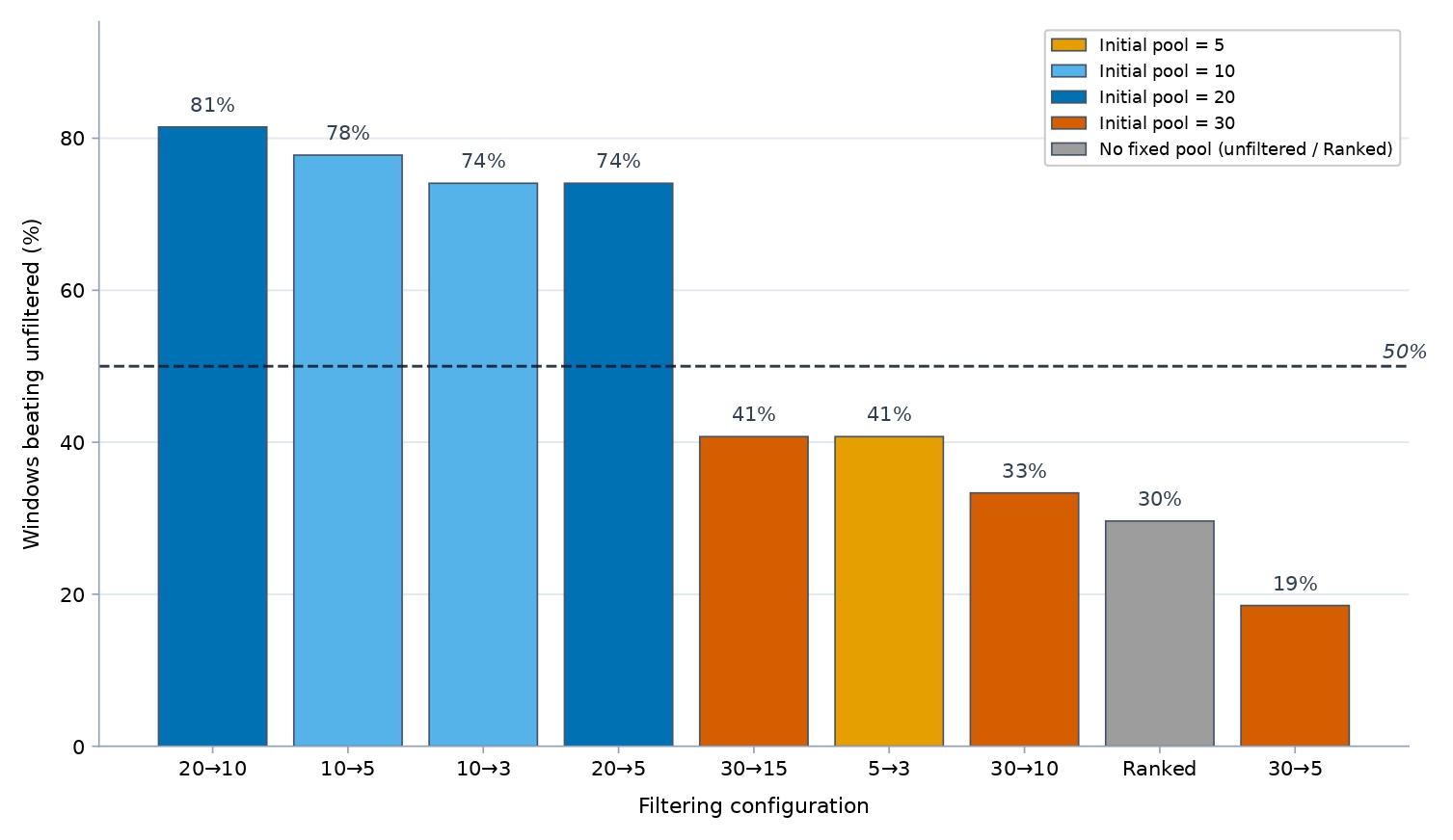
Filtering substantially improved GPT-5.1’s performance (Figure 2). 20→10 beat the unfiltered baseline in 81.5% of matched window comparisons (22/27; exact 95% CI [61.9, 93.7]), followed by 10→5 (77.8%; CI [57.7, 91.4]) and 10→3 and 20→5 (both 74.1%; CI [53.7, 88.9]). The exception was 5→3 (40.7%; CI [22.4, 61.2]), which trades return for the lowest run-to-run variability (see Return Variance and Consistency Comparison). The well-sized configurations thus beat single-pass prompting in roughly three of four matched window comparisons. These four configurations also performed much better in ROI than the unfiltered baseline: 20→10 achieved the highest mean ROI (60.6%), followed by 10→5 (56.2%), 10→3 (54.1%), and 20→5 (50.4%), all well above the baseline’s 45.7%.
When the initial pool was too large, performance dropped sharply. The three configurations that started with an oversized thirty-candidate Stage One pool and the Ranked configuration underperformed the unfiltered baseline (30→5: 32.3%, 30→10: 40.1%, 30→15: 44.2%, and Ranked: 38.9% vs unfiltered baseline: 45.7%). All ten configurations are interpreted together in the following analyses.
Configurations with an oversized initial pool did not reduce risk enough to offset their reduced ROI, with both ROI and risk-adjusted ROI being lower than other configurations (30→5 returns 32.3% at a median Sharpe of 1.30, against 60.6% at 1.70 for 20→10; Table 1). Mean ROI follows an inverted-U when looking at differences in initial pool size (and holding model and evaluation windows constant): 42% at five candidates, 55% at ten and twenty, and 39% at thirty. Therefore, return decreases when the initial pool size exits that mid-range. The likely reason for configurations with a higher initial pool underperforming was that after 10-20 candidates, the model begins outputting marginal stocks that it would not have otherwise produced due to the 30 stock requirement. These lower-potential stocks pollute the second stage of the filtering, leading to a poor final portfolio. Changing the size of filtering in the second stage did not close the gap between the thirty-candidate and mid-sized configurations, suggesting that the initial stage is more impactful on results. For lower initial-size configurations, the number of stocks is so low that the model isn’t able to retrieve enough stocks for a strong portfolio.
Based on these results, we can see that the organization of information strongly affected performance for GPT-5.1. An initial moderate pool of 10-20 candidates before going into Stage Two maximizes return, while lower sizes trade a large amount of return for higher stability and higher sizes drop return substantially for minimal risk decreases.
| Configuration | Mean ROI (%) | Volatility (%) | Max DD (%) | Sharpe | Win vs Unfiltered (%) | 95% CI (Win %) |
| 20→10 | 60.6 | 28.1 | −23.2 | 1.70 | 81.5 | [61.9, 93.7] |
| 10→5 | 56.2 | 26.6 | −23.6 | 1.61 | 77.8 | [57.7, 91.4] |
| 10→3 | 54.1 | 26.0 | −23.0 | 1.54 | 74.1 | [53.7, 88.9] |
| 20→5 | 50.4 | 27.0 | −24.2 | 1.55 | 74.1 | [53.7, 88.9] |
| unfiltered | 45.7 | 27.8 | −22.4 | 1.34 | — | — |
| 30→15 | 44.2 | 25.6 | −22.3 | 1.43 | 40.7 | [22.4, 61.2] |
| 5→3 | 42.2 | 24.9 | −22.6 | 1.43 | 40.7 | [22.4, 61.2] |
| 30→10 | 40.1 | 24.4 | −21.8 | 1.35 | 33.3 | [16.5, 54.0] |
| Ranked | 38.9 | 23.9 | −21.7 | 1.40 | 29.6 | [13.8, 50.2] |
| 30→5 | 32.3 | 22.4 | −21.6 | 1.30 | 18.5 | [6.3, 38.1] |
To determine whether the apparent advantage over the unfiltered baseline is from the sequential structure or simply due to the amount of material in the prompt being less, we conducted ablation tests. Keeping the candidate documents the same for GPT-5.1’s 20→10 configurations across all date windows (with 2-4 generations per condition), we compared the full pipeline (considered A2 in this case) against four different arms: a single prompt carrying data for the broader thirty-candidate pool (A1); a variant that shows the same twenty reports as the pipeline but selects the final portfolio with a differently worded single-step instruction (A3); a variant in which the financial summaries are shuffled across tickers while each company’s news rationale is kept (A4); and a single prompt carrying the same news and the same twenty shortlisted companies’ reports as the pipeline, so the two differ only in one call versus two (A5) (arm labels and token counts in Table S5a). The original full pipeline (A2) still produced higher mean ROI than any other arm (52.4%). It beat the A5 configuration by 5.0 percentage points in six out of nine windows (with a Wilcoxon p of 0.055) and A1 by 3.3 points in six out of nine windows (p = 0.25), while A3 trailed by 3.7 points (p = 0.570). Arms A2, A3, and A4 (sequential arms) are within 0.1% of token count, so the ROI drop from shuffling the reports is due to the content differing, not the length. The arms A1 and A5 (single-pass arms) have roughly double the number of tokens as the sequential arms (since they combine content for two arms into one), but it’s clear that token length is not what determined the difference in performance between the two, since A5 had less tokens but still was outperformed by A1 (47.2% against 49.0%). Once the window is controlled, prompt length also does not predict return (r = +0.03 across 204 arm-runs). Full paired statistics are in the Supplementary Information.
Formal paired statistics support these comparisons. For each configuration, the per-window ROI difference against the matched unfiltered baseline was evaluated with an exact sign test and a Wilcoxon signed-rank test, and computed a bootstrap 95% confidence interval on the median difference. On this 27-pair basis (which pairs replicate-group means and therefore overstates the independent information in the design), the four moderate configurations differ significantly from the baseline (20→10: sign-test p = 0.002, Wilcoxon p < 0.001; 10→5: p = 0.006; 10→3 and 20→5: p = 0.019), the mid-table configurations can not be statistically distinguished from it, and 30→5 is significantly worse (5/27 wins; p = 0.002). Because the 12-month windows overlap, these pairs should also be treated as matched comparisons rather than as results from separate independent years. At the window level (n = 9), obtained by collapsing GPT-5.1’s three replicate generations per window, 20→10 remains significant (8/9 wins; sign-test p = 0.039; Wilcoxon p = 0.027), 20→5 remains significant by the sign test (8/9 wins; p = 0.039; Wilcoxon p = 0.129), and 30→5 remains significantly negative (0/9 wins; p = 0.004), while 10→5 and 10→3 (7/9 wins each; sign-test p = 0.180; Wilcoxon p = 0.098) fall short of significance at that resolution. Window-level results for every configuration appear in the Supplementary Information, and per-configuration confidence intervals accompany every win rate in Table 1.
Overall Trends
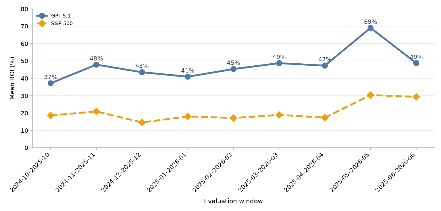
GPT-5.1’s mean ROI beats the S&P 500 in every window we tested, and it beat the index on a risk-adjusted basis too (median Sharpe 1.70 for 20→10 against 0.98 for the index over the same windows.) Figure 3 plots its mean ROI across each rolling 12-month window against the benchmark. Performance moved with the market but stayed above the benchmark the whole way. Across all GPT-5.1 runs, 604 of 626 (96.5%) beat the S&P 500 over their holding window. That counts every run however, not one per cell, so it is a fraction of 626, not part of the 270 window x generation group x configuration cells.
GPT-5.1 contributes nine completed rolling windows, with start dates from October 2024 through June 2025 (end dates October 2025 through June 2026). Earlier windows are excluded by the model’s training cutoff constraint. The weakest window, October 2024 to October 2025, still returned 37.1%. The strongest, May 2025 to May 2026, reached 69.0%. Both are well above the matching benchmark return.
The unfiltered baseline also beat the S&P 500 in every window. The market outperformance only reflects the model and sector strength, not the filtering itself. The filtering’s contribution shows up in the matched comparison against the baseline (see Filtered vs Unstructured Baseline), where the well-specified configurations win around roughly three of four windows. Benchmark returns ranged from 15% to 30%, while GPT-5.1 returned between 37% and 69%.
Return Variance and Consistency Comparison
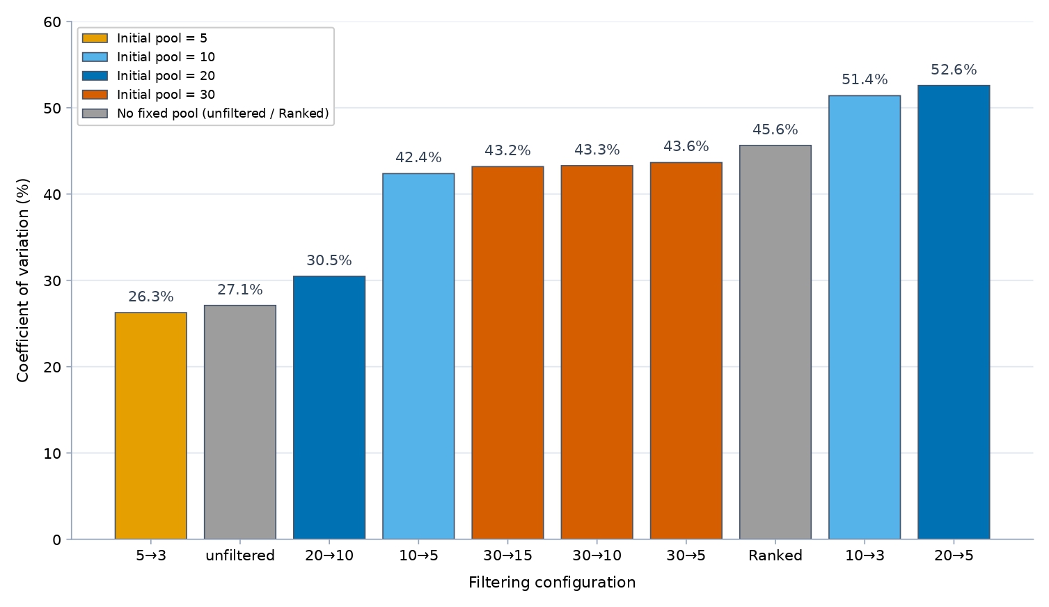
Filtering also affected how consistent returns were. Returns were the steadiest at both extremes of filtering, and had more variable in between. Figure 4 reports each configuration’s coefficient of variation (CV). Lower CV means returns cluster more tightly around the mean.
For GPT-5.1, the most consistent configurations were the highly selective 5→3 (CV 26.3%) and unfiltered baseline (27.1%) with 20→10 close behind (30.5%). The highest returning configurations (10→5, 20→5, and 10→3) were moderately less consistent (CV 42-53%). The higher returns came with a wider run-to-run spread.
This ordering follows from the same structural settings that drive return, not from chance. Run-to-run variability is lowest when the second stage is the most decisive relative to its input. Either the pool is small enough that the final choice is nearly forced (5→3), or no filtering is imposed at all (the unfiltered baseline).. It is highest for the mid-ratio configurations, which carry more borderline candidates into the final portfolio. Their stability and return are shaped by the same interaction, which is between the initial pool and the ratio. So the return-maximizing 20→10 ranks just below the most stable configurations instead of the most variable.
The configuration shapes the average level of return, but not the outcome of any runs. Within a given configuration, individual runs vary more than the configurations’ means they differ from one another. Most of that run-to-run variation traces to the evaluation window (the prevailing market regime) and to the model’s stochastic re-selection of stocks on each run, not the configuration itself. So we assess the configuration effect through averaged ROI and matched window-by-window win rates. Those hold the market regime fixed and let the systematic differences emerge, rather than relying on the spread of individual runs.
Filtering affects both the level of GPT-5.1 returns and their spread. A practitioner can give up some return for a more predictable approach. By moving toward the more selective end of the grid.
Model Comparison and Configuration Selection
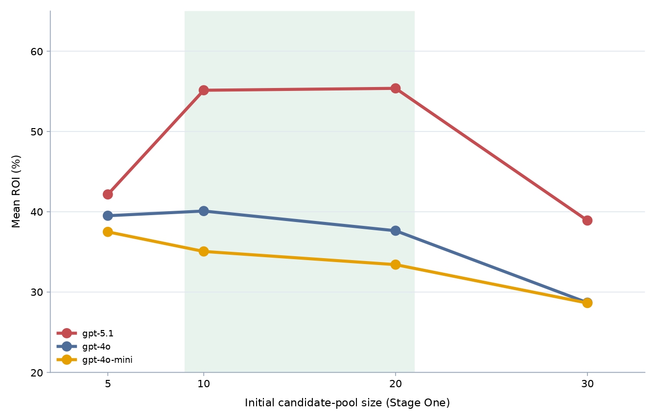
The underlying model and how the desired portfolio size maps onto the two stages are the two factors that determine which configuration to deploy. Figure 5 compares the three models across fixed-pool configurations. Table 1 and the matched win rates from Figure 2 identify the best configuration for each target portfolio size. Additionally, the unfiltered single-pass run is the baseline throughout.
In Figure 5, mean ROI is plotted against the initial candidate-pool size for each of the three models. GPT-5.1, which is shown in red, produced the highest ROI at every pool size. It averaged 47.0% across all of its runs (equivalently, an unweighted 46.5% across its ten per-configuration means, or also 47.5% across the eight fixed-pool configurations in Table 1). Run-level means were 35.0% for GPT-4o and 32.7% for GPT-4o-mini. This is a gap of roughly 12 to 14 percentage points, which holds across pool sizes. However, the shape of the curve differs by model. GPT-5.1 shows a pronounced inverted-U, which peaks at 10-20 candidates. GPT-4o peaks at only 10, and its five-candidate pool outperforms its twenty. Finally, GPT-4o-mini declines steadily from a maximum of five candidates. All three models have a penalty for using oversized pools, as shown by the fact that every model declines at thirty candidates. This pattern suggests that the optimal pool size scales with how capable the model is. A stronger model can fill a request with more candidates with confidence, but weaker models do best when they are asked for only as many names as they can justify. Raw model capability sets the overall return level, and the pipeline configuration determines how much of that level is actually realized.
The same data indicates how the best configuration shifts with the desired portfolio size (Table 1). For a three-stock portfolio, 10→3 is the best (54.1%). This beats the unfiltered baseline in 74.1% of matched windows and outperforms the more selective 5→3 (42.2%). For a five-stock portfolio, 10→5 leads (56.2%, and it beats the baseline 77.8% of the time). It is ahead of 20→5 (50.4%, 74.1%). For a ten-stock portfolio, 20→10 is the best option and the single highest-returning configuration in this study (60.6%). It beats the baseline in 81.5% of matched windows. From this, a consistent pattern emerges, which is that the best Stage One pool is roughly twice the target portfolio size. This is consistent with the 2× hypothesis. The over-filtered methods above are not recommended and are dominated at every portfolio size.
One further ablation asks if the report stage contributes company-specific content or just more structured text. Shuffling reports across tickers, each candidate is validated against another company’s financials. It produces the largest and only unambiguous decline, which is 9.3 percentage points below the full pipeline. It loses nine of nine windows (Wilcoxon p = 0.004). Therefore, the report-validation stage carries company-specific signals.
The configuration-by-target-size pattern remains for the same reason that was identified in the baseline comparison. A Stage One pool of around twice the target size gives the model enough candidates to rank. This does not overwhelm the validation stage. The amount of holdings desired helps determine which setup should be used. However, the main benefit comes from starting with a reasonable number of candidates and then narrowing the group down, not from any specific configuration.
Sector Allocation and Realized Returns
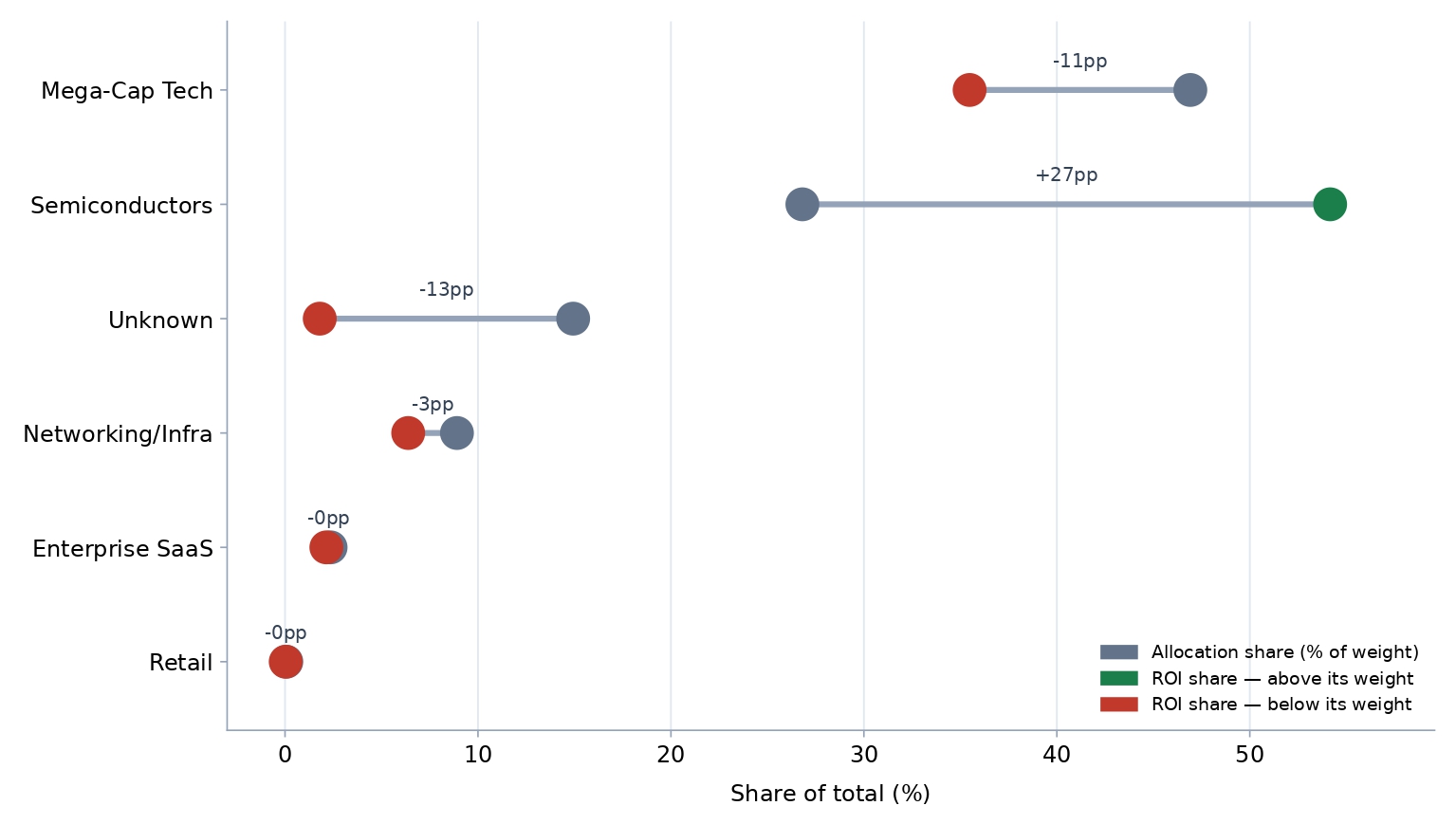
The sector composition of GPT-5.1’s portfolios shows where its performance originated beyond aggregate returns. Figure 6 compares each sector’s share of the recommended portfolio weight with the share of the realized return. GPT-5.1 allocated the largest share of capital to Mega-Cap Technology, and it was 46.9% of weight. However, that sector only delivered 35.5% of realized ROI. Semiconductors, which had 26.8% of the weight, contributed 54.2% of the realized return. This is roughly twice their allocation, making them the dominant source of performance. Networking/Infrastructure (8.9% of weight and 6.4% of ROI) and Enterprise SaaS (2.4% of weight and 2.1% of ROI) contributed close to their original proportions. A 14.9% allocation to unclassified holdings produced only 1.8% of realized returns. These results indicate that the framework’s returns were driven disproportionately by semiconductor selections, and allocation share by itself understates where performance actually originates. A sector’s share of realized returns is the sum across that sector’s holdings of each position’s initial weight times its window return, divided by the portfolio’s total return. Both quantities are pooled across runs. Averaging gives the same result because the per-run count cancels. Since individual contributions from a sector can be negative, the return share for a sector can exceed or fall below its weight share. The shares sum to 100% total.
Benchmark Robustness, Ablations, and Weighting
The S&P 500 comparison overstates selection performance because the eligible universe consists of technology and semiconductor companies that outperformed the broad market during the study period. Against comparable benchmarks, GPT-5.1’s overall win rate falls from 96.5% against the S&P 500 to 94.3% against the Information Technology Index, 39.6% against an equal-weighted portfolio of the eligible universe, and 32.2% against a pure-semiconductor index (SMH). SMH provides a more sector-specific comparison because it consists of semiconductor companies. The filtering configurations outperform these benchmarks in the runs, as the 20 to 10 configuration outperforms the equal-weighted universe in 81.4% of runs and SMH in 68.3% of runs. The 10 to 5 configuration does so in 64.8% and 60.0% and the unfiltered baseline only reaches 18.5% and 6.7% against the same benchmarks respectively. All of these results are combined across the entire run set. The eligible comparison set is a fixed list of 29 large-capitalization technology and semiconductor companies (Supplementary Information). It is used for the unfiltered baseline and as the source pool for the equal-weighted and random benchmarks. The filtered configurations do not receive this list and instead nominate candidates from the screened news. Every company in the set remained on the public market throughout the evaluation. Because the same 29 companies are used throughout the evaluation period, the benchmark is not needed to be rebuilt for each evaluation date. A limitation is that the companies that were large enough to qualify at the start but eventually no longer qualified, were excluded. The set holds companies whose prices declined substantially, so it is not just a collection of stocks that performed well. This limitation affects the construction of the benchmark instead of the operation of the filtering pipeline. To test selection skill, random portfolios are established from the eligible universe and matched to each portfolio’s holding count and equal-weighted. Relative to 4000 random draws per run, the median GPT-5.1 portfolio under 20 to 10 falls at the 75th percentile and the 10 to 5 configuration reaches the 69th percentile. In comparison, the unfiltered baseline is at the 40th percentile, while the aggressive 30-pool configurations are near the 17th to the 21st percentile. This shows that the moderate two stage filtering produces portfolios that perform above the random benchmark within the sector. Two sensitivity checks were used to test whether this advantage depends on specific holdings. Removing the single largest return contributor from every portfolio lowers GPT-5.1’s 20→10 mean ROI from 60.6% to 52.5% and the unfiltered baseline from 45.7% to 39.4%. As a result, the matched filtering advantage narrows only modestly, from about +14.9 to +13.1 percentage points. Excluding all semiconductor holdings and renormalizing the weights leaves a smaller advantage of +3.0 percentage points. Therefore, the filtering advantage does not depend on any single position, since it remains intact after removing each portfolio’s largest contributor. However, the smaller the advantage after removing the semiconductors shows that semiconductor selection contributes significantly to the overall difference. Finally, every portfolio was scored again using equal weights to separate stock selection from allocation weighting. For GPT-5.1, the model-assigned weights reduce the mean ROI by 4.6 percentage points compared with equal-weighting the same stocks (Wilcoxon p < 0.0001). GPT-4o shows a smaller reduction of 1.2 percentage points, while the difference for GPT-4o-mini is approximately 0. The results show that the selected stocks contribute more to returns than the model-assigned weights. The models’ selection adds value, while their position sizing reduces the returns. Sector-index returns, random-portfolio percentiles, ablation tables, and per-configuration risk metrics (annualized volatility, maximum drawdown, Sharpe, and Sortino ratios) are provided in the Supplementary Information. The risk adjusted results follow the same pattern as the raw returns. For GPT-5.1, the 20 to 10 configuration has a median Sharpe ratio of 1.70 and a median Sortino ratio of 2.66. The unfiltered baseline has corresponding values of 1.34 and 2.04, while the S&P 500 has a median Sharpe ratio of 0.98 over the same windows. The weakest configuration, 30 to 5, has a median Sharpe ratio of 1.30. Volatility remains relatively the same across the configurations, ranging from 22% to 28%. Maximum drawdowns also remain within a range of -21.6% to -24.2%. This shows that the higher returns from moderate filtering are not accompanied by proportionally larger increases in volatility or drawdown. Full volatility, drawdown, and risk-adjusted statistics for every configuration and model are reported in the Supplementary Information.
Discussion
Implications and Significance
The results show that the method by which the information was given to the model affected the stock it chose. The best results usually came from giving it a moderate group of stocks first and then narrowing the group down. This did better than either giving it a large list with less filtering or making it remove most of the stocks from a large group, so the improvement came from changing how the process worked, and is not impacted by the model size.
Starting with around ten to twenty stocks and then narrowing the list down worked best for stronger m models, but the weaker models did better when starting with fewer stocks, which may mean that there might not be a consistent starting list size for all models. Specifically for GPT-5.1, it had different results based on how many candidates it started with. Performance was better when the candidate pool was larger, but then it went back down. A small pool gave the model few choices, but a large pool made weaker final selections. There are limitations to this, as the study did not track if the weaker stocks in bigger groups were what directly resulted in lower returns. To find this out, in future work, the first list can be compared with the final list to see what stocks remained and whether their original position related to realized returns. However, this remains a hypothesis as the original candidate lists were not saved and could not be checked again.
The unfiltered baseline also outperformed the market benchmark, so the main finding from the two-stage approach is more than just beating the market. What mattered more is that it consistently did better than the unfiltered baseline under the same conditions being used. This makes it more likely that differences came from how the information was presented instead of just a different model.
Limitations and Future Work
Some factors limit these findings. All portfolios are long-only and use a buy-and-hold strategy. Returns do not include transaction costs, taxes, or slippage, which lower performance. The investment universe is limited to large-capitalization technology and semiconductor companies, so the result may not apply to broader markets. GPT-5.1 was only tested on windows that started after its training cutoff. Because of this, there were fewer rolling windows for GPT-5.1, starting in October 2024, than for the older models. All of the windows also took place during generally a rising market. Because of this, the performance of the method during a long market decline has not been tested. Ten configurations were tested to find the one with the highest mean ROI. The 20→10 configuration had the highest mean ROI, but the same windows were used to choose the configuration and report its results. Because of this, the reported 60.6% return may be higher than what would be seen on new data. A split-sample test helped check for this. When the first five windows were used to choose the configuration, the same 20→10 configuration was selected. The four remaining windows returned 71.40%, compared with 55.88% for the matched unfiltered baseline. This was a 15.52pp gain, with the filtering approach winning in three of the four tests. The matched-baseline win rate and its confidence interval are a more conservative way to summarize the results because they do not depend on choosing the best configuration after looking at the results. The financial report data also has some limits. The source does not flag restatements or amendments. A restated figure keeps the fiscal period end date from the original filing, so it is treated as public from that date even if the corrected value appeared later. Because of this, some report values may include information that was not actually available at the time. The news screening process also limits the amount of information used. Its estimated recall compared with human readings ranges from 26.2 to 41.0% after reweighting. All of the articles also come from one source, so the companies considered are based on only part of the relevant news. The high precision helps keep unrelated material out, but the effect of changing the screening threshold has not been tested yet.
Future work will address these limits by adding transaction costs, testing stocks outside of technology, and evaluating the method during bear markets as more post-cutoff data becomes available. Live testing on new data would provide a stronger test of whether the advantage over the unfiltered method continues to hold. This would also test the recommended configuration on new data instead of using windows that were already part of the historical evaluation.
Conclusion
This study was used to see if changing the way information was given to the model can improve the selection of stocks. The results showed that it could. Using news to narrow down a group of stocks and then checking them with financial reports worked better than giving the model all the information without filtering or filtering out too many stocks. There were a total of 2759 portfolio runs. The approach that worked best started with ten to twenty stocks and then broke the group in half. It had a mean ROI about fifteen percentage points higher than the unfiltered baseline, doing better in most of the time periods that were compared. The range is not a rule though, but worked best for what we tested. One of the main things from the study was that the way information is given to the model can make a difference. It was around as important as which model was being used. There are still limitations to the study so the results could be different if this was tested with other stocks, models, or time periods. Overall, the results suggest that what information the model gets and how it is given matters the most.
Data and Code Availability
To make the study reproducible, materials are publicly available at https://github.com/JathinBat/LLM-Two-Stage-Portfolio-Filtering. This included the prompts used for news screening, Stage One, Stage Two and the unfiltered and ranked baselines, along with all evaluation windows, the results from each run, including tickers, weights, and decision dates, and analysis scripts. The scripts also contain the paired-difference statistics, risk-metric calculations, and benchmark reconstruction. The news from The New York Times and financial reports from Alpha Vantage are not included because they cannot be redistributed under their terms. But the Methods and Supplementary Information explain the retrieval queries, date ranges, and timestamp rules used to collect the data, so the same datasets can be rebuilt using the documented process.
Supplementary Information
References
- Y. Nie, Y. Kong, X. Dong, J. M. Mulvey, H. V. Poor, Q. Wen, S. Zohren. A survey of large language models for financial applications: progress, prospects and challenges. arXiv, 2024, https://doi.org/10.48550/arXiv.2406.11903. [↩] [↩] [↩] [↩] [↩]
- S. An, Q. Li, J. Lu, D. Yin, X. Sun. FinVerse: an autonomous agent system for versatile financial analysis. arXiv, 2024, https://doi.org/10.48550/arXiv.2406.06379. [↩] [↩]
- A. Lopez-Lira, Y. Tang. Can ChatGPT forecast stock price movements? return predictability and large language models. SSRN. 2023, https://doi.org/10.2139/ssrn.4412788. [↩] [↩] [↩] [↩] [↩] [↩] [↩] [↩] [↩]
- Y. Xiao, E. Sun, D. Luo, W. Wang. TradingAgents: multi-agents LLM financial trading framework. arXiv, 2024, https://doi.org/10.48550/arXiv.2412.20138. [↩] [↩] [↩] [↩] [↩]
- H. Ding, Y. Li, J. Wang, H. Chen. Large language model agent in financial trading: a survey. arXiv, 2024, https://doi.org/10.48550/arXiv.2408.06361. [↩] [↩]
- W. W. Li, H. Kim, M. Cucuringu, T. Ma. Can LLM-based financial investing strategies outperform the market in the long run? arXiv, 2025, https://doi.org/10.48550/arXiv.2505.07078. [↩] [↩] [↩] [↩] [↩] [↩]
- D. Blitz, M. X. Hanauer, T. Hoogteijling, C. Howard. The term structure of machine learning alpha. The Journal of Financial Data Science. Vol. 5, pg. 40–65, 2023, https://doi.org/10.3905/jfds.2023.1.135. [↩]
- G. Lu, S. B. Larcher, T. Tran. Hybrid long document summarization using C2F-FAR and ChatGPT: a practical study. arXiv, 2023, https://doi.org/10.48550/arXiv.2306.01169. [↩]
- H. Naveed, A. U. Khan, S. Qiu, M. Saqib, S. Anwar, M. Usman, N. Akhtar, N. Barnes, A. Mian. A comprehensive overview of large language models. ACM Transactions on Intelligent Systems and Technology. Vol. 16, no. 5, 2025, https://doi.org/10.1145/3744746. [↩]
- B. Cao, S. Wang, X. Lin, X. Wu, H. Zhang, L. M. Ni, J. Guo. From deep learning to LLMs: a survey of AI in quantitative investment. arXiv, 2025, https://doi.org/10.48550/arXiv.2503.21422. [↩] [↩]
- I. Mirzadeh, K. Alizadeh, H. Shahrokhi, O. Tuzel, S. Bengio, M. Farajtabar. GSM-symbolic: understanding the limitations of mathematical reasoning in large language models. International Conference on Learning Representations (ICLR 2025). 2025, https://openreview.net/forum?id=AjXkRZIvjB. [↩] [↩] [↩]
- I. Okpala, A. Golgoon, A. R. Kannan. Agentic AI systems applied to tasks in financial services: modeling and model risk management crews. arXiv, 2025, https://doi.org/10.48550/arXiv.2502.05439. [↩]
- Y. Zhang, Y. Li, L. Cui, D. Cai, L. Liu, T. Fu, X. Huang, E. Zhao, Y. Zhang, C. Xu, Y. Chen, L. Wang, A. T. Luu, W. Bi, F. Shi, S. Shi. Siren’s song in the AI ocean: a survey on hallucination in large language models. Computational Linguistics. Vol. 51, pg. 1373–1418, 2025, https://doi.org/10.1162/coli.a.16. [↩] [↩] [↩] [↩]
- G. Fatouros, K. Metaxas, J. Soldatos, M. Karathanassis. MarketSenseAI 2.0: enhancing stock analysis through LLM agents. arXiv, 2025, https://doi.org/10.48550/arXiv.2502.00415. [↩] [↩] [↩] [↩] [↩]
- J. Cheng, P. Chin. AAPM: large language model agent-based asset pricing models. arXiv, 2024, https://doi.org/10.48550/arXiv.2409.17266. [↩]
- C. Choi, A. Lopez-Lira, Y. Lee, J. Kwon, M. Kim, J. Hwang, M. Ha, C. Kim, J. Ha, S. Yun, J. Kim. Structuring the unstructured: a multi-agent system for extracting and querying financial KPIs and guidance. arXiv, 2025, https://doi.org/10.48550/arXiv.2505.19197. [↩] [↩]
- T. Guo, X. Chen, Y. Wang, R. Chang, S. Pei, N. V. Chawla, O. Wiest, X. Zhang. Large language model based multi-agents: a survey of progress and challenges. Proceedings of the 33rd International Joint Conference on Artificial Intelligence (IJCAI 2024), Survey Track. 2024, https://doi.org/10.24963/ijcai.2024/890. [↩] [↩]
- X. Han, N. Wang, S. Che, H. Yang, K. Zhang, S. X. Xu. Enhancing investment analysis: optimizing AI-agent collaboration in financial research. Proceedings of the 5th ACM International Conference on AI in Finance. 2024, https://doi.org/10.1145/3677052.3698645. [↩] [↩]
- C. Zhang, X. Liu, M. Jin, Z. Zhang, L. Li, Z. Wang, W. Hua, D. Shu, S. Zhu, X. Jin, S. Li, M. Du, Y. Zhang. When AI meets finance (StockAgent): large language model-based stock trading in simulated real-world environments. arXiv, 2024, https://doi.org/10.48550/arXiv.2407.18957. [↩] [↩] [↩]
- Y. Li, Y. Yu, H. Li, Z. Chen, K. Khashanah. TradingGPT: multi-agent system with layered memory and distinct characters for enhanced financial trading performance. arXiv, 2023, https://doi.org/10.48550/arXiv.2309.03736. [↩]
- Y. Yu, H. Li, Z. Chen, Y. Jiang, Y. Li, D. Zhang, R. Liu, J. W. Suchow, K. Khashanah. FinMem: a performance-enhanced LLM trading agent with layered memory and character design. Proceedings of the AAAI Symposium Series. Vol. 3, pg. 595–597, 2024, https://doi.org/10.1609/aaaiss.v3i1.31290. [↩] [↩] [↩]
- T. Guo, H. Shen, J. Huang, Z. Mao, J. Luo, B. Chen, Z. Chen, L. Liu, B. Xia, X. Liu, Y. Ma, M. Zhang. MASS: multi-agent simulation scaling for portfolio construction. arXiv, 2025, https://doi.org/10.48550/arXiv.2505.10278. [↩]
- J. Li, J. Zhang, H. Li, Y. Shen. An agent framework for real-time financial information searching with large language models. arXiv, 2025, https://doi.org/10.48550/arXiv.2502.15684. [↩] [↩]
- K. Chen, H. Ahmad, D. Goel, C. Szabo. 3S-trader: a multi-LLM framework for adaptive stock scoring, strategy, and selection in portfolio optimization. arXiv, 2025, https://doi.org/10.48550/arXiv.2510.17393. [↩]
- T. Zhao, J. Lyu, S. Jones, H. Garber, S. Pasquali, D. Mehta. AlphaAgents: large language model-based multi-agents for equity portfolio constructions. arXiv, 2025, https://doi.org/10.48550/arXiv.2508.11152. [↩]
- T. Zhou, P. Wang, Y. Wu, H. Yang. FinRobot: AI agent for equity research and valuation with large language models. arXiv, 2024, https://doi.org/10.48550/arXiv.2411.08804. [↩]
- W. Zhang, L. Zhao, H. Xia, S. Sun, J. Sun, M. Qin, X. Li, Y. Zhao, Y. Zhao, X. Cai, L. Zheng, X. Wang, B. An. A multimodal foundation agent for financial trading: tool-augmented, diversified, and generalist. Proceedings of the 30th ACM SIGKDD Conference on Knowledge Discovery and Data Mining. 2024, https://doi.org/10.1145/3637528.3671801. [↩]
- P. C. Tetlock. Giving content to investor sentiment: the role of media in the stock market. The Journal of Finance. Vol. 62, pg. 1139–1168, 2007, https://doi.org/10.1111/j.1540-6261.2007.01232.x. [↩] [↩] [↩]
- J. Lee, N. Stevens, S. C. Han, M. Song. A survey of large language models in finance (FinLLMs). Neural Computing and Applications. Vol. 37, pg. 24853–24867, 2025, https://doi.org/10.1007/s00521-024-10495-6. [↩] [↩] [↩]
- S. Wang, H. Yuan, L. M. Ni, J. Guo. QuantAgent: seeking holy grail in trading by self-improving large language model. arXiv, 2024, https://doi.org/10.48550/arXiv.2402.03755. [↩] [↩] [↩]
- K. Anjum, M. A. Arshad, K. Hayawi, E. Polyzos, A. Tariq, M. A. Serhani, L. Batool, B. Lund, N. R. Mannuru, R. V. K. Bevara, T. Mahbub, M. Z. Akram, S. Shahriar. Domain specific benchmarks for evaluating multimodal large language models. arXiv, 2025, https://doi.org/10.48550/arXiv.2506.12958. [↩]
- H. Li, Y. Cao, Y. Yu, S. R. Javaji, Z. Deng, Y. He, Y. Jiang, Z. Zhu, K. Subbalakshmi, G. Xiong, J. Huang, L. Qian, X. Peng, Q. Xie, J. W. Suchow. InvestorBench: a benchmark for financial decision-making tasks with LLM-based agents. Proceedings of the 63rd Annual Meeting of the Association for Computational Linguistics (ACL 2025). pg. 2509–2525, 2025, https://doi.org/10.18653/v1/2025.acl-long.126. [↩] [↩] [↩] [↩]