Predicting Effective Heuristics and Optimality Gap for the Traveling Salesman Problem Using Lightweight Instance Features

Abstract

The Traveling Salesman Problem (TSP) seeks the shortest Hamiltonian cycle in a graph. Because it is NP-hard, solutions for large instances must be approximated with heuristics whose performance varies by instance. We present a two-stage pipeline predicting the best-performing heuristic and its optimality gap respectively from nine cheap structural features without running any heuristic in advance. It is trained on 160 instances (Euclidean, Geo, and synthetically generated Explicit) across Nearest Neighbor, Greedy, Christofides, and Insertion heuristics. Within the pipeline, Stage 1 utilizes Logistic Regression, Random Forest, and XGBoost, while Stage 2 runs a gap regressor with Quantile Regression or Conformal Prediction intervals, with features normalized to dimensionless ratios to maintain scale invariance. Among the results, Random Forest attains 80.00%5.08% cross-validation accuracy with a mean regret of 0.028, a 66-fold reduction versus an always-Christofides baseline. Random Forest with Quantile Regression further achieves a gap MAE (Mean Absolute Error) of 5.21pp with 90.63% coverage on a fixed split, and performs best on 26 of 30 partitions in a repeated hold-out over thirty seeds, with MAE 29.5226.01pp and log-space R2 (0.8000.082). However, paired significance testing, corrected for overlapping resampled test sets, finds this advantage directionally consistent but not statistically significant, where both conformal variants achieve coverage indistinguishable from nominal, a limitation to concluding a single-best model. Among the tested features, triangle-inequality violation rate, violation magnitude, and normalized minimum spanning tree (MST) weight are the most influential. Finally, justifying our research premise of using features to predict the best heuristic, we find feature extraction plus inference to be 15.9 cheaper on average than running all four heuristics, rising to 62.7 on the largest instances.

Keywords: Traveling Salesman Problem, heuristic selection, algorithm selection, optimality gap, random forest, XGBoost, quantile regression, conformal prediction, combinatorial optimization, instance features.

Introduction

The Problem

The Traveling Salesman Problem (TSP) asks for the shortest Hamiltonian cycle in a graph. Tracing back to the 1800s, the initial roots of TSP can be attributed to Irish mathematician Sir William Rowan Hamilton, who introduced the icosian calculus¹, seeking a closed cycle which visits each vertex of a dodecahedron exactly once. This Hamiltonian circuit problem was placed by Karp² among the first twenty-one proven NP-complete problems, and accordingly, there is also no known polynomial-time optimal algorithm for TSP. Like other NP-Complete problems, the number of candidate tours grows factorially as the size of the problem increases. Hence, heuristics are used to approximate solutions instead.

However, heuristics possess their own problems. First, it is difficult to determine the optimality gap without access to the true optimal solution: although some algorithms such as Christofides guarantee an approximation factor of 1.5 for metric TSPs, most do not have such a definite interval. This is important, because the optimality gap prediction is a main factor behind assessing a heuristic-generated tour. Second, no single heuristic is uniformly best: empirical findings from the algorithm-selection literature³ demonstrate the idea of performance complementarity, where the no-free-lunch theorems formally state that no search algorithm dominates another when averaged over all objective functions⁴; hence, the most suitable one is dependent on various features of the problem, such as problem type and size to name a few. Third, the runtimes of heuristics can still become significant, ranging from at least O(n2) for Nearest Neighbor and Greedy to O(n3) for Christofides and Insertion. Therefore, despite their faster speed compared to a brute-force optimal solver, selecting the best heuristic under a short time budget is still highly relevant.

Current Landscape

The algorithm selection problem was formally defined by Rice⁵, whose model maps a problem space through a feature space onto an algorithm space followed by algorithm selection based on maximising a performance measure. This is the precise framework of our paper. It has since been applied across combinatorial domains: SATzilla⁶ used empirical hardness models over instance features to choose among constituent SAT solvers, winning three gold, one silver, and one bronze medal at the 2007 SAT Competition. Smith-Miles and Muñoz⁷ project instances into a two-dimensional space to identify regions of solver strength and weakness; Kotthoff⁸ surveys the methods used, and so on. Closer to the present work, Mersmann et al.⁹ built features from minimum spanning trees, nearest-neighbor distances, and convex hulls to separate Euclidean instances that 2-opt approximates well from those it does not, and Hutter et al.¹⁰ predicted solver runtime on SAT, mixed-integer programming (MIP), and TSP benchmarks through regression over instance features. Both predict performance from features, as we do. However, our framework proposed differs in two respects. First, it restricts itself to features computable in O(n2) or better (using sampling in certain cases to reduce runtime) and directly demonstrates they are cheap relative to the heuristics they replace, whereas prior feature sets were not constrained by extraction cost. Second, its predictions are presented within a calibrated prediction interval rather than as a point estimate alone, so that a practitioner receives an uncertainty alongside the recommended heuristic.

Project Overview

In this project, we explore to what extent it is possible to use simple, cost-effective computable features of a Traveling Salesman Problem instance to predict the optimal heuristic for a given problem and to predict the optimality gap, comparing three heuristic selectors and four end-to-end prediction pipelines. By TSP features, we refer to the number of cities, edge weights, minimum spanning tree weight, etc.; a total of nine features in this investigation. This matters because TSP optimization is used in delivery and logistics (e.g. Amazon, FedEx), ride-hailing and fleet dispatching, and printed-circuit-board drilling, applications that require quick routing decisions, whereas exact solvers such as Concorde and CPLEX can take hours or days on large instances: Hoos and Stützle measured a median Concorde running time of 344,131 seconds — nearly four days — on uniform random Euclidean instances of 4500 cities, and only 65 of the 100 such instances were solved at all¹¹. Throughout this paper, “best” or “optimal” heuristic refers only to the best-performing heuristic among the four tour-construction heuristics evaluated here (Nearest Neighbor, Greedy, Christofides, and Cheapest Insertion); modern local-search and metaheuristic methods (Lin–Kernighan–Helsgaun, 2-opt, 3-opt, Guided Local Search, Simulated Annealing, Genetic Algorithms, Ant Colony Optimization) fall outside this pool and are not compared against. Abbreviations used throughout are expanded at first use and collected in Table S1 of the supplementary material.

Methods

Different Heuristics

Tour-construction heuristics generate solution tours and tour-improvement heuristics refine them. Within the scope of this paper, we only focus on four tour-construction heuristics as summarized in Table 1. Rosenkrantz et al.¹² establish a bound for two of them on metric instances, where nearest and cheapest insertion never exceed twice the optimum and Nearest Neighbor can exceed it by a factor growing as . The metric condition for this bound is also what motivates us to measure violations of the triangle inequality among the features below..

Heuristic	Description	Runtime
Nearest Neighbor	Starts at a city and repeatedly moves to the closest unvisited neighbor. Averages roughly 25% above the Held–Karp bound on random uniform instances13.	O(n2)​
Greedy	Sorts all O(n2) edges globally and greedily adds the shortest edge that does not create a sub-cycle or exceed degree two at any city.	O(n2logn)​
Christofides	Builds an MST (minimum spanning tree), adds minimum-weight perfect matching on odd-degree vertices, then shortcuts an Eulerian circuit. Guarantees a tour within 1.5 optimal for metric instances14; the factor was later reduced to 1.5− for a small >015.	O(n3)​
Insertion (Cheapest)	Initializes a small subtour and repeatedly inserts the unvisited city at the position minimizing the increase in tour length.	O(n3)​

Obtaining Problems

We obtained the majority of TSP instances from TSPLIB¹⁶ at the mastqe/tsplib GitHub mirror, a collection of traveling salesman problem datasets maintained by Gerhard Reinelt. It contains mostly symmetric Euclidean 2D problems, with the original collection comprising 79 Euclidean_2D instances (distances derived from coordinates), 16 Explicit instances (distances provided in a complete matrix), and 10 Geo instances (distances account for the Earth’s curvature), 105 in total.

As observable, this dataset is mostly dominated by Euclidean_2D instances, a skew which risks biasing the learning model toward heuristics that perform well on metric, geometric inputs, most notably Christofides’ algorithm. To mitigate this bias and increase structural diversity, we generated 55 additional Explicit TSP instances which need not adhere to the triangle inequality. Although we acknowledge that these instances may not reflect real-world distributions, they serve to take the model beyond a biased, “Christofides-only” baseline, and expand the scope to include triangle inequality features, which aligns with the paper’s investigative purpose that aims to explore the relationship between different features and trends across instance types. The final result is a dataset of 79 Euclidean_2D instances, 71 Explicit instances, and 10 Geo instances, comprising a total of 160 problems.

The generated Explicit instances span three categories: Random instances that have symmetric distance matrices, independently sampled edge weights, and variable edge costs, serving as a baseline; Clustered instances, where vertices are partitioned into clusters with low-cost edges within them and high-cost edges connecting them, which prevents reliance on Euclidean geometry; and Christofides-hard instances, where the MST is misguided with low-cost edges to form an incorrect structural backbone. All instances are generated offline using deterministic procedures, enforced to be symmetric with zero diagonal entries, and exported in TSPLIB Explicit format.

Implementation of Heuristics

The four tour-construction heuristics of Table 1, including Nearest Neighbor (NN), Greedy, Insertion, and Christofides (CH), are implemented in Python, with the runtime of each on each instance recorded. Within 640 rows of the dataset, we excluded 23 entries due to them possessing a higher runtime than 600,000 ms, our hard runtime limit. However, seven of those still record a finished tour, so the Stage 2 gap table retains 624 rows rather than 617.

Features & Dataframe

We computed and recorded nine distinct, cheap properties for each of the 160 TSP instances, which serve as input parameters for the heuristic selection model (summarized in Table 2). Features that require long runtimes are estimated with Monte Carlo sampling to maintain feature cheapness.

Feature	Description	Complexity
type	Underlying distance model (Euclidean 2D, Geo, or Explicit); primarily differentiates metricity, i.e. if symmetry and the triangle inequality are expected to hold. The only categorical feature.	O(1)​
n	The number of cities; affects both the feasibility and runtime of heuristics.	O(1)​
min_edge_weight	The smallest non-zero edge weight, normalized by the instance’s mean edge weight; identifies closely connected node pairs, favoring local heuristics such as Greedy and Nearest Neighbor.	O(n2)​
cv_edge_weight	The coefficient of variation (standard deviation over mean); scale-free dispersion, comparable across instances.	O(n2)​
edge_weight_skewness	Asymmetry of the edge-weight distribution; a positive value indicates many short edges with a few very long ones, hence potentially damaging to greedy heuristics.	O(n2)​
pct_short_edges	The fraction of edges at or below the within-instance 10th percentile of edge weight, . Because the threshold is a within-instance percentile, this is pinned near 0.10 by construction and varies only through ties.	O(n2logn)​
triangle_violation_rate	The fraction of sampled node triples failing the triangle inequality; quantifies deviation from metric structure, which degrades Christofides. Monte Carlo estimate from 200,000 triples.	O(S)​
avg_violation_magnitude	The average severity of triangle-inequality violations, divided by the instance’s mean edge weight; larger values indicate stronger non-metric behavior.	O(S)​
mst_weight	Minimum spanning tree weight, normalized over nmean_edge_weight; a lower-bound proxy for tour length, directly relevant to Christofides.	O(n2)​

Since there are varying units across instances, and rescaling the edge weights of a TSP instance by a positive constant k does not change the optimal heuristic nor the percentage optimality gap of any tour, we expressed the numeric features as dimensionless ratios. Specifically, min_edge_weight and avg_violation_magnitude are each divided by the instance’s mean edge weight; mst_weight is normalized by nmean_edge_weight; and cv_edge_weight, edge_weight_skewness, triangle_violation_rate, and pct_short_edges are dimensionless by construction. Through this process, we also realized the redundancy of a candidate feature, std_edge_weight, since dividing it by the mean edge weight yields nothing but cv_edge_weight; we therefore dropped the former as a methodological improvement. To verify that the rescaled results are truly invariant, refer to the Results below. Ultimately, the feature set used throughout the rest of this paper is the nine features of Table 2: eight numeric features plus type.

For the Optimality Gap prediction model, we add an additional feature of heuristic during training, totaling ten features instead of nine. Hence, after one-hot encoding of heuristic and type, the actual number of feature labels is 11 for the heuristic selector model and 15 for the optimality gap model.

Throughout the investigation, all generalizations should be restricted to these features.

Heuristic Selector Model

An optimal heuristic is assigned to each instance based on a runtime constraint, which equals 600,000 ms; a heuristic is considered acceptable in case of meeting the runtime constraint; thus, runtime is taken into account while choosing a heuristic. Hence, the feasible best cost is:

   

where stands for the set of acceptable heuristics.

Split of 80/20 into training and testing sets has been done; it has been done by splitting instances instead of splitting rows to avoid leaking of information between train and test sets.

Class weighting has not been used since, for the majority of Euclidean_2D instances, Christofides is better than the others, while Nearest Neighbor has only 8 positive samples, and, hence, artificially up-weighting the minority classes would decrease the performance of the model.

As for models, there were three models considered at Stage 1. First of all, there was Logistic Regression with L2 regularization (C=1.0), using the L-BFGS solver as a baseline model; second, there was a Random Forest¹⁷ that has 400 trees, there is no maximum depth, as well as minimal number of samples per leaf is equal to 2. The third model is XGBoost¹⁸, which is a gradient-boosting with multi:softprob objective, 100 boosting rounds, maximum depth 3, learning rate =0.05, 80% subsample of instances and features for each tree, L2 regularization (=1.0). The LabelEncoder has been fitted on all class labels before running the cross-validation loop to minimize risks of class indexing mismatch in the pipeline.

All of the three models were assessed using a stratified 5-fold cross-validation (shuffle=True, random_state=1) with keeping distribution of classes in each fold (Christofides 46.9%, Insertion 28.8%, Greedy 19.4%, Nearest Neighbor 5.0%). Numerical features have been standardized, and type of instance has been one-hot encoded in a Pipeline to prevent leakage between folds. Afterward, each of the models was fitted on the whole set of data to determine influence of features. This way, a per-class coefficient matrix is received for the logistic regression model, and Gini-impurity importance and permutation importance (performed over 30 repeats) for the two other models. Performance of models is assessed using exact heuristic matching ratio, mean and median regrets, and catastrophic failure rate (regret >1).

Optimality Gap Model

Definition of Optimality Gap

The optimality gap is defined as the relative deviation of a heuristic solution from the true optimal tour length:

   

Predicting the optimality gap approximates the expected performance of a heuristic given a fixed instance without running it, precisely our research aim. It also adds nuance where several heuristics have similar costs: heuristic selection alone could rank one heuristic as the best and the other as a failure despite a marginal difference in their actual results, whereas a predicted gap would illustrate the degree of difference between different heuristic results.

Processing Data

We used the Concorde TSP Solver¹⁹ to compute optimal tours for most instances in the main dataset. For instances that Concorde cannot resolve within a reasonable time budget, the LKH implementation of the Lin–Kernighan heuristic²⁰ is used. Noting the heavily right-skewed gap distribution in the data (ranging from near 0% to over 5000% for Christofides’ application on certain Explicit instances), we applied a log transformation

   

to stabilize the variance and therefore improve model fit.

We train the gap predictor on the previous nine instance features but with the addition of a categorical indicator for the heuristic (Nearest Neighbor, Greedy, Insertion, Christofides), since the optimality gap model has access to predicted best heuristics from the heuristic selector, unlike the heuristic selector itself. To prevent data leakage, a fixed 80/20 train–test split and random seed is shared across both stages.

There is one mathematical consideration. Because ex is convex, back-transforming log-scale predictions via g=ey−1 underestimates the true conditional mean by Jensen’s inequality. Due to this and the approximate symmetry of log(1+g), we interpret the back-transformed prediction as an estimate of the conditional median gap.

Model

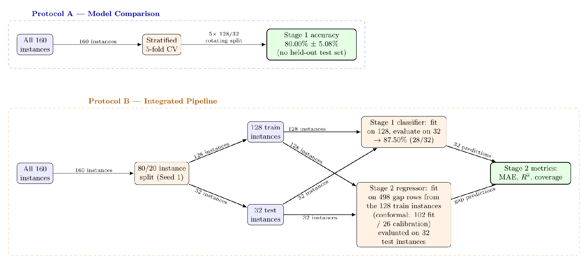
The optimality gap prediction pipeline contains two sequential stages, both trained on a shared 80/20 file-based split of the 160 instances, as set out in Figure 1. In Stage 1 a heuristic selector classifier is trained on the 128 training instances; at inference the heuristic label it selects is passed to Stage 2 as a tenth feature. Stage 1’s prediction errors therefore propagate into Stage 2, which is intended: the two stages are deployed together, and the error-propagation analysis below quantifies the effect.

Quantile Regression directly models the conditional quantiles of the response distribution; for the Random Forest backbone we use quantile regression forests²¹, which uses training responses in each leaf to estimate the full conditional distribution. Three regressors are trained at q=0.05,0.50,0.95, giving a lower bound, point estimate, and upper bound, so interval length adapts to instance difficulty; there is, however, no coverage guarantee, since empirical coverage depends on the training distribution representing the test distribution.

We therefore also employed Split Conformal Prediction²², whose split-sample form guarantees marginal coverage of at least 1− in finite samples under exchangeability of calibration and test data alone, with no assumption on the data distribution or the fitted regressor²³, at the cost of intervals that are symmetric in log space and uniform across instances rather than adaptive.

One important methodological consideration is the row calibration of instances. Because each TSP instance contributes four rows to the Stage 2 table, a row-level calibration split can place one heuristic row of an instance in the regressor’s training set and another row of the same instance in calibration, even though the two are not exchangeable. We therefore calibrate at the level of whole instances through a grouped shuffle split keyed on the instance identifier: of the 128 training instances, 102 fit the gap regressor and 26 are held out for calibration. The effective independent sample size for Stage 2 is accordingly at most 128 instances instead of the several hundred rows in the raw dataset.

To evaluate performance, we use integrated MAE (Mean Absolute Error), log-space R2 (coefficient of determination), empirical coverage, and interval width on the 32 held-out test instances.

Evaluation Protocol

We report two evaluation protocols, A and B. Protocol A cross-validates each Stage 1 selector over the full dataset with no held-out test set; since cross-validation uses every instance for both fitting and evaluation, the second stage is left with no data. We therefore introduce Protocol B, a single train/test instance split (with 30-seed repeated hold-out) that evaluates the complete two-stage pipeline and is the protocol behind every integrated pipeline result. Figure 1 shows the data flow for both, with all values verified (experiments/pipeline_provenance.py).

Results

Heuristic Selector

This subsection presents the Protocol A results, i.e. the model’s Stage 1 performance. We have incorporated stratified 5-fold cross-validation over all 160 instances with aggregated out-of-fold predictions. Before analysing the results, we first establish two performance baselines.

The first baseline, the Single Best Solver, always selects Christofides, since it is the most frequently optimal heuristic across the 160 instances (75 instances, 46.88%). Accordingly, this baseline yields an accuracy of 46.88%.

The second baseline, the Type-Based Rule, adopts a more flexible assigning rule of choosing Christofides for Euclidean_2D and Geo instances, and Insertion for Explicit instances. This rule achieves an elevated 68.13% accuracy.

It is clear that any useful model must exceed these baselines, and in accuracy they do, according to Table 3. We discuss each model individually in the remainder of this section.

Model	CV Accuracy	Train Acc.	Mean Regret	Catastrophic
Single Best Solver	46.88%	—	1.849	23.68%
Type-based rule	68.13%	—	0.074	0.66%
Logistic Regression	80.00% ± 7.02%	83.91%	0.119	1.25%
Random Forest	80.00% ± 5.08%	92.34%	0.028	0.63%
XGBoost	79.38% ± 6.12%	97.34%	0.029	0.63%

Logistic Regression

Across the stratified 5-fold cross-validation, logistic regression achieves accuracy in the region of 80.00%7.02%. This beats the Type-Based rule baseline, although its lower bound is barely above the same. Although an improvement, the limitations of the model render it as more of an improved baseline than an acceptable model. An example to illustrate this is the model’s predictions for the instance brg180, where the model predicts Greedy (cost 37,830) rather than Insertion (cost 2,420), producing a regret of 14.63. Analyzing the instance reveals that this is due to a moderately low triangle violation rate of 0.166 contrasted with a large normalized violation magnitude of 0.916, meaning the average triangle-inequality violation is nearly as large as an entire typical edge, which causes the boundary to misclassify. Such misclassifications are common for this model, as expected of a linear boundary’s performance in a classification model that is not trivially linear.

According to the mean absolute standardized coefficient across classes, logistic regression’s most influential features are cv_edge_weight (0.678), avg_violation_magnitude (0.595), and n (0.541). We omit a separate figure for this weaker baseline in this paper as part of the supplementary material, as the model is treated as a baseline and possess no extension in Stage 2, thereby holding less relevance for our results.

Random Forest

Across the 160 instances, the Random Forest classifier attains a cross-validation (CV) accuracy of 80.00%5.08% (via stratified 5-fold cross-validation), and a train accuracy of 92.34%. This CV figure exceeds the type-based rule by approximately 12 percentage points, which confirms that instance features can make a difference in guiding heuristic selection.

Per-class performance from the aggregated out-of-fold predictions can be found in Table S2 of the supplementary material. Bearing in mind Christofides’ dominance in label distribution (optimal for 75 of 160 instances), it is recovered reliably (precision 0.81, recall 0.91, F1 0.86), as is Insertion (46 instances; F1 0.83). However, Greedy (31 instances) is recovered less often (recall 0.65, F1 0.70), and Nearest Neighbor (8 instances) is effectively unlearnable due to its sample size, with precision, recall, and F1 of exactly 0.00 on this class (as is the case for the other two selectors). The full confusion matrix is given as Table S3 of the supplementary material.

Analysing the feature weights, Gini importance ranks the two triangle-inequality features highest (Table 4). Together these measure how severely the triangle inequality is violated, which directly affects the validity of Christofides’ approximation guarantee (factor 1.5 of optimal). We interpret the strong contribution of mst_weight as reflecting the relation between MST and greedy algorithms, where cheap spanning trees tend to be well-structured for greedy construction, as well as Christofides’ application of MST in its algorithm. These results do not deviate from our theoretical expectations. Permutation importance, however, places n first, which is justifiable considering that problem size governs the cost efficiency of heavy-weight heuristics, an important factor in heuristic selection; the reason the two rankings disagree is itself informative, and we return to it below.

Finally, when the model fails to predict the best heuristic it still often predicts a moderately good option. Indeed, the mean regret averaged over all scored instances is 0.0281 (considering the correct instance predictions contributing 0) and 0.144 if restricted to only the 31 misclassified instances. This is modest next to the 1.849 mean regret of always guessing Christofides in the first baseline. Furthermore, the regret value is also pulled up by rare outliers, as the catastrophic failure rate of 0.63% indicates. For example, christofides_hard_n50_s0 alone produces a regret of 3.168. Therefore, the actual regret for many incorrect instance predictions is even lower. We also note that regret is undefined if the predicted label does not record feasible heuristic costs, hence regret is not always calculated over all 160 instances: the denominator is 159 for both Random Forest and XGBoost, giving exact-match rates of 128/159=80.50% and 127/159=79.87%, and the full 160 for Logistic Regression, giving 128/160=80.00%.

Looking at the four costliest selections (excluding the costliest outlier above), they carry regret between 0.082 and 0.149, which is close to the 0.144 conditional mean. The most common error is when Christofides is predicted in the place of Greedy, happening nine times, although the gap between the two optimalities is marginal, corroborating our claim. Overall, most misclassifications occur between heuristics of comparable costs, making most selections still useful. Refer to Table S4 of the supplementary material for more detailed data about the classified instances, their predicted heuristic, true best heuristic, and regret.

XGBoost

XGBoost classifier configuration includes a maximum tree depth of 3 and 100 boosting rounds; in contrast, Random Forest utilizes the unoptimized default settings of 400 trees and no maximum depth. Taking the above-described difference into account, we conducted hyperparameter sensitivity analysis, where both of the described classifiers swept the grid of values for depth and number of rounds/trees (Tables S7, S8). The difference in sensitivity of the models is noticeable: while the accuracy of XGBoost varies by 5.01 percentage points (75.62% to 80.63%), Random Forest is in the range of 1.25 percentage points (78.75% to 80.00%).

Despite the above-mentioned sensitivity, the optimized configuration of XGBoost is valuable: only one of twenty grid cells exceeds its performance with 1.25 percentage points, which is small relative to the standard deviation of this grid (4.5–6%). Thus, even with a need for tuning, the comprehensive search is unlikely to discover significantly superior configuration compared with the optimized configuration discovered manually.

For the tuned model, the cross-validation accuracy is 79.38%6.12%, the training accuracy is 97.34%, resulting in train–CV gap of 18 percentage points. Distribution of per-fold accuracy is [0.9062,0.7812,0.7188,0.7812,0.7812]. From the instances with defined regret of 159 instances, the exact match rate is 127/159=0.7987. The mean regret is 0.0290, catastrophic failure rate is 0.63%, similar to Random Forest.

The XGBoost Gini feature importance (Table 4) is similar to Random Forest feature importance. The violation of triangle inequality (triangle_violation_rate, 0.215) is leading and more weighted than in Random Forest. At the same time, XGBoost differs from Random Forest in its second most important feature with weight 0.165 assigned to the feature called type_Explicit, before avg_violation_magnitude (weight 0.158).

We identified the high priority of type_Explicit as a possible risk. The classifier might depend on an arbitrary generator label rather than numeric properties of the instance in order to classify the instance. In order to examine this issue, we conducted an ablation, which revealed that removing the type feature does not affect cross-validation accuracy in two decimal points (79.38% for XGBoost and 80.00% for Random Forest, with difference of 0.00 points). This result indicates that the classifier is not dependent on “Explicit” label. Moreover, some of remaining numeric features correlate with provenance, similarly to the “Explicit” label. Using depth-2 decision tree one can recognize the instance as Explicit based on either cv_edge_weight (accuracy 81.9%), min_edge_weight (accuracy 85.0%) or avg_violation_magnitude (accuracy 94.4%) (Table S6 in the supplementary material), compared to baseline of 55.6%. This is an interesting insight, as it reveals how numeric features can be used instead of “Explicit” label within the model. Most importantly, as the numeric features replace “Explicit” label, the above-described issue is mitigated. Feature, which correlates with provenance due to geometric reasons, is not a shortcut in the same way as the label. For example, the triangle violation rate that leads to discouragement of Christofides’ algorithm is desirable. We check this issue for generalization of a family of problems being absent from training in the Validation and Robustness, below.

Overall, the optimized XGBoost classifier is competitive to the Random Forest. It has slightly smaller mean cross-validation accuracy (79.38% against 80.00%). The classifier also has larger fold-to-fold variability (6.12% against 5.08%). In addition, Random Forest has less hyperparameter sensitivity and is less prone to overfitting. Its train-CV gap is about 12 points, while XGBoost is 18 points. Taken all together, this suggests using the Random Forest as a preferable choice comparatively. However, the difference is not statistically significant. Both models are good choices, as they significantly outperform the baselines.

Feature Diagnostics and Collinearity

Since correlation between features may influence the resulting weight of the variables and the importance ranking values in the model itself, we carried out corresponding diagnostics for the models in the study. In Table 4, the importance values of features for each model (Random Forest is denoted by RF and XGBoost is abbreviated to XGB in tables below) are presented. Three pairs of features have values |r|>0.7, namely triangle_violation_rate and avg_violation_magnitude (0.914), cv_edge_weight and triangle_violation_rate (0.846), and min_edge_weight and mst_weight (0.780). Consequently, three variance inflation factors (VIF) in Table 4 are considerably higher than the commonly accepted severity threshold of 5-10. Hence, our interpretation of the features should be adjusted according to this situation. As the correlation of the two triangle-inequality features equals r=0.914, these two features are one and the same signal, which indicates the Gini importance measure cannot accurately assign relative feature weights as it would be arbitrary, indeed this problem has been noted by Strobl et al.²⁴. Then the interpretation of features from the pair in Random Forest becomes not that one feature is more important than the other but rather these two are jointly contributing to 0.36 of Gini importance. In turn, the permutation importance ranking of Random Forest features makes n a most influential feature, which could have happened due to the opposite phenomenon: n feature has very weak correlation with all other features (r<0.319) and although the feature extraction by the model from one feature among the correlated pair is possible, n remains uniquely influential feature. However, we should note that XGBoost permutation importance measures confirm the ranking of Gini importance and make triangle_violation_rate the most important feature but assigns the credit exclusively to the former and neglects the other correlated feature (0.200 versus 0.003) while Gini importance makes more even distribution of credit between these two, namely 0.215 and 0.158. It means that the situation of collinearity happens independently of the chosen importance measure and model as in this case it is just arbitrarily assigned to the one of the features the whole credit. The correlation matrix is provided in Table S5 of the Supplementary Materials.

Feature	RF	XGB	RF	XGB	VIF
	Gini	Gini	perm.	perm.
avg_violation_magnitude	0.185	0.158	0.024	0.003	36.23
triangle_violation_rate	0.175	0.215	0.025	0.200	84.12
min_edge_weight	0.114	0.068	0.039	0.051	3.56
cv_edge_weight	0.105	0.093	0.035	0.066	25.20
n​	0.101	0.085	0.090	0.127	1.57
mst_weight	0.087	0.058	0.026	0.020	5.66
pct_short_edges	0.083	0.056	0.043	0.041	3.64
edge_weight_skewness	0.065	0.066	0.029	0.052	4.17

Optimality Gap Models

This subsection reports Protocol B results, since evaluating a two-stage pipeline requires test instances untouched by either stage. Because a single partition would both compare the pipelines and select the winner, we repeat the entire procedure over thirty independent seeds, each drawing a fresh instance-level 80/20 split and fresh model random states for 120 complete pipeline fits in total; the figures reported below are averages across these thirty seeds (Table 5). Where instance-level detail is needed, such as naming which instances a model misclassifies, we draw on the Seed-1 partition as a reference, since an average over thirty different test sets has no individual instances to point to. Additionally, we use “Heuristic” as an additional feature in Protocol B, where the models will factor in the predicted heuristic from Stage 1 predicting the optimality gap in Stage 2, as expected of a complete pipeline.

	MAE (pp)		R2(log)		Coverage
Pipeline	Seed 1	30 seeds	Seed 1	30 seeds	Seed 1	30 seeds
RF + Quantile	5.21	29.52 ± 26.01	0.9204	0.800 ± 0.082	90.63%	82.17% ± 6.15%
RF + Conformal	16.43	36.22 ± 23.25	0.7948	0.749 ± 0.068	75.00%	86.34% ± 5.59%
XGB + Quantile	17.95	33.68 ± 24.97	0.8580	0.768 ± 0.082	65.63%	68.88% ± 9.30%
XGB + Conformal	47.73	39.16 ± 24.58	−0.0522	0.664 ± 0.240	78.13%	89.65% ± 6.63%

Integrated Pipeline Results

Across the thirty seeds the Stage 1 classifier feeding Stage 2 averages 79.37%6.70% accuracy with the Random Forest backbone and 77.71%8.15% with XGBoost. Note that this is a different measurement from the 80.00%5.08% (Random Forest) and 79.38%6.12% (XGBoost) obtained under Protocol A over all 160 instances, an unrelated evaluation procedure discussed in Methods. As reference, on the Seed-1 partition, the Random Forest backbone reaches an above-average 87.50% (28/32); its four misclassifications are all Greedy instances predicted as Christofides: gr21, eil76, fri26, and si535. However, all four carry low regret (0.017–0.056), hence remain reasonable selections.

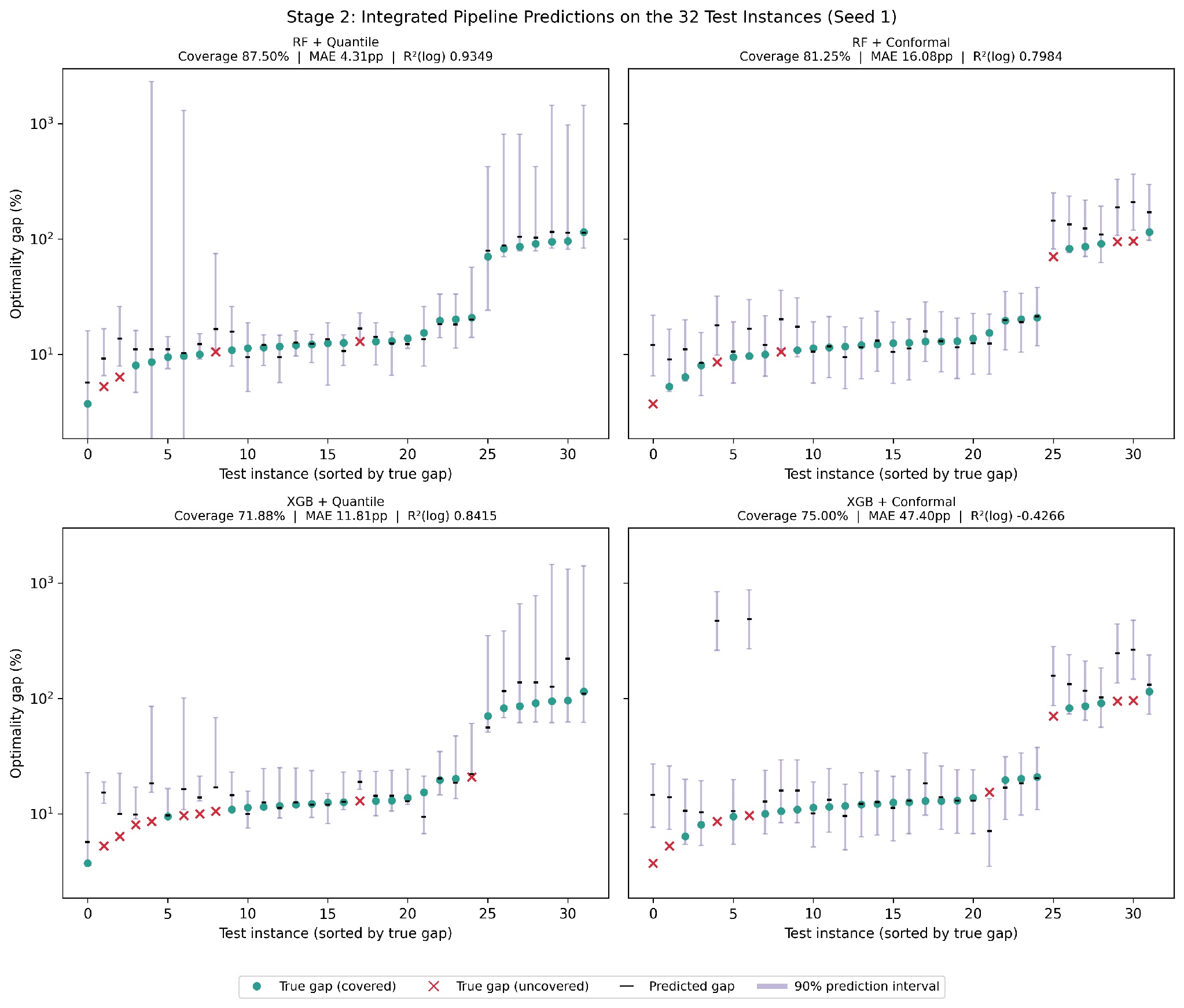
Random Forest + Quantile (abbreviated RF + Quantile in Tables 5 and 7, with XGB for XGBoost likewise) is the strongest of the four: it averages an MAE of 29.5226.01pp and a log-space R2 of 0.8000.082, achieving the lowest MAE of any pipeline on 26 of the 30 seeds. However, its mean coverage of 82.17%6.15% falls somewhat short of the nominal 90%, and its median interval of 14.263.79pp is the second-narrowest. Narrowing to its specific behavior on Seed 1 as shown on Figure 2, it achieves an MAE of 5.21pp, an R2 of 0.9204, and a coverage of 90.63% (29/32), which does meet the nominal target. The three instances that it fails to cover are bays29, ts225, and family_B_clustered_n125_s0, where the model over-predicts the gaps and the actual values lie beneath the lower bound.

Random Forest + Conformal shares the identical RF Stage 1; the distinction lies in Stage 2, where 26 of the 128 training instances are withheld as a calibration set, 102 are used to fit the regressor, and a single conformal score is applied uniformly to every test prediction. That uniformity ended up becoming a drawback, as the interval cannot adapt to instance difficulty. This leads to its median width of 18.834.26pp being wider than its quantile counterpart’s and its MAE of 36.2223.25pp being worse, reflecting in part the accuracy cost of fitting on 102 rather than 128 instances. Still, in return it achieves a mean coverage of 86.34%5.59%, which is closer to nominal than the quantile variant.

XGBoost + Quantile averages an MAE of 33.6824.97pp and a log-space R2 of 0.7680.082. Its mean coverage of 68.88%9.30% is by far the furthest of the four from the nominal 90%, and it reaches nominal coverage on a single seed alone, the worst count of the four models. XGBoost + Conformal instead attains the highest mean coverage of the four at 89.65%6.63%, essentially at nominal, but it has the widest intervals (21.547.52pp) and the worst mean MAE (39.1624.58pp). Its mean R2 value is 0.6640.240, although the R2 actually turns negative on two of the thirty partitions (−0.0522 on Seed 1, for example), which implies that the model sometimes performs worse than a baseline that always predicts the mean log-gap.

The conformal models achieve better coverage over the thirty seeds (Table 5), which is expected given conformal prediction’s design to deliver coverage at the cost of wider intervals. This is not always the case, such as with the Random Forest pair on Seed 1 (90.63% quantile against 75.00% conformal), but the mean across 30 seeds exhibits the trend.

Feature	RF + Quant.	RF + Conf.	XGB + Quant.	XGB + Conf.
mst_weight	0.416	0.350	0.076	0.029
avg_violation_magnitude	0.297	0.335	0.130	0.172
cv_edge_weight	0.097	0.111	0.064	0.591
heuristic_Insertion	0.078	0.082	0.072	0.067
heuristic_CH	0.029	0.024	0.058	0.030
triangle_violation_rate	0.027	0.046	0.087	0.020
heuristic_NN	0.019	0.017	0.082	0.018
edge_weight_skewness	0.011	0.009	0.057	0.008
min_edge_weight	0.008	0.008	0.051	0.008
n​	0.008	0.008	0.039	0.010
pct_short_edges	0.007	0.006	0.053	0.006
heuristic_Greedy	0.004	0.004	0.051	0.013
type_Geo	0.000	0.000	0.059	0.004
type_EUC_2D	0.000	0.000	0.057	0.004
type_Explicit	0.000	0.000	0.065	0.020

On feature importance (Table 6), the Random Forest gap regressor is dominated almost exclusively by mst_weight and avg_violation_magnitude, together 71.3% of its decisions for Quantile Regression and 68.5% for Conformal Prediction. Since both are weakly correlated (r=−0.35), they differ from the domination by triangle-inequality features in Stage 1. Interestingly, the heuristic indicators also contribute about 13% in both models, justifying our choice of predicted heuristic as a Stage 2 feature. However, the XGBoost regressors differ starkly in their feature weights: the quantile variant spreads weight more evenly, led by avg_violation_magnitude (0.130), triangle_violation_rate (0.087), and heuristic_NN (0.082), with type_Explicit only sixth at 0.065; the conformal variant on the other hand concentrates on cv_edge_weight (0.591) and avg_violation_magnitude (0.172).

Statistical Significance

Regardless of demonstrated performance differences between certain models, inferences should be made cautiously. Indeed, differences between per-seed results are paired and subject to direct testing since each seed uses the same partition in all four pipelines. Following the recommendations of Demšar²⁵, whose framework compares different models on multiple data sets rather than on multiple partitions of one data set, we use non-parametric paired tests with a Holm-type correction in case of comparing several learning algorithms with one reference algorithm. Nevertheless, the thirty splits resample the same 160 instances and their test sets overlap, so they are not independent of each other. Therefore, an ordinary paired test would lead to an inflated Type I error rate²⁶. In order to prevent this, we report the corrected resampled t-test of Nadeau and Bengio²⁷ in the form given by Bouckaert and Frank²⁸, as well as the Wilcoxon signed-rank test²⁹ and the ordinary paired t-test. Holm–Bonferroni correction³⁰ is done in every metric category. Random Forest + Quantile is pre-specified as the reference model (Table 7).

Reference: RF + Quantile	Mean diff.	95% CI	dz	Wins	Holm p
MAE (pp), lower is better
vs. RF + Conformal	6.697	[4.453, 8.940]	1.11	29/30	0.1137
vs. XGB + Quantile	4.152	[2.813, 5.491]	1.16	28/30	0.1137
vs. XGB + Conformal	9.633	[5.659, 13.606]	0.91	28/30	0.1137
R2(log), higher is better
vs. RF + Conformal	0.051	[0.026, 0.076]	0.76	21/30	0.4355
vs. XGB + Quantile	0.032	[0.017, 0.047]	0.80	24/30	0.4355
vs. XGB + Conformal	0.136	[0.039, 0.234]	0.52	23/30	0.4355
Median interval width (pp), lower is better
vs. RF + Conformal	4.568	[3.064, 6.073]	1.13	26/30	0.1252
vs. XGB + Quantile	−0.361	[−1.731, 1.009]	−0.10	15/30	0.8546
vs. XGB + Conformal	7.285	[4.302, 10.269]	0.91	26/30	0.1948

As shown in Table 7, it should be noted that none of the tests achieve the significance threshold under Holm correction. The tests closest to significance are those related to MAE comparison, which coincide at p=0.1137 under the monotonicity enforcement of Holm. Likewise, the Stage 1 comparison of the two selectors’ accuracy on the paired data is null (1.67 accuracy points, 14 of 30 seeds, p=0.359). In other words, no statistical claims can be made regarding any of the pipelines being better; Random Forest + Quantile is still recommended solely due to its empirical superiority. For comparison, without taking into account dependence, all 21 of 21 comparisons would have achieved significance, with some reaching unbelievable p<10−6. On the other hand, upon taking the dependence into account, the MAE advantage of Random Forest + Quantile over XGBoost + Quantile changed from p=6.310−7 to p=0.038.

However, it should be mentioned that this is an example of underpowered tests, rather than strict proof that the methods are equivalent. The minimum detectable standardized effect size is |dz|=1.09 and even |dz|=1.35 under Holm correction, while all 12 main pairwise tests have smaller absolute effect sizes than 1.35. This cannot be remedied by increasing the number of seeds since the inflation factor is bounded below by the ratio of test-to-training sample sizes: as k, the minimum effect size only decreases to |dz|=0.98. Overall, the main issue is the limited size of the library, which has only 160 instances; one of the conclusions from this analysis is that the extension of the dataset would be beneficial.

Finally, one inferential conclusion regarding internal validity does survive. When applying the one-sample Wilcoxon signed-rank test²⁹ to compare each pipeline’s per-seed coverage against the target value of 90%, it can be seen that XGBoost + Quantile is significantly miscalibrated, failing to achieve nominal coverage by 21.12 percentage points and obtaining the nominal coverage on only 1 of 30 seeds (Holm p=0.0008). On the other hand, neither of the conformal pipelines is statistically significantly miscalibrated, while Random Forest + Quantile under-covers by 7.83 percentage points, which is also not significant (p=0.0705). It is obvious that conformal calibration provides the coverage property of the methodological design, while Quantile intervals are narrower and lack such a property. The trade-off from both perspectives is demonstrated by Fig. S1 in the Supplementary Material.

Computational Cost of Feature Extraction

First of all, our framework relies on the crucial assumption about structural features being cheaper compared to the heuristics that they replace. An obvious concern is that some structural features have the same asymptotic complexity as the heuristics—minimum spanning tree takes O(n2), whereas pct_short_edges is O(n2logn); however, it should be stressed that the bottleneck of heuristics is dominated by Christofides and Insertion, which have complexity of O(n3). As a result, as n grows, feature extraction will become more time-efficient than executing all heuristics. To identify the conditions when our assumption holds, we measured the execution time of the feature vector and heuristics on the training instances. Timing was done for the whole feature vector and each heuristic on a single machine using a monotonic wall-clock timer.

   

The timing was done on 130 benchmarked instances with n800 for which all four heuristics ran to completion. On average, the framework is 15.86 faster than executing all four heuristics, and this advantage grows monotonically as n grows—from 0.52 for n130 to 62.73 for 501n800 (supplementary Table S9). There are two interesting observations. Firstly, the framework is slower below roughly n=150 because feature extraction involves a constant cost independent of n, while all heuristics complete execution in milliseconds at small n. Secondly, the constant cost is dominated by the two Monte Carlo triangle-inequality features, which take 98.2% of the total extraction time because each samples 200,000 triples independent of instance size. Since the 200,000 triples were chosen manually, changing the sample size could reduce the threshold well below n=150.

It can be seen that with growing instance size the tradeoff emerges. In an extreme example, consider the 15 instances for which execution timed out, summing up to 23 rows; these instances are impractical because Insertion (15) and Christofides (8) run for more than 600,000 ms. Obviously, executing feature extraction is more efficient than executing all heuristics in this case, which supports our model at bigger instance sizes. These results are presented in supplementary Table S10. Overall, our framework is still justified given its applicability for large instances, although it is limited for smaller ones.

Validation and Robustness

Scale invariance. Rescaling 154 of the 160 dataset instances (the remaining six could not be re-sourced from their original files) by factors of 0.01, 10, and 1000 and passing them through both trained stages leaves the predicted heuristic unchanged in 458 of 462 tests and reproduces the predicted gap exactly in 396 of 462. Every mismatch occurs at the extreme 0.01 factor out of the three. At 0.01 specifically, 67 of the 154 instances (43.5%) show some mismatch, with gap differences of 2.9% relative on median (up to 16.4%); however, the heuristic decision itself changes in only 4 of 154 cases. All mismatches are due to a floating-point comparison in the triangle-inequality check which carries no tolerance. Indeed, on near-metric instances, sampled triples within rounding error of equality can flip across the strict inequality once every distance is shrunk by two orders of magnitude (Supplementary Table S11). This is a numerical precision issue, rather than features holding any scale dependence.

Generalization across instance families.  As we restrict evaluation to the 105 original TSPLIB instances alone, cross-validation reaches 76.19% against the 70.48% always-Christofides baseline for that subset. This is a moderate increase, which shows that the model does not strictly depend on the generated instances but is strongly influenced.

Still, the framework does not survive withholding an entire synthetic family. Withholding the random family (which is 100% Greedy) gives 0% accuracy against a 100% majority baseline; the clustered family gives 76.92% accuracy when withheld and tested, while christofides_hard gives 86.21%, each exactly matching its own majority baseline, so the model shows no advantage either; and TSPLIB gives 17.14% against 70.48% (supplementary Table S12), which is worse than trivial. We located the cause with a model-agnostic control (Table S13 of the supplementary material). Taking each held-out instance’s nearest training instance in standardized feature space, the label matches only 7.7–16.2% of the time, and that neighbor sits 6 to 9 times farther away than a typical within-dataset neighbor gap. We can conclude that the problem is in training coverage, and not because our model was leaning on any fragile patterns. We bound our claim accordingly: structural features predict heuristic performance for instances drawn from the mixture of regimes this benchmark represents, and not zero-shot transfer into an unfamiliar geometric regime.

Stage 1 to Stage 2 error propagation. Since in Protocol B Stage 2 uses Stage 1’s predicted heuristic as an input feature, it is worth measuring the error propagation between the models. We ran each pipeline twice on the identical split: as deployed receiving the predicted heuristic from Stage 1, and as an oracle receiving the true best heuristic. Three of the four pipelines achieved a lower MAE in our deployed model than under the oracle, by 0.65 to 1.42pp. Only XGBoost + Quantile deployed worse than its oracle by 5.88pp; it also has the weakest Stage 1 accuracy on this partition, so it exposes more and more varied misclassifications. Supplementary Table S14 gives both configurations for all four pipelines.

This result seems counterintuitive, as receiving the true best heuristic should produce better results than a direct passing from Stage 1. This actually turned out to be because the Stage 2 model scores the optimality gap against the classified heuristic, and as the heuristic given to Stage 2 for a certain instance changes, the accuracy of the model is affected. Random Forest’s Seed-1 errors are four true-Greedy instances predicted as Christofides, so the oracle must predict Greedy gaps on them, which is scarcer and harder-to-model (31 training instances) than Christofides (75 training instances), while the deployed pipeline predicts the better-modeled Christofides gaps. XGBoost + Quantile’s six misclassifications include two beyond this pattern, for which the wrong classification does not benefit the prediction gap. End-to-end gap estimates are therefore not systematically degraded by imperfect selection, but rather reflects which instances get misclassified and how well their substituted heuristics are modeled. This result again corroborates our previous conclusion on how an extended dataset can improve the model.

Discussion

Considering all pipelines, we move on to finding appropriate ones to use. It is already evident that no pipeline shows statistical advantage over others; hence, this part of the work is aimed at practicality and performance evaluation, referring to Stage 1 comparison from Table 3 and Stage 2 comparison from Table 5 provided above.

Heuristic Selection

All three learned selectors show the mean cross-validation accuracy from 79.38% to 80.00%, comfortably outperforming the type-based rule and single-best-solver baseline. It indicates that cheap instance features can be used to predict optimal heuristics. At that, difference between any two selectors does not exceed 0.62 percentage points, which is well within fold-to-fold variability; therefore, one cannot claim the superiority of accuracy of any of selectors, but rather separate them on the basis of regret. However, the regret of the unconditional application of the most frequent optimal heuristic Christofides amounts to 1.849 versus the 0.028 of Random Forest, a 66-fold decrease, and catastrophic failures go down to 0.63% from 23.68%. Indeed, in the comparison of the fixed rule and our models accuracy proves to be an insufficient criterion because the rule tends to yield much too expensive errors and should be considered from the perspective of regret. Logistic regression does not prove to be competitive, yielding more than fourfold regret compared with each of two tree ensembles; otherwise, both tree ensembles have similar regret, though XGBoost shows stronger fold-to-fold deviation, more dependence on hyperparameters, and the largest train–CV gap among the three. Consequently, Random Forest appears to be more resistant according to these results.

Gap Prediction Quality

As for point accuracy, the Random Forest combined with Quantile Regression appears to be the strongest Stage 2 model (Table 5): it gives the lowest mean MAE and the highest log-space R2 among the thirty seeds despite non-optimal calibration. Indeed, both conformal variants come closer to the nominal 90% coverage. The leadership of Random Forest + Quantile stays consistent upon repeated runs, yielding the lowest MAE 26 out of 30 seeds. Still, the magnitude comparison between the Seed-1 values does not confirm such dominance as a general one since Seed 1 corresponds to a good run within a more general distribution.

Final Pipeline

We choose Random Forest + Quantile Regression for the point accuracy as the model having the lowest mean MAE and the highest log-space R2, performing competitively in other criteria and having the smaller train–CV gap compared with XGBoost. Still, when the prediction interval becomes necessary rather than the point estimate, the conformal approach should be used since both approaches give statistically indistinguishable coverage from the nominal while Random Forest + Quantile does not. Ultimately, we refrain from crowning any model as singularly statistically best, as discussed in the Statistical Significance section above.

Practical Deployment Guidance

We will provide guidance for deployment based on the results obtained above. The decisive attribute for deploying the framework is the instance size: below around n=150 the framework is counter-productive due to the fixed cost of feature extraction; the opposite happens beyond this threshold and is growing with size. On which pipeline to use, we advise Random Forest + Quantile for a point estimate, assuming that this one has margin of the same sign, but noting that it does not have complete statistical evidence; correspondingly, where the interval is required, we would suggest a conformal alternative, since they both achieve closer coverage to nominal compared to the Quantile models. On which output is reliable, we consider the Random Forest Stage 1 model to produce the more trustworthy output, as its errors are close ties with XGBoost’s, while for Stage 2 the interval should be considered, not the point value. For Stage 2, we advise not taking into account single-partition MAE numbers as expected performance on new instances, as the log-space R2 metric is a more stable summary. Finally, it is necessary to consider Monte Carlo sample size first in case of adopting the framework, which was not optimized but chosen conservatively and now dominates the cost of feature extraction for small instance sizes.

Overall, this research has explored the possibility of using cheaply computable structural features of the TSP instance to predict both the best-performing construction heuristic and the expected optimality gap without applying any heuristic beforehand. The results indicate they can perform this task within certain limitations of three kinds: the scope of applicability of the framework, the strength of the evidence behind the reported figures and quality of the features themselves.

Scope of applicability

Firstly, “the best” implies the best of the 4 construction heuristics considered here; other tour-construction and tour-improvement methods do not belong to the pool. Secondly, all 160 instances lack diagonal entries and retain the symmetrical structure, thus the asymmetric TSP remains untested. Consequently, several features, including the minimum spanning tree weight, are defined for undirected graphs, and would need to be redefined for expansion of scope. Finally, the problem is assumed to be in the form of a complete weighted graph with known static distance matrix, while the real-life routing problems with time windows, vehicle capacities or road networks violate this assumption. Ultimately, the contribution is limited to the application to classical TSP instances in the form of explicit or coordinate-derived distance matrices, symmetric and with or without metric structure.

Strength of evidence

The current dataset consists of only 160 instances, of which 55 Explicit instances are artificially generated in order to provide variation in the dataset besides the TSPLIB; this is a beneficial characteristic in terms of extending our scope to non-metric instances and thus investigating more complex feature influences, such as triangle violation rate, but from the practical standpoint these instances do not represent real-world TSP instances distribution. The numbers reported should thus be considered the evidence of viability on this particular benchmark (instances similar to our training set, such as Euclidean coordinate-derived instances, Geo instances, and artificial Explicit instances, generated via comparable algorithm) and not generalizable performance guarantee on new, differently structured instances. This is also supported by the analysis of leave-one-family-out, where the classifiers, though not relying on provenance labels for different families represented in the training data, failed to extrapolate to the instance family left out of the training completely. Apart from this, we mention a possible limitation of the measured optimality gap for a number of instances in our training dataset: Concorde has proved the optimality for most of instances, but the remaining ones use LKH tours as the reference, and their optimality gaps should be seen as approximate estimates rather than exact measure. Moreover, even averaged across 30 partitions the gap figures prove to be very broad ranging, with integrated MAE between 2.83 and 73.74pp (Table 5), since there are only a few adversarial instances with gaps three orders of magnitude higher than the median – resulting in logarithmic-space R2 (0.8000.082) being the preferable summary metric. These partitions also prove pipeline comparisons directionally consistent but not statistically significant; we discussed the potential for improvement of this issue through expansion of instance library. Lastly, we mention Nearest Neighbor to have only 8 optimal instances and be unrecoverable for all selectors (resulting in per-class F1 equal to zero), showing the limitation of class imbalance problem; however, this is also expected since this method performs poorly on most instances. We conclude that revision of the set of heuristics for selection to be more balanced is one of the issues that can be improved in future works.

Feature set

Here, the Stage 2 predictions coincide perfectly in 396 out of 462 attempts at rescaling, with some discrepancies among the others but with only 4 of them changing the recommended heuristic itself. As was mentioned earlier, the reason for this is the rounding in the triangle inequality sampling procedure, and it is awaiting a tolerance-based fix. Nevertheless, independently of it, when considering certain features, we have to point out that pct_short_edges is of limited usefulness, containing little of the information about the edge lengths that we would expect from it, with the value fixed around 0.10 (mean 0.102, standard deviation 0.011) due to the construction. In turn, the nonzero permutation importance of this feature, 0.043, is more a weak indicator of tie heavy Explicit instances. Further, three pairs of features are strongly correlated (Feature Diagnostics and Collinearity, above), with variance inflation factors reaching 84.12. This means that due to certain deficiencies in the feature set, the effective dimensionality is closer to five rather than to nominal nine. However, it does not affect predictive performance, as the tree ensembles handle correlated variables, but only restricts the feature importance of the feature in question. Still, pruning the redundancy would give a more parsimonious model.

In general, broadly speaking, the two-stage pipeline proposed above is a generalizable architecture for the solution of other algorithm selection problems, one of the further areas for extension. Ultimately, the results support our claim, albeit with scope limitations, about using cheap structural features, chosen without running any heuristic beforehand, to select heuristics on the instances like these studied here. Expanding this hypothesis to the further instance families, larger dataset and other combinatorial problems is the natural further step for this research.

Supplimentary Material

References

1. W. R. Hamilton. Account of the icosian calculus. Proceedings of the Royal Irish Academy. Vol. 6, pg. 415–416, 1856. [↩]
2. R. M. Karp. Reducibility among combinatorial problems. 50 years of integer programming 1958–2008. Springer Berlin Heidelberg, 2010, https://doi.org/10.1007/978-3-540-68279-0_8. [↩]
3. P. Kerschke, H. H. Hoos, F. Neumann, H. Trautmann. Automated algorithm selection: survey and perspectives. Evolutionary Computation. Vol. 27, pg. 3–45, 2019, https://doi.org/10.1162/evco_a_00242. [↩]
4. D. H. Wolpert, W. G. Macready. No free lunch theorems for optimization. IEEE Transactions on Evolutionary Computation. Vol. 1, pg. 67–82, 1997, https://doi.org/10.1109/4235.585893. [↩]
5. J. R. Rice. The algorithm selection problem. Advances in computers. Vol. 15, Elsevier, 1976, https://doi.org/10.1016/S0065-2458(08)60520-3. [↩]
6. L. Xu, F. Hutter, H. H. Hoos, K. Leyton-Brown. SATzilla: portfolio-based algorithm selection for SAT. Journal of Artificial Intelligence Research. Vol. 32, pg. 565–606, 2008, https://doi.org/10.1613/jair.2490. [↩]
7. K. Smith-Miles, M. A. Muñoz. Instance space analysis for algorithm testing: methodology and software tools. ACM Computing Surveys. Vol. 55, pg. 1–31, 2023, https://doi.org/10.1145/3572895. [↩]
8. L. Kotthoff. Algorithm selection for combinatorial search problems: a survey. Data mining and constraint programming: foundations of a cross-disciplinary approach. Springer International Publishing, 2016, https://doi.org/10.1007/978-3-319-50137-6_7. [↩]
9. O. Mersmann, B. Bischl, H. Trautmann, M. Wagner, J. Bossek, F. Neumann. A novel feature-based approach to characterize algorithm performance for the traveling salesperson problem. Annals of Mathematics and Artificial Intelligence. Vol. 69, pg. 151–182, 2013, https://doi.org/10.1007/s10472-013-9341-2. [↩]
10. F. Hutter, L. Xu, H. H. Hoos, K. Leyton-Brown. Algorithm runtime prediction: methods & evaluation. Artificial Intelligence. Vol. 206, pg. 79–111, 2014, https://doi.org/10.1016/j.artint.2013.10.003. [↩]
11. H. H. Hoos, T. Stützle. On the empirical scaling of run-time for finding optimal solutions to the travelling salesman problem. European Journal of Operational Research. Vol. 238, pg. 87–94, 2014, https://doi.org/10.1016/j.ejor.2014.03.042. [↩]
12. D. J. Rosenkrantz, R. E. Stearns, P. M. Lewis II. An analysis of several heuristics for the traveling salesman problem. SIAM Journal on Computing. Vol. 6, pg. 563–581, 1977, https://doi.org/10.1137/0206041. [↩]
13. D. S. Johnson, L. A. McGeoch. The traveling salesman problem: a case study in local optimization. Local search in combinatorial optimization. John Wiley & Sons, pg. 215–310, 1997. [↩]
14. N. Christofides. Worst-case analysis of a new heuristic for the travelling salesman problem. Operations Research Forum. Vol. 3, pg. 20, 2022, https://doi.org/10.1007/s43069-021-00101-z. [↩]
15. A. R. Karlin, N. Klein, S. Oveis Gharan. A (slightly) improved approximation algorithm for metric TSP. Proceedings of the 53rd Annual ACM SIGACT Symposium on Theory of Computing. pg. 32–45, 2021, https://doi.org/10.1145/3406325.3451009. [↩]
16. G. Reinelt. TSPLIB—a traveling salesman problem library. ORSA Journal on Computing. Vol. 3, pg. 376–384, 1991, https://doi.org/10.1287/ijoc.3.4.376. [↩]
17. L. Breiman. Random forests. Machine Learning. Vol. 45, pg. 5–32, 2001, https://doi.org/10.1023/A:1010933404324. [↩]
18. T. Chen, C. Guestrin. XGBoost: a scalable tree boosting system. Proceedings of the 22nd ACM SIGKDD International Conference on Knowledge Discovery and Data Mining. pg. 785–794, 2016, https://doi.org/10.1145/2939672.2939785. [↩]
19. D. L. Applegate, R. E. Bixby, V. Chvátal, W. J. Cook. The Traveling Salesman Problem: A Computational Study. Princeton University Press, 2006. [↩]
20. K. Helsgaun. An effective implementation of the Lin–Kernighan traveling salesman heuristic. European Journal of Operational Research. Vol. 126, pg. 106–130, 2000, https://doi.org/10.1016/S0377-2217(99)00284-2. [↩]
21. N. Meinshausen. Quantile regression forests. Journal of Machine Learning Research. Vol. 7, pg. 983–999, 2006. [↩]
22. V. Vovk, A. Gammerman, G. Shafer. Algorithmic Learning in a Random World. Springer, 2005, https://doi.org/10.1007/b106715. [↩]
23. J. Lei, M. G’Sell, A. Rinaldo, R. J. Tibshirani, L. Wasserman. Distribution-free predictive inference for regression. Journal of the American Statistical Association. Vol. 113, pg. 1094–1111, 2018, https://doi.org/10.1080/01621459.2017.1307116. [↩]
24. C. Strobl, A.-L. Boulesteix, T. Kneib, T. Augustin, A. Zeileis. Conditional variable importance for random forests. BMC Bioinformatics. Vol. 9, art. 307, 2008, https://doi.org/10.1186/1471-2105-9-307. [↩]
25. J. Demšar. Statistical comparisons of classifiers over multiple data sets. Journal of Machine Learning Research. Vol. 7, pg. 1–30, 2006. [↩]
26. T. G. Dietterich. Approximate statistical tests for comparing supervised classification learning algorithms. Neural Computation. Vol. 10, pg. 1895–1923, 1998, https://doi.org/10.1162/089976698300017197. [↩]
27. C. Nadeau, Y. Bengio. Inference for the generalization error. Machine Learning. Vol. 52, pg. 239–281, 2003, https://doi.org/10.1023/A:1024068626366. [↩]
28. R. R. Bouckaert, E. Frank. Evaluating the replicability of significance tests for comparing learning algorithms. Advances in Knowledge Discovery and Data Mining (PAKDD 2004), Lecture Notes in Computer Science. Vol. 3056, pg. 3–12, Springer, 2004, https://doi.org/10.1007/978-3-540-24775-3_3. [↩]
29. F. Wilcoxon. Individual comparisons by ranking methods. Biometrics Bulletin. Vol. 1, pg. 80–83, 1945, https://doi.org/10.2307/3001968. [↩] [↩]
30. S. Holm. A simple sequentially rejective multiple test procedure. Scandinavian Journal of Statistics. Vol. 6, pg. 65–70, 1979. [↩]