A Study of the Impact of Land Use Land Cover Change on Maheshkhali Upazila’s Forest Area Using Normalised Difference Vegetation Index Trends and Supervised Classification

Abstract

Coastal forests are a very important part of the coastal ecosystems. Maheshkhali Upazila is the only offshore hilly island in Bangladesh that has a sizable mangrove forest along its coasts as well as hilly upland forests. Unfortunately, coastal forests have been in decline globally for the last few decades. To assess how the forest area of Maheshkhali Upazila has been affected, the Normalised Difference Vegetation Index (NDVI) and Supervised Classification based on the Random Forest method were applied to the island. The years from 2004 to 2024, during the dry season (November-February), were used for NDVI analysis. Sensor-specific NDVI trends differed between satellite generations, but the statistical fits were weak and the trends for Landsat 8 and 9 were not statistically distinguishable from zero. NDVI trends alone can mask land-cover change or deforestation, so supervised classification was also performed. Classification of 2020, 2022, and 2024 shows the forest area decreasing while Aquaculture (5), Agriculture (3), and Built-up (2) areas increase. Classification accuracy was assessed against an independent reference dataset of 1,000 points interpreted on high-resolution imagery, and areas were corrected for classification error following Olofsson et al. (2014). This yielded a probable forest decline of approximately 11 km² (95% CI: −3.6 to +24.9 km²), considerably smaller than the unadjusted estimate and not statistically significant. Ground-truth field data were unavailable, which remains an important limitation. 

Introduction

Coastal forests such as mangroves provide ecosystem services whose loss to coastal land conversion carries substantial economic cost^1,2,3. The  Bengal delta encompasses a large part of the coastal area and is the second largest delta in the world⁴. Due to its extensive coastal area, mangrove-dominated ecosystems and coastal forests in Bangladesh are of great importance to the region. They provide essential ecosystem services like carbon sequestration and shoreline stabilisation, supporting local livelihoods^5,6. 

Mangrove protection and restoration are responsive to ecosystem management in and around the tidal zone⁷. The conservation and restoration of mangrove ecosystems is critically important for protecting marine life and vegetation. This study uses land use/land cover (LULC) change as a direct indicator of anthropogenic pressure on coastal ecosystems, such as mangrove forests and hilly upland forests, and aims to document forest degradation in Maheshkhali Upazila, where data and research are lacking.

Maheshkhali is the only offshore hilly island in Bangladesh, situated on the southeastern coast. The island, along with a few adjacent islands, has its own administrative Upazila⁸. The Upazila features a unique geological system towards the eastern cliffy coast of Bangladesh that is characterised by hilly terrain encircled by coastal plain landforms ⁹. The island exhibits coastal plains and active depositional systems, which together determine both its ecological role and its vulnerability to shoreline change¹⁰. 

Recent research on LULC change of Maheshkhali Upazila is limited^11,12. For this area, a study comparing NDVI trends from multiple Landsat imagery, combined with LULC change data collected using supervised classification, has not been conducted before. This study aims to (1) assess the loss of forest area in Maheshkhali Upazila and identify its primary drivers, using remote sensing approaches including NDVI trend analysis and supervised classification, and (2) evaluate the usefulness of these remote sensing methods for detecting and quantifying forest area loss.

This study uses the administrative boundary of Maheshkhali Upazila as the AOI, which actually includes a few islands instead of one. Using Landsat 5, 7, 8 and 9 imagery, the NDVI trends of each year in the dry season, i.e., the months of November to February between 2004 and 2024, have been analysed using R and Google Earth Engine.

Maheshkhali’s coastal habitats and the increasing development pressures in the region hold great importance for nature and people. For this reason, a focused, reproducible assessment using a consistent multi-sensor Landsat time series can inform conservation, aquaculture zoning, and coastal management⁸. In this study, through the use of open-source data and tools like Google Earth Engine and Landsat imagery, the causes of deforestation and human land-cover change will be discussed and interpreted. With the outcomes of this research, it is aimed to fill a long-lasting gap in LULC change data of Maheshkhali Upazila.

Literature Review

This section summarises prior research on the specific methods used in this paper, i.e., NDVI analysis, random forest method, and supervised classification, relevant studies of the region, mangrove landscape change worldwide, and studies on the LULC change of the research area in previous years.

In the field of remote sensing, different vegetation indices have been in use for a long time to monitor forest and agricultural health and change. Normalised Difference Vegetation Index (NDVI) is one such index, which is derived from near-infrared and red reflectance: 

In Landsat

In Landsat 8-9,

¹³.

NDVI is one of the most globally favoured vegetation indices used widely for research purposes, i.e., vegetation monitoring, crop studies, and deforestation^14,15,16.

As much as NDVI is favoured by researchers, it has several limitations. First, its behaviour is landscape-dependent: a recent hyperspectral study shows that although various vegetation indices remain highly correlated with NDVI, their perceptual and structural responses can differ significantly, and NDVI’s discriminative power is low in heterogeneous areas¹⁶. This means NDVI can obscure vegetation transitions on an island like Maheshkhali, where Agriculture (3), Aquaculture (5), and Forest (0) overlap and interchange regularly. Second, NDVI is sensitive to climate rather than land cover alone; vegetation greenness responds to rainfall¹⁷, an effect that is pronounced in the tropical monsoon setting of Maheshkhali and is supported by South Asian studies where over 70% of areas show a positive NDVI–rainfall correlation¹¹. Third, NDVI values differ between sensors owing to differences in spectral band characteristics, radiometric calibration, and detector design, as documented for Landsat-7 ETM+ and Landsat-8 OLI¹⁸; when multi-decadal imagery from multiple sensors is combined, these differences can introduce artificial trends¹⁹. NDVI is additionally affected by soil background, temperature, atmospheric noise, and substratum reflectivity, and it saturates when the Leaf Area Index exceeds 3, limiting its ability to distinguish variation in dense vegetation²⁰. Together, these limitations mean that on a dynamic, heterogeneous island like Maheshkhali, changes in NDVI may not directly correspond to changes in forest area. 

Due to these limitations of NDVI, it is not a wise decision to analyse land-cover change based on NDVI trends only. Supervised Classification is another method to classify land-cover change, which has been very popular in recent years. Supervised Classification is a machine learning method where an algorithm learns to categorise data by training on labelled examples. There are various algorithms in use for supervised classification, i.e., Random Forest, Support Vector Machine, and Classification and Regression Trees. Among them, Random Forest produces the most accurate results according to a recent study^21,22. According to another study, Random Forest also outperforms a single Decision Tree and is less sensitive than other streamlined ML Classifiers to the quality of training samples and to overfitting, due to the large number of Decision Trees produced by randomly selecting a subset of training samples and a subset of variables for splitting at each tree node²². Moreover, Random Forest can also successfully handle high data dimensionality and multicollinearity, although it’s sensitive to sampling design^23,24. 

Google Earth Engine (GEE) is a cloud-based geospatial analysis platform developed by Google. GEE is a popular platform to monitor deforestation and land use change. In GEE, temporal aggregation of time-series imagery yields higher accuracy than analyses based on single-date images^25,26. According to another study, GEE is a reliable and powerful tool for ML classification^27,28,22.

Mangrove forests have been in decline worldwide over the past few decades. According to a recent study, globally, mangrove forests have declined by 30-50% over the past half-century². Since 1980, 3.6 million ha of mangrove forests have been lost. Among these, 1.89 million ha have been lost to coastal aquaculture, and 1.4 million ha were lost due to shrimp culture⁷. The majority of mangrove deforestation happened in the continent of Asia, where shrimp farming accounts for 1.2 million ha of mangrove forest loss ²⁹. Even in Bangladesh, mangrove forests have been decreasing over the past few decades^30,31,32. From 2005-2015, 36 km² of coastal area of the eastern coast of Bangladesh have been lost due to erosion, among which a portion is a coastal mangrove forest^10,30. In Maheshkhali Upazila, shorelines have changed due to global temperature and sea level rise, sediment transportation, environmental intervention, cyclones, and coastal flooding, among other reasons³³. Moreover, a previous study also expected that megaprojects like Matarbari would affect mangroves, wetlands, and sandy beaches due to their proximity to ecologically sensitive zones such as Sonadia Island³⁴. Coastal areas are also depicted as the most suitable for coastal aquaculture^5,35,36, such as salt pans and shrimp farms. As a result, Maheshkhali Upazila has seen a lot of deforestation in the past few years, the majority of which is mangrove forest^33,37,38.

Methods

In this study, we have used a longitudinal, multi-temporal remote sensing approach, combining NDVI trend analyses with random forest-based supervised machine learning classification, based on imagery from 4 Landsat satellites over a period of over 20 years. Only open-source free data and tools, like Google Earth Engine and R, have been used in this paper.

Case Study of Area: Maheshkhali Upazila

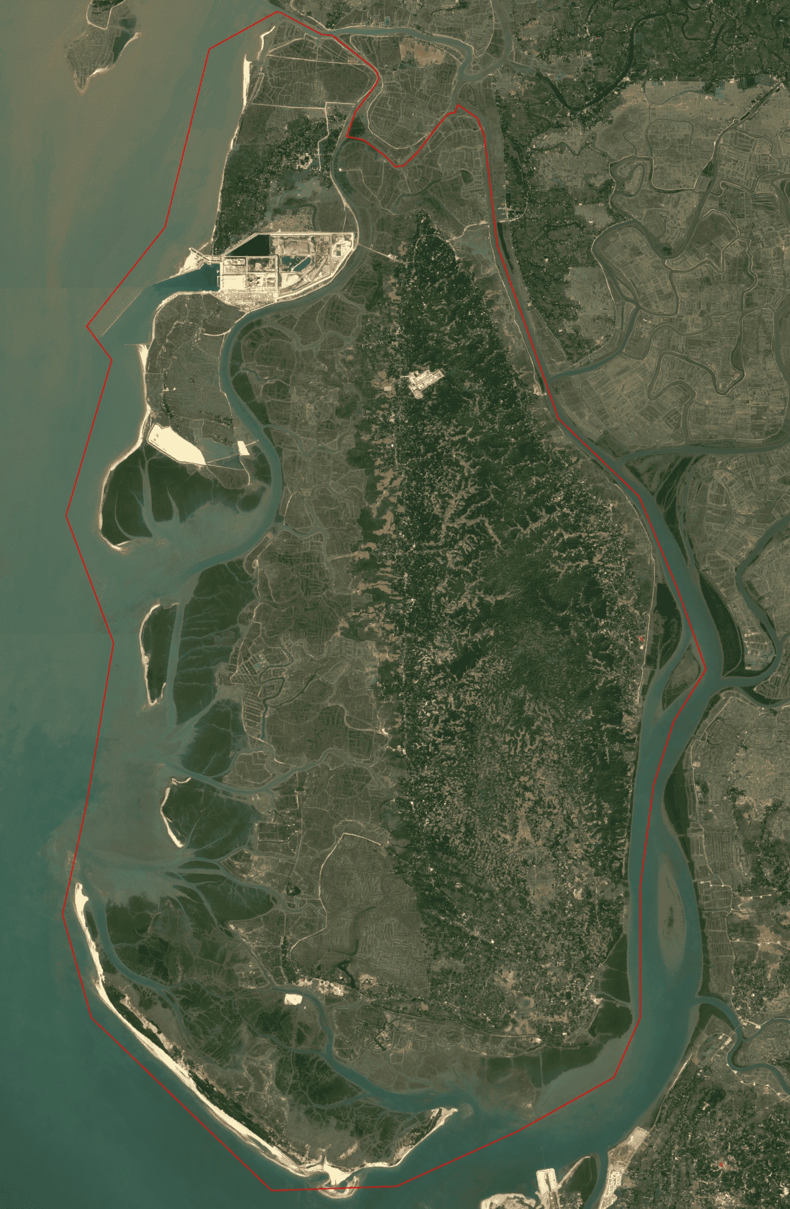
Maheshkhali Upazila (Figure 1), the only hilly island in Bangladesh, which also has a large area of mangrove forest along its coasts, is situated in the district of Cox’s Bazar along the southeastern coast of Bangladesh. The river Bakkhali separates the island from Cox’s Bazar Upazila. Maheshkhali is also its own separate administrative Upazila. The geographic location of the island is 21° 30′ 0″  N to 21° 15′ 0″ N latitude and 91° 50′ 0″ E to 92°5’0” E longitude. The island has a total area of 388.5 km². The island borders the Bay of Bengal in its western and southern parts. The north of the island is bordered by Pekua, the north-east is bordered by Chakaria, and the south-east side of the island is bordered by Cox’s Bazar. The island also has other small islands considered part of it, such as Matarbari and Sonadia  . 

The island has been seeing net accretion (i.e., net gain in land) since 1972 at a rate of 1.2 km² per year. This means that, on average, the amount of land accreted surpasses the amount of land eroded every year. This also indicates that the percentage of water bodies around the island might be decreasing each year.

Maheshkhali is situated in a tropical climate zone, affected by the southern monsoon. The island has a total population of 385,500³⁹. The people of the island, especially the native people, rely on salt cultivation and shrimp farming as their prime occupation. The island has also seen some megaprojects take place, such as a deep-sea port and a coal power plant. These megaprojects also threaten the diverse ecosystem of the island, including the mangrove forests on its coastal side. 

Data, Pre-processing, and Analysis

Definition of the Area of Interest (AOI)

We have used the administrative boundary of Maheshkhali Upazila and some of its adjacent water bodies as the AOI of this study (Figure 1). It was prepared as a vector polygon, which was uploaded into GEE as a private asset. To ensure consistency in datasets across time, we have clipped all spatial analyses to the AOI. To confirm spatial accuracy, the AOI boundary has been visually compared and overlaid on the satellite imagery.

Satellite Data

This study used multi-temporal surface reflectance imagery from Landsat Collection 2 Level-2, which we acquired from the four sensors – Landsat 5 TM, Landsat 7 ETM+, Landsat 8 OLI, and Landsat 9 OLI-2. We analysed the periods from November 2004 to February 2025, with analysis from November to February months only in this time period to align with the dry season, minimizing cloud cover. 

Collection 2 Level-2 products were selected to get atmospherically corrected surface reflectance values. The reflectance bands were also rescaled using official scale factors and offsets [reflectance = SR ✕ 0.0000275 – 0.2], and a common set of spectral bands with Blue, Red, Green, Shortwave Infrared 1, Near Infrared, and Shortwave Infrared 2 were constructed for all sensors to sensor-harmonize the data.

We decided to use Landsat because of its long time series. This aligns with past work¹⁵. 

Cloud and Shadow Masking

QA_PIXEL band, which was provided in the Landsat Collection 2 Level-2 products, was used to remove cloud and cloud-shadow contamination. Pixels flagged as cloud (bit 3) or cloud-shadow (bit 4) were excluded, and the mask was applied across all sensors consistently to minimize atmospheric noise, which helped to ensure temporal comparability.

Seasonal Window Selection

Only the dry season months of November, December, January, and February (November to February) of the Bangladeshi winter season were analysed to reduce the impact of monsoon, i.e., cloud cover, rain, and vegetation variability. Generally, vegetation is consistent during the dry season (i.e, winter) in the region. For coastal and tropical vegetation research, this period is widely considered suitable. Each ‘season year’ in this study was considered from November of year Y to February of year Y+1. However, this may underrepresent seasonally active land use cases, especially summer-dependent agricultural crop cycles and monsoon flooding.

Trend Analysis of NDVI

Per scene NDVI time series (Google Earth Engine)

We used a per-scene approach for the NDVI trend analysis. This approach was used instead of using only annual composites. And we calculated NDVI for each Landsat scene using the standard formula:

Over the AOI, each NDVI image was spatially averaged using a reducer of mean in 30 m resolution, and the per-scene mean NDVI value was obtained. In a FeatureCollection containing acquisition date, satellite identifier, and mean NDVI, we stored these values.

In GEE, scatterplots were created that only used the acquisition dates of the imagery to display the temporal variability in NDVI without interpolating between acquisition dates. To investigate cross-sensor differences and possible discontinuities at the time of sensor transitions, other scatterplots were generated that binned NDVI by satellite sensor. 

Seasonal NDVI Composites and Statistics

Annual seasonal NDVI composites for each season year between 2004 and 2024 were generated, complementing per-scene analysis. For each season year, all valid Landsat scenes from the November to February window were combined across sensors, and then they were aggregated to the median value for each season year. In order to reduce residual clouds, Landsat 7 SLC-off gaps and outliers, median compositing was used.

A summary of statistics was extracted over the AOI, and the NDVI was calculated from each seasonal composite. The summary includes mean, standard deviation, minimum, maximum, the 5th, 25th, 50th, 75th, and 95th percentiles. These statistics were also stored as a FeatureCollection and then exported for further analysis.

NDVI Analysis in R

From GEE, the NDVI per scene values were exported to be further analyzed in R. The dates were standardized into the standard date format, and scatter plots of NDVI against time were made.

NDVI values were separated by Landsat sensors, and individual linear models were fitted for each sensor to investigate sensor-specific behavior. Coefficient of determination (R²), p-values, and trend slopes were computed and then compared.

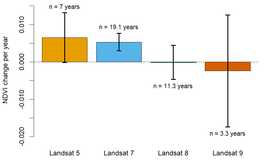
The plots produced are: scatterplot of NDVI trend from the year 2004 to 2024, scatterplot of NDVI trend from the year 2004 to 2024 for each of the 4 satellites’ imagery, and bar chart of NDVI change per year for each of the satellites.

Supervised Land Use Land Cover Classification

Creation of Training Data

Six Land Use and Land Cover (LULC) classes, Forest (0), Water (1), Built-up (2), Agriculture  (3), Bare/Other (4), and Aquaculture(5), were assigned the class codes 0, 1, 2, 3, 4, and 5, respectively. They were digitized manually into polygon features for the six LULC classes. To place the polygons over the spectrally homogeneous areas and ensure class purity,  the true-color imagery, along with index layers (e.g., NDVI, Normalized Difference Water Index (NDWI), Normalized Difference Moisture Index (NDMI), and Normalized Difference Built-up Index (NDBI)), were used. Through preparing separate training datasets for the years 2020, 2022, and 2024, temporal changes in the characteristics of LULC were addressed. Training polygons were digitised manually for each of the six classes in 2020, 2022, and 2024, distributed across the full extent of the AOI rather than concentrated in any sub-region. The number of polygons and extracted pixels per class and year are given in Appendix Table 8. No class-balancing was applied; the classifier was trained on all extracted pixels in their observed proportions. The training sample was imbalanced across classes, with Built-up (2) contributing roughly half to two-thirds of all training pixels while Forest (0) contributed approximately 4%. This imbalance likely contributed to the over-prediction of Built-up seen in the independent validation (user’s accuracy 0.35–0.38; Appendix Table 6). Training density also varied between years, most notably for Water (1), which fell from 635 pixels in 2020 to 180 in 2024; because a separate classifier was trained for each year, such differences contribute to the interannual inconsistency discussed in relation to the transition matrix^{40,41,42,43,44}. Polygons were placed on spectrally homogeneous patches to ensure class purity, which favours unambiguous examples of each class and may under-represent mixed or transitional pixels. 

Random Forest Classification 

In GEE, an RF classifier was implemented, with 300 decision trees. RF performs really well in remote sensing image classification cases²². The algorithm is also robust to noise, especially when variables show non-linear relationships. During model development, a random 70/30 split of the training polygons was used to monitor classifier fit. To evaluate the accuracy in classification, we used overall accuracy matrices and confusion matrices. After that, the classifier from the training phase was applied to the seasonal composites to yield maps of the LULC for the years 2020, 2022, and 2024. 

The Random Forest classifier was trained with 300 trees and a fixed random seed of 42²¹. Ten predictors were used: the six surface reflectance bands (Blue, Green, Red, NIR, SWIR1, SWIR2) and four spectral indices (NDVI, NDWI, NDMI, NDBI). Training pixels were extracted at 30 m resolution using sampleRegions and split 70/30 (seed 42) for internal monitoring of model fit. Because this split is applied at the pixel level rather than by whole polygons, pixels from the same polygon can occur in both subsets; this is one reason the split does not constitute independent validation, and accuracy was instead assessed using the independent reference dataset described below. 

However, because these samples were drawn from the same manually digitised polygons used for training and interpreted on the same composites the classifier operates on, this split does not constitute independent validation and is reported only as an internal measure of class separability, not as an accuracy assessment. To assess classification accuracy independently, a separate reference dataset was generated for 2020 and 2024. For each year, a stratified random sample of approximately 500 points was drawn across the six mapped classes, spatially disjoint from the training polygons (which were buffered out to prevent overlap). Each point was interpreted independently on high-resolution Google Earth imagery date-matched to the dry season, blind to the classifier’s prediction, so that the reference labels were derived from a higher-resolution and independent source rather than the Landsat composites used for classification. Confusion matrices were constructed in sample counts (Appendix Tables 4 and 5), and per-class producer’s and user’s accuracies were computed (Appendix Table 6). Class areas and their uncertainties were then estimated using the area-adjusted estimator of Olofsson et al. (2014)^45,46,47, which corrects mapped areas for classification error and yields 95% confidence intervals (Appendix Table 7). This area-adjusted approach was used in place of the raw pixel-count areas for all reported area and change estimates. Several alternative interval estimators (stratified Wilson score, Agresti–Coull, a neutral-prior Bayesian estimator, and a stratified bootstrap) yielded closely consistent results; the Olofsson estimator is reported here for clarity, with the others confirming robustness to method choice. 

Area and Percent Estimation 

For each of the different classes, pixel-based calculations were computed. Then they were converted into area percentages, which showed us the percentage of the total AOI occupied by each of the different classes. This helped to compare NDVI-based vegetation transitions directly with LULC transitions derived from the supervised classification. Class areas were calculated by counting classified pixels per class within the AOI at 30 m resolution and multiplying by the pixel area (900 m²). All processing was performed in the native projection of the Landsat Collection 2 imagery (Universal Transverse Mercator, Zone 46N, WGS84; EPSG:32646), a metric projection appropriate for area estimation at this location. Areas are reported in km². 

LULC Change Analysis in R

Classification accuracy was assessed using the independent reference dataset described above, with confusion matrices constructed for 2020 and 2024 (Appendix Tables 4 and 5). Overall, producer’s, and user’s accuracies were computed for all six LULC categories: Forest (0), Water (1), Built-up (2), Agriculture (3), Bare/Other (4), and Aquaculture (5).  Using these reference polygons, the classified maps that were created by the RF algorithm were cross-validated. Then the overall accuracy was calculated. The ratio of the number of pixels correctly classified to the total reference points was the overall accuracy. The class-specific performance was measured with the producer and user accuracy metrics. 

In order to analyze temporal changes in LULC area percentages and classification accuracy, non-parametric statistical tests were used. As we had only three time points and small per-class sample sizes, the Friedman test was the appropriate choice for a repeated measures design. Hence, the Friedman test was used to test for differences between the years 2020, 2022, and 2024, as it fits a repeated measures design with non-normal distributions. The test indicated no statistically significant difference across the three years (see Results); given only six classes and three time points, the test has limited statistical power. All the statistical analyses and visualizations were done in R.  The dplyr, tidyr, and ggplot2 packages were used for data manipulation and graphical representation of LULC dynamics and accuracy metrics.

The plots produced are: grouped bar chart showing LULC area percentage by class (2020, 2022 & 2024); multi-line plots of LULC change over time, classification recall (producer’s accuracy) over time and classification recall (producer’s accuracy) over time; horizontal bar chart of net LULC change over time; and grouped column chart of LULC change by period of 2020 vs 2022 and 2022 vs 2024.

Results

It is visible from the maps (Figure 2) that there has been a substantial change in the vegetation of the western and south-western coast of the island. Visual analysis of NDVI trends also suggests an increase in NDVI on the east coast of the island. However, these spatial patterns were not quantified with zonal statistics and are therefore qualitative observations only. 

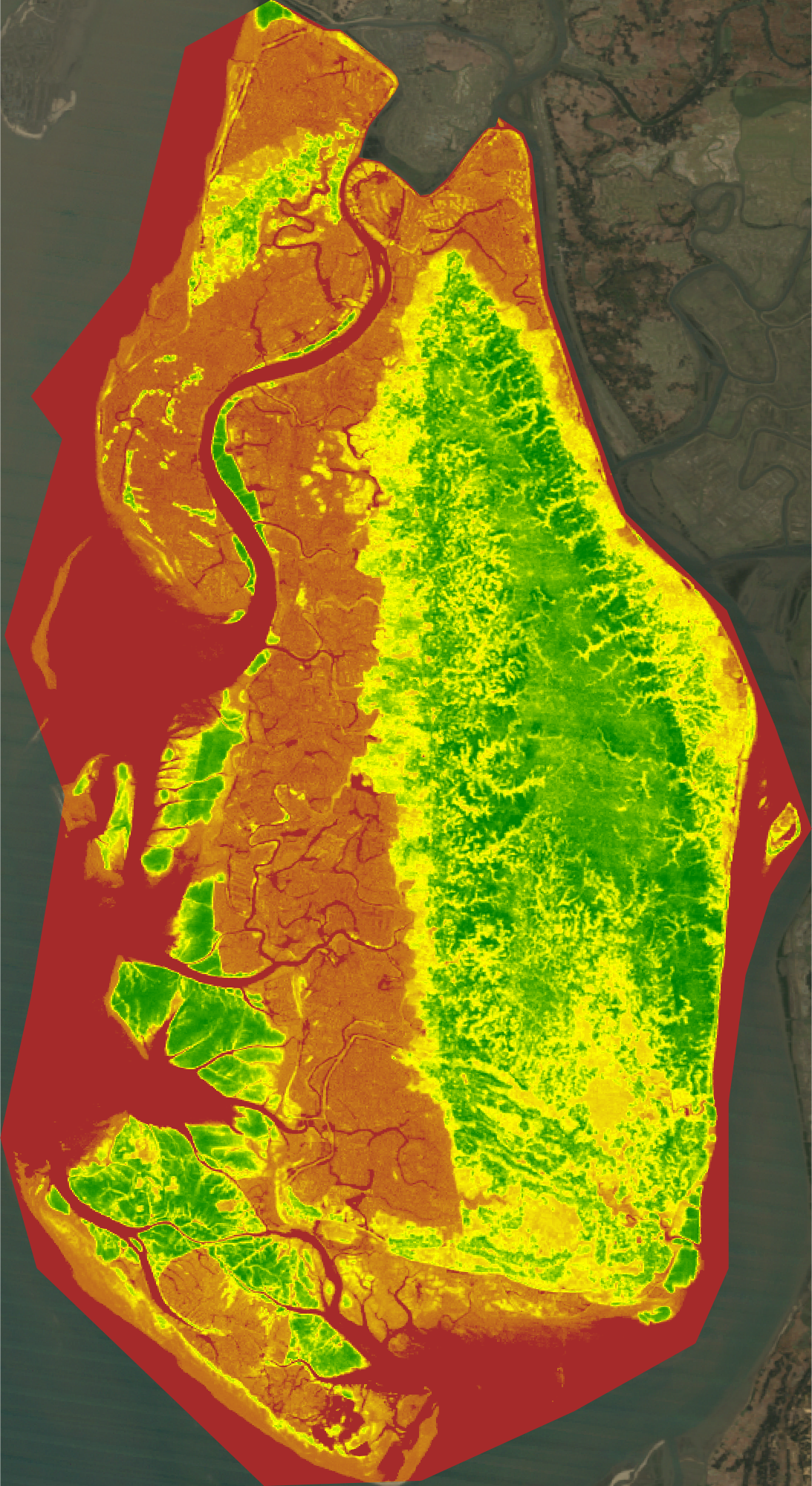
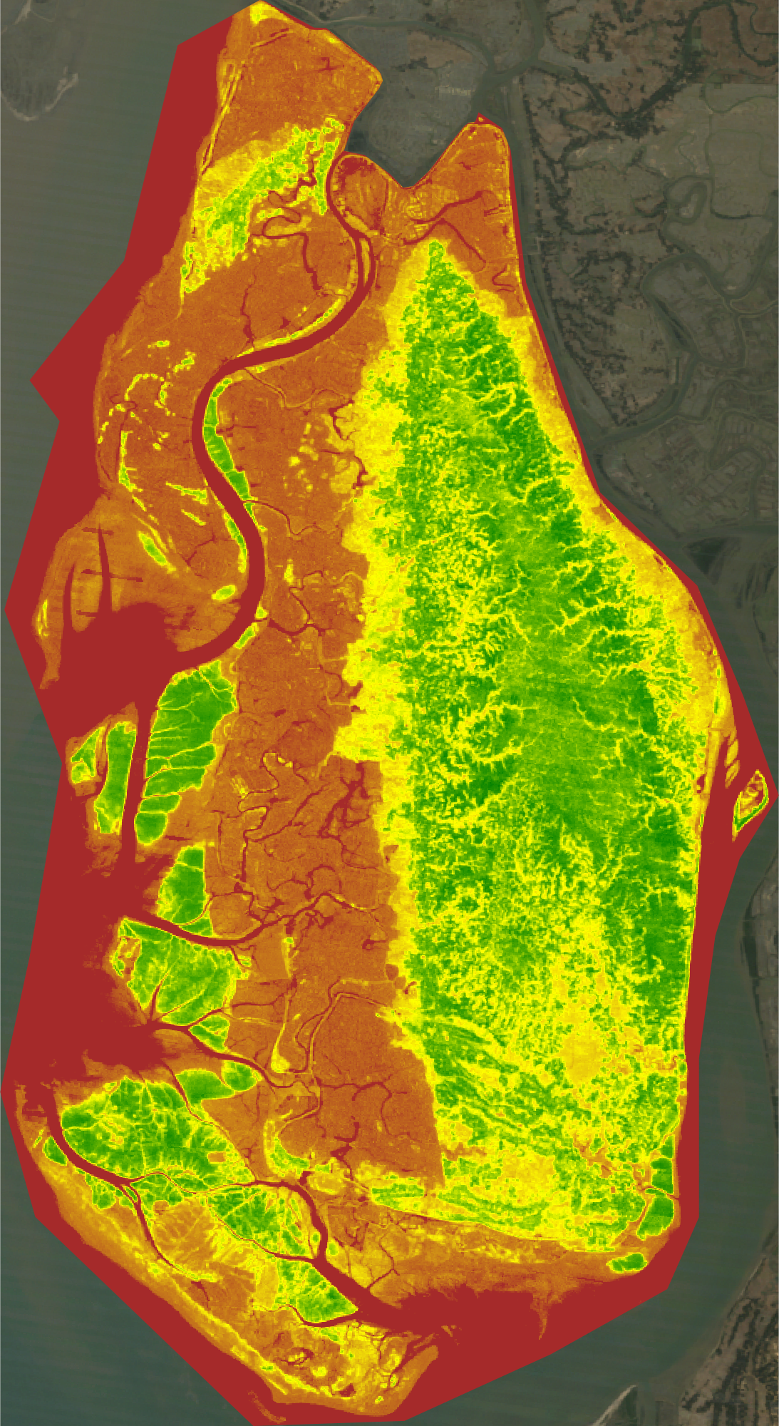
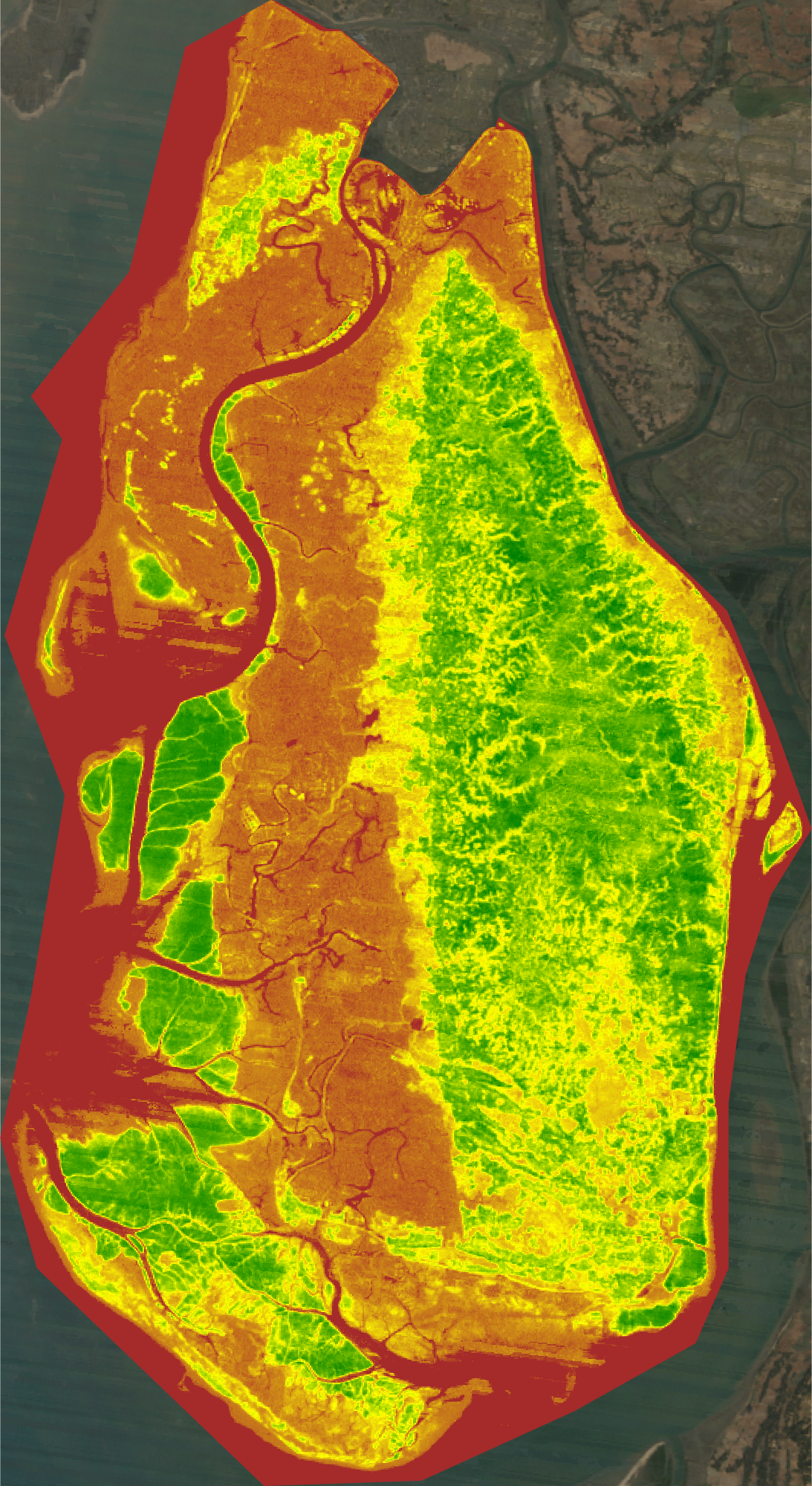
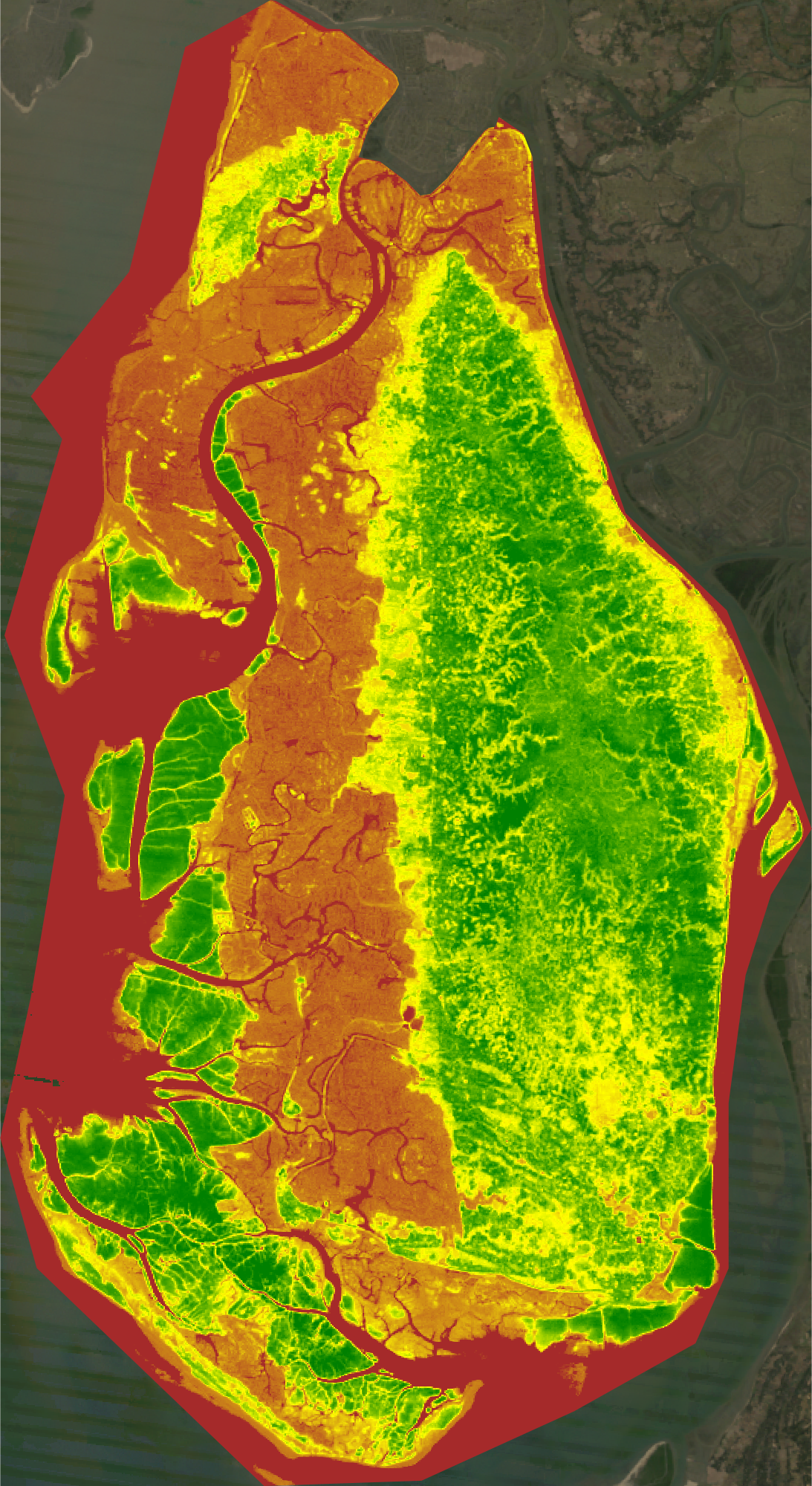
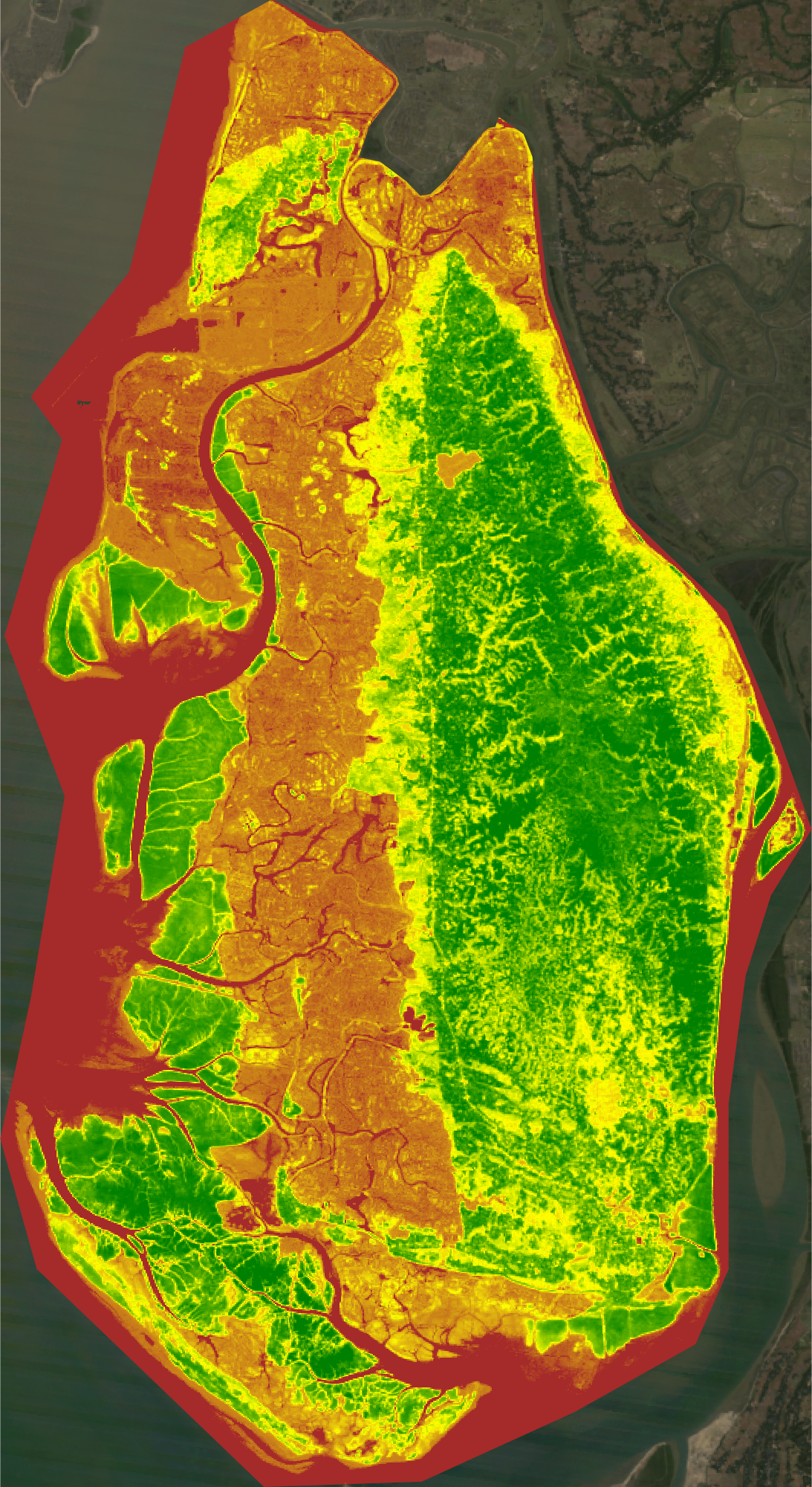
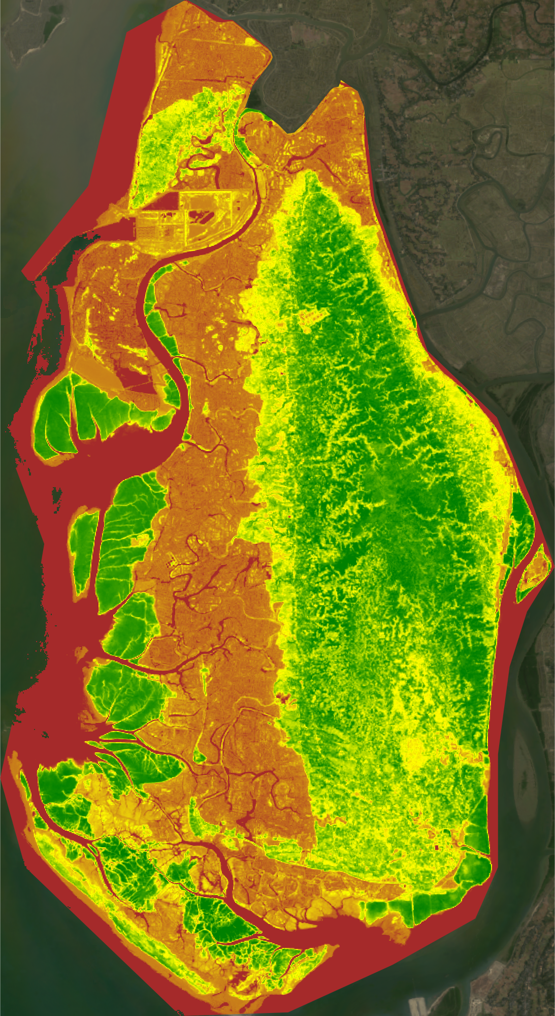
^{Figure 2 | NDVI map of Maheshkhali Upazila every 4 years from 2004 (top left) to 2024 (bottom right).In the maps, the greener an area is, the higher its NDVI. Note the changes in vegetation along the western and south-western coast over time, and the overall increase in greenness on the eastern side of the island} 

NDVI values, separated by Landsat satellites, show differences between the trends for each satellite that can be observed above (Figure 3). Confidence bands for the Landsat 8 and 9 trends are wide and encompass a zero slope, consistent with their low R² and non-significant p-values (Appendix Table 1).

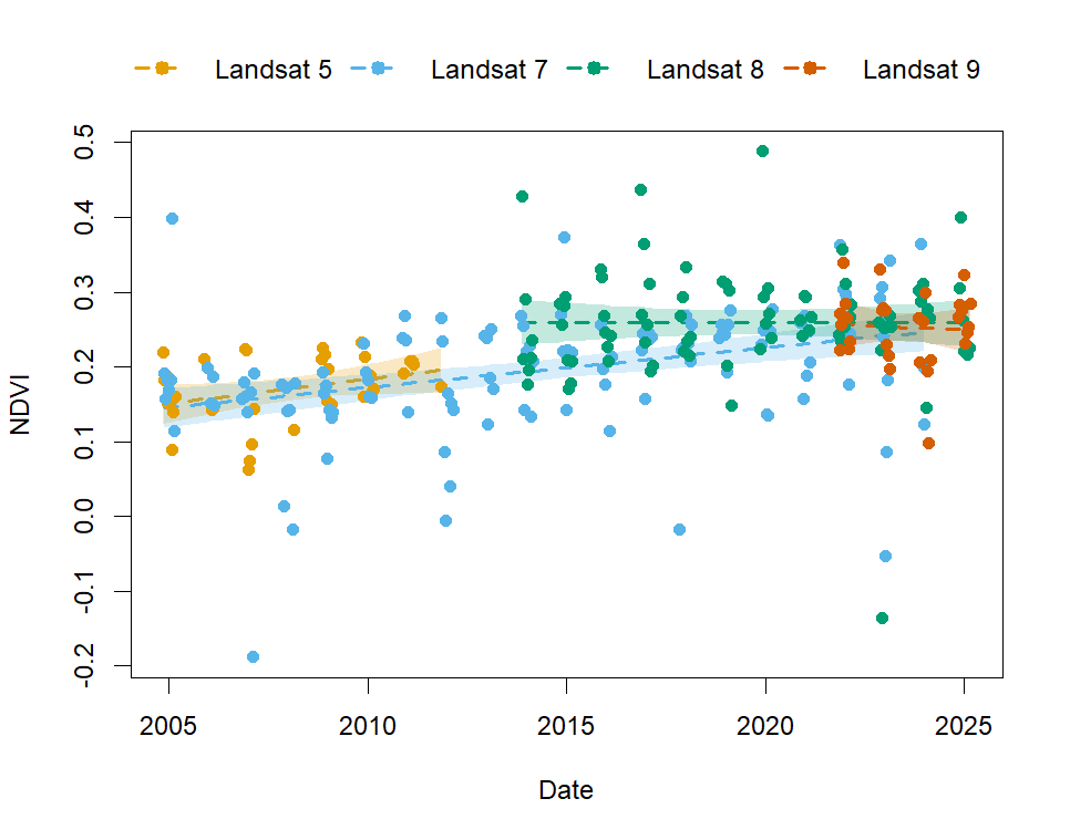
It can be seen that Landsat 8 and Landsat 9, both new satellites, appear to show decrease in NDVI, whereas Landsat 5 and Landsat 7 show an increase in NDVI (Figures 3 & 4). The 95% confidence interval for each sensor, represented by the error bars, shows that the Landsat 5 and 7 were positive, whereas Landsat 8 and 9 confidence intervals span zero, indicating slopes that are not statistically distinguishable from no change.

Visual assessment of the supervised classification outputs suggests that the area of Built-up, Agriculture, and Aquaculture has been increasing, whereas the Forest area is decreasing (Figure 5).

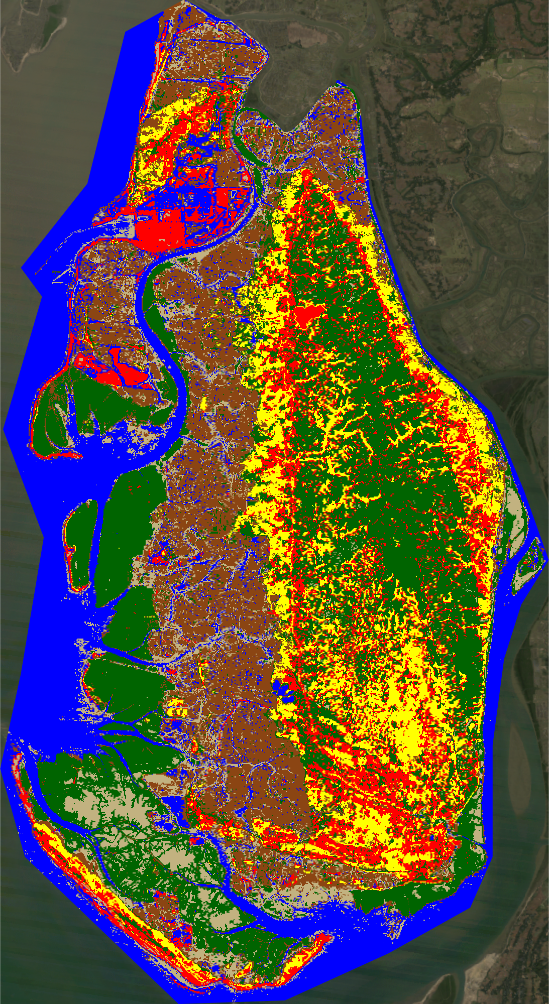
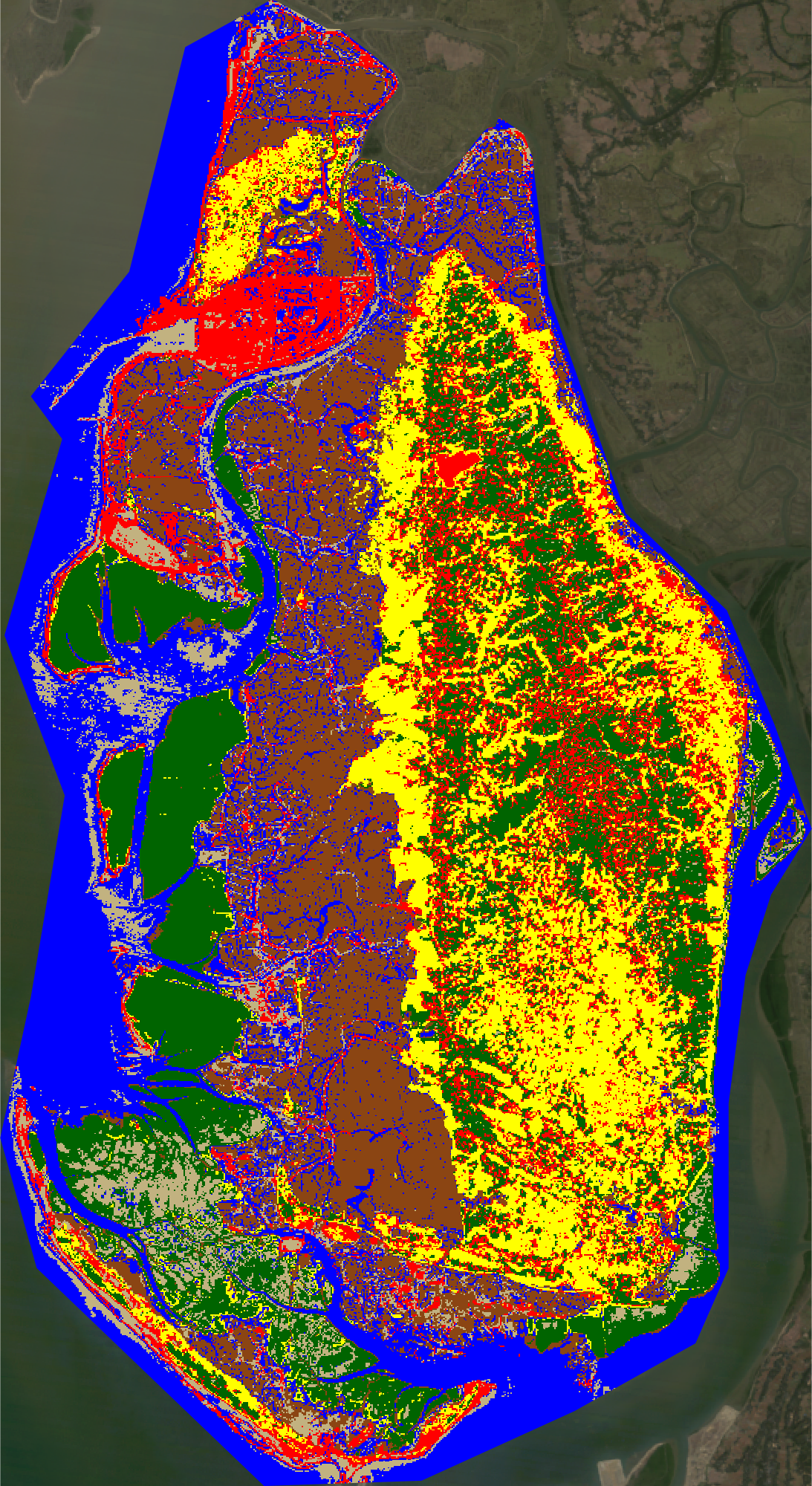
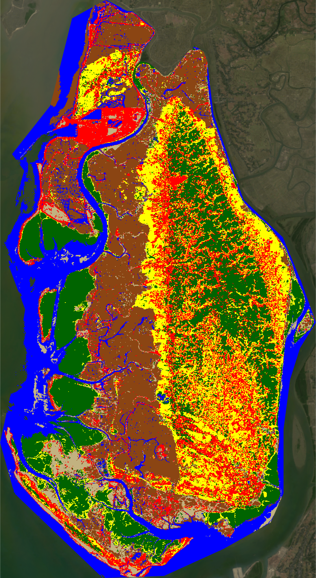
^{Figure 5 | Land Use Land Cover map of the Area of Interest (Maheshkhali Upazila) based on the 6 classes for the years 2020, 2022, and 2024 (from left to right). Note the contraction of forest (dark green) and expansion of aquaculture, agriculture, and built-up classes across the three years.} 

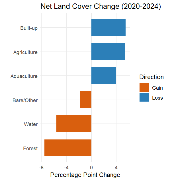
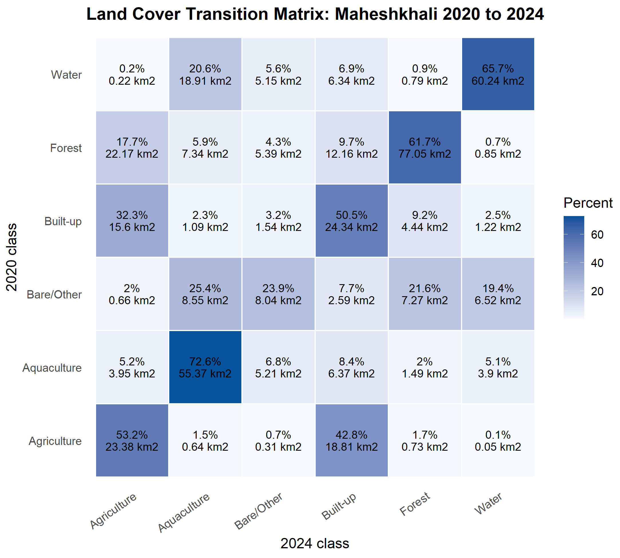
Based on the supervised classification, all classes exhibited changes in area between 2020 and 2024 (Figure 5, Figure 6, Figure 7, Figure 8). The largest change was observed in the ‘Forest (0)’ class (Figure 7, Appendix Table 2). After area adjustment (Olofsson et al., 2014), forest area was estimated at 113.9 km² in 2020 and 103.3 km² in 2024, corresponding to a forest loss of 10.7 km² (95% CI: −3.6 to +24.9 km²). This is substantially smaller than the unadjusted classification estimate of 29.17 km², and the confidence interval marginally includes zero, indicating a probable but not statistically significant decline (Appendix Table 7). Analysis of class transitions showed that, of the total forest area in 2020, 17.7% was converted to Agriculture, 5.9% to Aquaculture, 9.7% to Built-up land, 4.3% to Bare/Other land, and 0.7% to Water (Figure 8). However, these results should be interpreted with caution because the accuracy for some classes, e.g., Bare/Other (4), is lower, and the magnitude of change for them is even less reliable. From the independent validation, Producer’s Accuracy ranged from 0.32 to 0.91 and User’s Accuracy from 0.35 to 0.95 across classes, with area-adjusted overall accuracies of 0.70 (2020) and 0.74 (2024) (Appendix Table 6). These are substantially lower than the internal 70/30 figures (Appendix Table 3), most markedly for Built-up (User’s Accuracy 0.93 internally versus 0.35–0.38 independently), illustrating how non-independent validation can overstate classifier performance. 

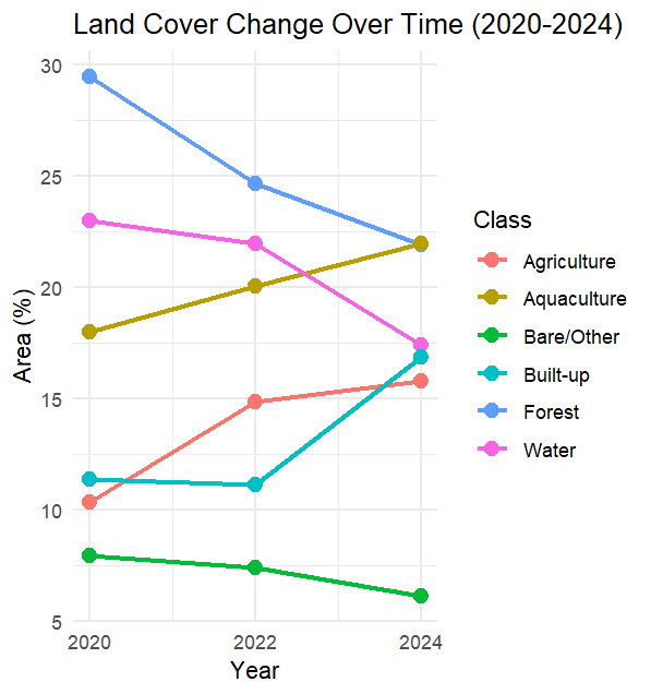
The Friedman test found no significant difference in class area percentages across the three years (χ² = 0.33, df = 2, p = 0.85). Friedman tests on producer’s and user’s accuracy were also non-significant (p = 0.31 and p = 0.51). Due to only six classes and three time points, the Friedman test has limited power.

Discussion

The NDVI maps of the island (Figure 2) show a change in LULC classes with high vegetation, i.e., Agriculture and Forest, and an increase in the greenness of the map over time can also be observed, which indicates an increase in NDVI. The increase in NDVI could be a result of multiple LULC changes, for example, reforestation, agricultural expansion, or some combination of both or some other reason altogether. The NDVI trend plots (Figures 3 & 4) reduce the necessity to depend on the visual assessment. NDVI trends, separated by Landsat satellites vary largely, where the newer satellites (Landsat 8 and 9) show a decrease in NDVI over time compared to an increase depicted by the older satellites (Landsat 5 and 7) (Figures 3 & 4). However, the apparent NDVI decline in the newer sensors is not statistically supported, and the divergence between older and newer Landsat sensors likely reflects cross-sensor differences rather than a genuine vegetation trend¹⁹. 

The NDVI data from 2004 to 2024, a much longer period than the supervised classification data, was used to get a broader range of data, which showed more explicitly the limitations of NDVI in determining forest area change. The increase in NDVI is particularly interesting since reports indicate widespread deforestation on the island ³³. This suggests that agricultural and aquacultural expansions are major drivers in the NDVI increase during the period. However, the statistical fits for the NDVI trends are weak (Appendix Table 1). Hence, the decreasing trends by sensor are not statistically supported. Also, the study did not incorporate rainfall data, and since NDVI in the region is rainfall sensitive, some of the NDVI variation could be due to interannual climate variability rather than land-cover change. Another major limitation is that cross-sensor harmonization was not done, which deems the cross-sensor trend unfit for use. When aquacultural and agricultural areas expanded, a decrease in forest area between the years 2020 and 2024 was observed from the supervised classification analysis. 

Due to the limitations of NDVI in heterogeneous islands, multi-sensor contexts, and climatic variabilities, and the weakness of the statistical fits, supervised classification for the recent years, i.e., 2020, 2022, and 2024, was done to see the actual change in LULC classes (Figure 5). The supervised classification indicated a reduction in forest area (29.17 km² unadjusted) (Appendix Table 2, Figure 7); however, once corrected for classification error using area-adjusted estimation, the forest loss was estimated at 10.7 km² (95% CI: −3.6 to +24.9 km²), considerably smaller than the unadjusted figure of 29.17 km². Because the confidence interval marginally includes zero, this result should be interpreted as a probable but not statistically confirmed forest decline. The direction of change, together with the observed class transitions and independent reporting of encroachment in the region, is consistent with ongoing forest conversion; however, the magnitude cannot be stated precisely at this spatial resolution and sampling intensity. This contrast between the raw and area-adjusted estimates highlights that unadjusted classification areas can substantially overstate land-cover change on heterogeneous coastal landscapes. The agricultural area has also increased, which may partially explain the increase in NDVI despite deforestation. The Bare/Other class had the lowest producer’s accuracy of any class in the independent validation (0.32 in 2020 and 0.37 in 2024; Appendix Table 6), meaning a large proportion of true Bare/Other pixels were not detected by the classifier⁴⁸. The apparent decrease in this class should therefore be treated with particular caution, as its magnitude and even direction are uncertain, and it is not treated as a substantive finding. It is suggested from the analysis that using NDVI trends for LULC change in a multi-sensor context and a heterogeneous island like Maheshkhali can lead to incorrect conclusions, which is also supported by previous literature¹⁶.  

This study provides evidence consistent with forest loss in Maheshkhali Upazila and points to agricultural, aquacultural, and built-up expansion as likely drivers. However, several uncertainties temper these findings. Although relying solely on NDVI trends made it difficult to conclude, using random forest-based supervised classification helped identify the trend in LULC change for each class. Hence, in the end, the effective LULC change was only interpreted for the years 2020 to 2024. This study demonstrates that in contexts of heterogeneous coastal islands like Maheshkhali, NDVI trends alone cannot fully capture the true change in forest area. However, the pairing of NDVI data with supervised classification based on the random forest method yields interpretable results. The results should therefore be read as indicative of a deforestation trend consistent with independent reporting, rather than as a definitive quantification of forest loss. The LULC maps produced can be used in future research as a baseline dataset to depict change in LULC classes.

Uncertainty is present in the long-term NDVI trend created due to differences between sensors’ different spectral band characteristics, radiometric calibration, and detector design ¹⁸, which undermined the accuracy of NDVI trends. There is also uncertainty associated with the supervised classification, as the absence of ground-truth data limited the ability to rigorously train and validate the classifier. Ground-truth validation would solidify the accuracy of the study even more, but that possibility was ruled out due to a lack of resources and logistical constraints. On top of that, only dry-season imagery has been analyzed, and although it reduces phenological noise and cloud, it does not capture seasonal cropping and aquaculture cycles during the wet season. The specific loss in the mangrove forest area vs other types of forests could not be identified due to the limitations of the classification tool, and all types of forests have been classified as one class. A low producer’s accuracy for Bare/Other (4) class also suggests that the change in bare area is less likely to be correct compared to other classes, leaving possibilities of an even increase in an area over time. The restriction of supervised classification to only 2020, 2022, and 2024, instead of the full study period, limited the temporal scope of LULC change analysis. The transition matrix was produced from a pixel-level overlay of independently trained per-year classifiers, which introduced interannual inconsistency⁴⁷. The difference between the gross forest loss shown in the transition matrix and the net loss in Table 2 arises because some pixels were classified as forest gains, largely reflecting interannual classifier inconsistency rather than genuine regrowth. Also, the net area change figures in Table 2 give a more accurate quantitative measure of forest loss, even though the transition matrix gives an idea of what percentage of the lost forest area is going to what land class, i.e., direction.

Future studies should do supervised classification of the full study period for a complete analysis of LULC change. The complementary classes should be investigated more, i.e., how the change in the area of forest relates to the change in Agriculture, and how the change in the area of water relates to the change in bare lands or aquaculture. Furthermore, the possibility of splitting the island into eastern and western halves, and separating Mangrove and Hilly forests as different classes, can be considered to better analyze and study the changes in aquaculture (western part), and Agriculture and Built-up lands (western part), as well as specific changes in mangrove or hilly forests instead of the forest area as a whole^23,31. Rainfall data should also be incorporated to reduce the uncertainties due to climate-driven NDVI variability and get more accurate, genuine vegetation change data using NDVI trends, given the strong effect of rainfall in South Asian studies¹¹.

This study provides evidence consistent with a probable decline in forest area on Maheshkhali Upazila, driven by expansion of aquaculture, agriculture, and built-up land. However, the area-adjusted analysis shows this loss is smaller and less certain than the raw classification suggests, and it does not reach statistical significance at the sampling intensity and resolution used here. The findings should therefore be read as indicative rather than definitive. The study demonstrates that NDVI analysis combined with supervised classification helps in distinguishing sensor artifacts from genuine ecosystem change. While the findings suggest a need for aquaculture zoning and enforcement of existing protections for coastal forests, such recommendations rest only on a three-year classification with broad land-cover classes and should be treated as preliminary. Firmer, spatially targeted management guidance would require denser temporal sampling and finer forest-type classes (e.g., separating mangrove from hill forest). The consequences of the loss of coastal forest area in Bangladesh are far-reaching for shoreline stability and climate resilience, and satellite-based monitoring of coastal LULC change is necessary for effective coastal governance and policymaking.

Acknowledgements

I gratefully acknowledge the United States Geological Survey (USGS) for providing Landsat data, Google Earth and Google Earth Pro for high-resolution historical satellite imagery used for independent validation, and Google Earth Engine for enabling access to and processing of the satellite imagery used in this study. I would also like to extend my sincere gratitude to Sahra Kurt, who helped me with the research for this paper. 

Data Availability

All data and code required to reproduce the analyses in this study are openly available on Zenodo at https://doi.org/10.5281/zenodo.21539696 . The repository includes the Google Earth Engine classification scripts, the R analysis scripts (NDVI trend analysis, land-cover area statistics, area-adjusted accuracy assessment, and transition analysis), the study area boundary and training polygons as shapefiles, and the independent validation datasets. The Google Earth Engine assets referenced in the scripts (study area boundary and per-year training tables) are publicly shared, and their asset paths are provided within the scripts.

Appendix

Satellite	Slope_per_year	R2	p_value
Landsat 5	0.00649	0.0995	0.0649
Landsat 7	0.00532	0.1335	0.0000
Landsat 8	-0.00011	0.0000	0.9628
Landsat 9	-0.00239	0.0035	0.7560

LULC Class	2020 (%)	2020 (km²)	2022 (%)	2022 (km²)	2024 (%)	2024 (km²)	Change 2020-24 (%)	Change 2020-24 (km²)
Forest (0)	29.43	114.32	24.62	95.64	21.92	85.15	-7.51	-29.17
Water (1)	22.97	89.22	21.93	85.18	17.39	67.55	-5.58	-21.67
Aquaculture (5)	17.97	69.80	20.02	77.78	21.94	85.23	+3.97	+15.43
Built-up (2)	11.36	44.13	11.13	43.24	16.87	65.53	+5.51	+21.40
Agriculture (3)	10.34	40.16	14.87	57.76	15.76	61.22	+5.42	+21.06
Bare/Other (4)	7.93	30.80	7.43	28.86	6.12	23.78	-1.81	-7.02

Note: Areas are unadjusted pixel-count estimates. Area-adjusted forest estimates with confidence intervals are given in Appendix Table 7 and supersede the forest figures shown here. 

Class	Producer’s	Accuracy	(Recall)	User’s	Accuracy	(Precision)
	2020	2022	2024	2020	2022	2024
Forest (0)	0.758	0.853	0.842	0.781	0.806	1.000
Water (1)	0.862	0.924	0.855	0.902	0.952	0.979
Built-up (2)	0.976	0.973	0.979	0.934	0.964	0.930
Agriculture (3)	0.852	0.930	0.718	0.885	0.816	0.875
Bare/Other (4)	0.481	0.643	0.759	0.812	0.871	0.815
Aquaculture (5)	0.855	0.886	0.844	0.783	0.775	0.818
Overall Accuracy	0.899	0.925	0.920

Map \ Reference	Forest	Water	Built-up	Agriculture	Bare/Other	Aquaculture	Total
Forest (0)	272	14	0	22	8	14	330
Water (1)	0	17	0	0	1	7	25
Built-up (2)	8	2	14	8	7	1	40
Agriculture (3)	1	0	1	36	1	1	40
Bare/Other (4)	8	4	2	0	9	2	25
Aquaculture (5)	0	3	0	1	5	31	40
Total	289	40	17	67	31	56	500

Map \ Reference	Forest	Water	Built-up	Agriculture	Bare/Other	Aquaculture	Total
Forest (0)	314	1	4	6	4	1	330
Water (1)	0	23	0	0	2	0	25
Built-up (2)	4	3	15	12	4	2	40
Agriculture (3)	9	1	1	27	2	0	40
Bare/Other (4)	2	5	0	0	15	3	25
Aquaculture (5)	0	4	1	0	4	31	40
Total	329	37	21	45	31	37	500

Class	n (2020)	n (2024)	PA 2020	UA 2020	PA 2024	UA 2024
Forest (0)	330	330	0.83	0.82	0.78	0.95
Water (1)	25	25	0.78	0.68	0.76	0.92
Built-up (2)	40	40	0.82	0.35	0.84	0.38
Agriculture (3)	40	40	0.67	0.90	0.66	0.68
Bare/Other (4)	25	25	0.32	0.36	0.37	0.60
Aquaculture (5)	40	40	0.61	0.78	0.91	0.78
Overall accuracy	500	500		0.70		0.74

PA = Producer’s Accuracy (recall); UA = User’s Accuracy (precision). Overall accuracy is the area-adjusted overall accuracy.

Estimate	Area (km²)	95% CI (km²)
Forest 2020 (area-adjusted)	113.92	104.4 to 123.4
Forest 2024 (area-adjusted)	103.26	92.6 to 113.9
Forest loss 2020–2024 (area-adjusted)	10.66	-3.6 to 24.9
Forest loss 2020–2024 (unadjusted)	29.17

Class	Polygons 2020	Pixels 2020	Polygons 2022	Pixels 2022	Polygons 2024	Pixels 2024
Forest (0)	21	90	22	90	17	70
Water (1)	42	635	37	570	32	180
Built-up (2)	36	1158	35	1099	28	1091
Agriculture (3)	23	69	33	125	35	131
Bare/Other (4)	28	152	28	157	25	148
Aquaculture (5)	24	229	18	112	16	97
Total	175	2333	172	2153	153	1717

Note: No class-balancing was applied. Polygon counts are derived from the training feature lists in the Google Earth Engine scripts. Pixel counts are the samples extracted at 30 m resolution using sampleRegions.

References

1. S. A. Adegboyega, J. Oloukoi, A. E. Olajuyigbe, O. E. Ajibade. Evaluation of unsustainable land use/land cover change on ecosystem services in coastal area of lagos state, nigeria. Applied Geomatics. Vol. 11, pg. 97–110, 2019 https://doi.org/10.1007/s12518-018-0242-2 [↩]
2. D. A. Friess, K. Rogers, C. E. Lovelock, K. W. Krauss, S. E. Hamilton, S. Y. Lee, R. Lucas, J. Primavera, A. Rajkaran, S. Shi. The state of the world’s mangrove forests: past, present, and future. Annual Review of Environment and Resources. Vol. 44, pg. 89–115, 2019 https://doi.org/10.1146/annurev-environ-101718-033302 [↩] [↩]
3. M. F. Adame, R. M. Connolly, M. P. Turschwell, C. E. Lovelock, T. Fatoyinbo, D. Lagomasino, L. A. Goldberg, J. Holdorf, D. A. Friess, S. D. Sasmito, J. Sanderman, M. Sievers, C. Buelow, J. B. Kauffman, D. Bryan-Brown, C. J. Brown. Future carbon emissions from global mangrove forest loss. Global Change Biology. Vol. 27, pg. 2856–2866, 2021 https://doi.org/10.1111/gcb.15571 [↩]
4. S. L. Goodbred, S. A. Kuehl. The significance of large sediment supply, active tectonism, and eustasy on margin sequence development: late quaternary stratigraphy and evolution of the ganges–brahmaputra delta. Sedimentary Geology. Vol. 133, pg. 227–248, 2000 https://doi.org/10.1016/S0037-0738(00)00041-5 [↩]
5. S. Parvin, Md. H. Sakib, Md. L. Islam, C. L. Brown, Md. S. Islam, Y. Mahmud. Coastal aquaculture in bangladesh: sundarbans’s role against climate change. Marine Pollution Bulletin. Vol. 194, pg. 115431, 2023 https://doi.org/10.1016/j.marpolbul.2023.115431 [↩] [↩]
6. X. Xu, D. Fu, F. Su, V. Lyne, H. Yu, J. Tang, X. Hong, J. Wang. Global distribution and decline of mangrove coastal protection extends far beyond area loss. Nature Communications. Vol. 15, pg. 10267, 2024 https://doi.org/10.1038/s41467-024-54349-0 [↩]
7. V. Hagger, T. A. Worthington, C. E. Lovelock, M. F. Adame, T. Amano, B. M. Brown, D. A. Friess, E. Landis, P. J. Mumby, T. H. Morrison, K. R. O’Brien, K. A. Wilson, C. Zganjar, M. I. Saunders. Drivers of global mangrove loss and gain in social-ecological systems. Nature Communications. Vol. 13, pg. 6373, 2022 https://doi.org/10.1038/s41467-022-33962-x [↩] [↩]
8. M. K. Islam, M. Hasan, M. Rahman, R. Fayyaz, M. Chowdhury, T. Hamid. Shoreline dynamics assessment of moheshkhali island of bangladesh using integrated gis-dsas techniques. The Dhaka University Journal of Earth and Environmental Sciences. Vol. 11, pg. 1–14, 2022 https://doi.org/10.3329/dujees.v11i1.63707 [↩] [↩]
9. A. Khan Majlis, M. Islam, M. Khasru, M. Ahsan. Protected to open basin depositional system: an appraisal for the late quaternary evolution of the moheshkhali-kutubdia coastal plain, bangladesh. Bangladesh Journal of Geology. Vol. 26, pg. 16–28, 2013 [↩]
10. Md. M. H. Saddam, K. T. Hossain, P. Mollick, Md. Salauddin, S. Roy, A. U. Ahmad, R. C. Bhowmick, Md. A. I. Rony. Shoreline dynamics in response to sea-level changes on the eastern coast of bangladesh. Environmental Monitoring and Assessment. Vol. 197, pg. 942, 2025 https://doi.org/10.1007/s10661-025-14375-x [↩] [↩]
11. G. Rahman, U. Farooq, M.-K. Jung, H.-H. Kwon. Spatiotemporal vegetation dynamics in south asia (2001-2023): roles of climate and anthropogenic activities. Geoscience Letters. Vol. 12, pg. 31, 2025 https://doi.org/10.1186/s40562-025-00403-8 [↩] [↩] [↩]
12. Md. R. Islam, Md. Esraz-Ul-Zannat. Remote sensing based investigation of coastal lulc dynamics in the coastal region of bangladesh. Remote Sensing Applications: Society and Environment. Vol. 31, pg. 100982, 2023 https://doi.org/10.1016/j.rsase.2023.100982 [↩]
13. Landsat Missions. Landsat normalized difference vegetation index. U.S. Geological Survey https://www.usgs.gov/landsat-missions/landsat-normalized-difference-vegetation-index 2025 [↩]
14. L. Ruan, M. Yan, L. Zhang, X. Fan, H. Yang. Spatial-temporal ndvi pattern of global mangroves: a growing trend during 2000-2018. The Science of the Total Environment. Vol. 844, pg. 157075, 2022 https://doi.org/10.1016/j.scitotenv.2022.157075 [↩]
15. R. Kumar, A. J. Nath, A. Nath, N. Sahu, R. Pandey. Landsat-based multi-decadal spatio-temporal assessment of the vegetation greening and browning trend in the eastern indian himalayan region. Remote Sensing Applications: Society and Environment. Vol. 25, pg. 100695, 2022 https://doi.org/10.1016/j.rsase.2022.100695 [↩] [↩]
16. A. Nițu, C. Florea, M. Ivanovici, A. Racoviteanu. NDVI and beyond: vegetation indices as features for crop recognition and segmentation in hyperspectral data. Sensors. Vol. 25, pg. 3817, 2025 https://doi.org/10.3390/s25123817 [↩] [↩] [↩]
17. G. T. Yengoh, D. Dent, L. Olsson, A. E. Tengberg, C. J. Tucker Iii. Use of the Normalized Difference Vegetation Index (NDVI) to assess land degradation at multiple scales: current status, future trends, and practical considerations. Springer International Publishing, Cham, 2016 https://doi.org/10.1007/978-3-319-24112-8 [↩]
18. D. P. Roy, V. Kovalskyy, H. K. Zhang, E. F. Vermote, L. Yan, S. S. Kumar, A. Egorov. Characterization of landsat-7 to landsat-8 reflective wavelength and normalized difference vegetation index continuity. Remote Sensing of Environment. Vol. 185, pg. 57–70, 2016 https://doi.org/10.1016/j.rse.2015.12.024 [↩] [↩]
19. G. Mancino, A. Ferrara, A. Padula, A. Nolè. Cross-comparison between landsat 8 (oli) and landsat 7 (etm+) derived vegetation indices in a mediterranean environment. Remote Sensing. Vol. 12, pg. 291, 2020 https://doi.org/10.3390/rs12020291 [↩] [↩]
20. M. Wu, Z. Huang, S. Liu, Z. Wu, T. Hong, X. Hu. Vegetation-cover change trends across different lengths of time series using ndvi: contrasting theil–sen and mann–kendall with piece-wise regression. Forests. Vol. 17, pg. 557, 2026 https://doi.org/10.3390/f17050557 [↩]
21. J. Sun, S. Ongsomwang. Optimal parameters of random forest for land cover classification with suitable data type and dataset on google earth engine. Frontiers in Earth Science. Vol. 11, pg. 1188093, 2023 https://doi.org/10.3389/feart.2023.1188093 [↩] [↩]
22. S. Praticò, F. Solano, S. Di Fazio, G. Modica. Machine learning classification of mediterranean forest habitats in google earth engine based on seasonal sentinel-2 time-series and input image composition optimisation. Remote Sensing. Vol. 13, pg. 586, 2021 https://doi.org/10.3390/rs13040586 [↩] [↩] [↩] [↩]
23. A. Ghorbanian, S. Zaghian, R. M. Asiyabi, M. Amani, A. Mohammadzadeh, S. Jamali. Mangrove ecosystem mapping using sentinel-1 and sentinel-2 satellite images and random forest algorithm in google earth engine. Remote Sensing. Vol. 13, pg. 2565, 2021 https://doi.org/10.3390/rs13132565 [↩] [↩]
24. M. Belgiu, L. Drăguţ. Random forest in remote sensing: a review of applications and future directions. ISPRS Journal of Photogrammetry and Remote Sensing. Vol. 114, pg. 24–31, 2016 https://doi.org/10.1016/j.isprsjprs.2016.01.011 [↩]
25. X. Yan, J. Li, A. R. Smith, D. Yang, T. Ma, Y. Su. Rapid land cover classification using a 36-year time series of multi-source remote sensing data. Land. Vol. 12, pg. 2149, 2023 https://doi.org/10.3390/land12122149 [↩]
26. T. N. Phan, V. Kuch, L. W. Lehnert. Land cover classification using google earth engine and random forest classifier—the role of image composition. Remote Sensing. Vol. 12, pg. 2411, 2020 https://doi.org/10.3390/rs12152411 [↩]
27. S. M. Nazmul Haque, M. J. Uddin. Monitoring lulc dynamics and detecting transformation hotspots in sylhet, bangladesh (2000–2023) using google earth engine. Scientific Reports. Vol. 15, pg. 31263, 2025 https://doi.org/10.1038/s41598-025-07443-2 [↩]
28. A. Fallatah, A. Alattas, A. Habibullah, A. Mandourah, R. Sahahiri, A. Baik, Y. Alshawabkeh, M. Elfleet. Monitoring mangrove deforestation using google earth engine and random forest machine learning algorithm. Land. Vol. 15, pg. 901, 2026 https://doi.org/10.3390/land15060901 [↩]
29. Rahman, A. Ceanturi, J. W. Tuahatu, F. F. Lokollo, J. Supusepa, M. Hulopi, Y. I. Permatahati, Y. A. Lewerissa, Y. Wardiatno. Mangrove ecosystems in southeast asia region: mangrove extent, blue carbon potential and co2 emissions in 1996–2020. Science of The Total Environment. Vol. 915, pg. 170052, 2024 https://doi.org/10.1016/j.scitotenv.2024.170052 [↩]
30. A. Ahmed, F. Drake, N. Nawaz, C. Woulds. Where is the coast? monitoring coastal land dynamics in bangladesh: an integrated management approach using gis and remote sensing techniques. Ocean and Coastal Management. Vol. 151, pg. 10–24, 2017 https://doi.org/10.1016/j.ocecoaman.2017.10.030 [↩] [↩]
31. Z. Zhang, M. R. Ahmed, Q. Zhang, Y. Li, Y. Li. Monitoring of 35-year mangrove wetland change dynamics and agents in the sundarbans using temporal consistency checking. Remote Sensing. Vol. 15, pg. 625, 2023 https://doi.org/10.3390/rs15030625 [↩] [↩]
32. S. Samanta, S. Hazra, P. P. Mondal, A. Chanda, S. Giri, J. R. French, R. J. Nicholls. Assessment and attribution of mangrove forest changes in the indian sundarbans from 2000 to 2020. Remote Sensing. Vol. 13, pg. 4957, 2021 https://doi.org/10.3390/rs13244957 [↩]
33. S. Newase, M. R. Acharjee, A. Talukder, S. Q. Nishi. Temporal evolution of land use-land cover changes, focusing on present mariculture sites along the moheshkhali island, bangladesh. GeoJournal. Vol. 89, pg. 54, 2024 https://doi.org/10.1007/s10708-024-11060-3 [↩] [↩] [↩]
34. M. Govender, J. Das, S. Paul, S. S. Shuvo, S. A. Selim, M. Glaser. Toward blue justice in blue growth: insights from local discourses on coastal megaprojects in bangladesh. Ocean & Coastal Management. Vol. 269, pg. 107766, 2025 https://doi.org/10.1016/j.ocecoaman.2025.107766 [↩]
35. P. K. Bellam, M. K. Gumma, P. Panjala, I. Mohammed, A. Suzuki. Mapping shrimp pond dynamics: a spatiotemporal study using remote sensing data and machine learning. AgriEngineering. Vol. 5, pg. 1432–1447, 2023 https://doi.org/10.3390/agriengineering5030089 [↩]
36. Md. M. Morshed, Md. S. Islam, H. D. Lohano, P. Shyamsundar. Production externalities of shrimp aquaculture on paddy farming in coastal bangladesh. Agricultural Water Management. Vol. 238, pg. 106213, 2020 https://doi.org/10.1016/j.agwat.2020.106213 [↩]
37. M. E. Hasan, L. Zhang, R. Mahmood, H. Guo, G. Li. Modeling of forest ecosystem degradation due to anthropogenic stress: the case of rohingya influx into the cox’s bazar–teknaf peninsula of bangladesh. Environments. Vol. 8, pg. 121, 2021 https://doi.org/10.3390/environments8110121 [↩]
38. M. Rahaman, M. M. Morshed, S. Bhadra. An integrated machine learning and remote sensing approach for monitoring forest degradation due to rohingya refugee influx in bangladesh. Remote Sensing Applications: Society and Environment. Vol. 25, pg. 100696, 2022 https://doi.org/10.1016/j.rsase.2022.100696 [↩]
39. Bangladesh Bureau of Statistics. 2024 Bangladesh statistical yearbook. Bangladesh Bureau of Statistics, 2025 [↩]
40. F. E. Onuegbu, A. U. Egbu. Employing post classification comparison to detect land use cover change patterns and quantify conversions in abakaliki lga nigeria from 2000 to 2022. Scientific Reports. Vol. 14, pg. 9384, 2024 https://doi.org/10.1038/s41598-024-59056-w [↩]
41. W. A. Bagwan, R. Sopan Gavali. Dam-triggered land use land cover change detection and comparison (transition matrix method) of urmodi river watershed of maharashtra, india: a remote sensing and gis approach. Geology, Ecology, and Landscapes. Vol. 7, pg. 189–197, 2023 https://doi.org/10.1080/24749508.2021.1952762 [↩]
42. Z. Deng, B. Quan. Intensity analysis to communicate detailed detection of land use and land cover change in chang-zhu-tan metropolitan region, china. Forests. Vol. 14, pg. 939, 2023 https://doi.org/10.3390/f14050939 [↩]
43. S. D. D. M. Deguenon, O. N. F. Baguere, O. Teka, D. W. Aheto, B. Sinsin. Using of intensity analysis approach in benin coastal zone (west africa) to assess land use/land cover change for further decision making. Heliyon. Vol. 8, pg. e12384, 2022 https://doi.org/10.1016/j.heliyon.2022.e12384 [↩]
44. Y. Wang, R. Shi, B. Zhao, S. Yang, J. Yang. Land transition intensity spectrum: a novel method for analyzing stable and systematic land use and land cover change patterns. Environmental Monitoring and Assessment. Vol. 197, pg. 1180, 2025 https://doi.org/10.1007/s10661-025-14672-5 [↩]
45. P. Olofsson, G. M. Foody, M. Herold, S. V. Stehman, C. E. Woodcock, M. A. Wulder. Good practices for estimating area and assessing accuracy of land change. Remote Sensing of Environment. Vol. 148, pg. 42–57, 2014 https://doi.org/10.1016/j.rse.2014.02.015 [↩]
46. P. Olofsson, G. M. Foody, S. V. Stehman, C. E. Woodcock. Making better use of accuracy data in land change studies: estimating accuracy and area and quantifying uncertainty using stratified estimation. Remote Sensing of Environment. Vol. 129, pg. 122–131, 2013 https://doi.org/10.1016/j.rse.2012.10.031 [↩]
47. S. V. Stehman, G. M. Foody. Key issues in rigorous accuracy assessment of land cover products. Remote Sensing of Environment. Vol. 231, pg. 111199, 2019 https://doi.org/10.1016/j.rse.2019.05.018 [↩] [↩]
48. S. V. Stehman, D. Xing. Confidence intervals for proportion of area estimated from a stratified random sample. Remote Sensing of Environment. Vol. 280, pg. 113193, 2022 https://doi.org/10.1016/j.rse.2022.113193 [↩]