Understanding AGN Evolution with Principal Component Analysis Across Varying Redshift Ranges

Abstract

The evolution of galaxy spectra with redshift is central to studies of chemical enrichment, ionization evolution, and star formation history. Many emission line diagnostics pre-select lines or line regions and use techniques calibrated to low-redshift objects, resulting in systematic errors at high redshift. We use principal component analysis (PCA) to analyze rest-frame QSO spectra from SDSS Data Release 16 (DR16) from redshifts ~0 to ~2. We apply a quality cut of median S/N > 5 to 100 spectra in five bins of width 0.4 in redshift. There are 20 spectra (n = 20) in each redshift bin. PCA is performed separately after continuum normalization and mean subtraction for each bin. PC1 accounts for approximately 24-52% of the total spectral variance and represents the strength of emission lines. PC1 scores show a correlation with observed Hα equivalent widths (Spearman ρ = 0.952, p = 1.1 x 10^-10, N = 20) in the lowest redshift bin. At low redshift, PC1 scores span a wide range, indicating much diversity in emission-line strength. At high redshift, PC1 scores span a narrower range with a positive skew; however, since each bin’s scores are projections onto a different eigenvector over a different rest-frame wavelength range, this difference in scale must not be directly interpreted as evolution in AGN strength. Bins 1 and 5 (original scores) are compared via a Kolmogorov-Smirnov test and produce results of D = 0.40, p = 0.081 (n₁ = n₅ = 20).This result is not significant at α = 0.05, and after standardizing scores to zero mean and unit variance the distributions are indistinguishable (D = 0.15, p = 0.98), indicating that the raw difference reflects score scale rather than distribution shape. Several caveats are present, such as the lack of common rest-frame wavelengths for all bins and selection effects due to QSO samples. Suggestions for future research are included.

Keywords: principal component analysis (PCA), quasar spectra, galaxy spectral evolution, redshift bins, SDSS DR16, emission lines, eigenspectra

Introduction

One of the major problems in observational astrophysics is the study of galaxy evolution. A method commonly used for this is the study of optical emission lines in the spectra of galaxies. From these lines, one can infer the physical conditions and chemical composition of the interstellar medium (ISM). Emission line fluxes and line ratios can also be used to determine gas phase metallicities^1,2,3, the strength of an active galactic nucleus (AGN)^4,5, and star formation rates⁶. Star formation increased and then decreased dramatically in the universe between the present day (z ≈ 0) and 10 billion years ago (z ≈ 2). The peak value of star formation occurred at z ≈ 1.5-2.5, or during “cosmic noon” ³ and has significantly dropped to the present. Therefore, galaxies underwent a transition from almost entirely star forming structures in the past to a bimodality of active star forming spirals and inactive elliptical galaxies today^2,7.

Regularly used emission-line evaluation methods have important limitations, however, that become especially problematic for comparative studies spanning a wide redshift baseline. Diagrams such as the Baldwin-Phillips-Terlevich (BPT) diagram⁸ need the simultaneous detection of four or more specific lines (Hα, Hβ, [O III], [N II]) as key lines redshift out of the observable optical window of wavelength at z > 0.4, so maintaining consistent line coverage becomes increasingly difficult.

Strong line metallicity calibrations from local H II regions carry systematic uncertainties of 0.2-0.4 dex and differ by non negligible amounts between other calibration techniques³; Kewley & Ellison (2008) showed that common lines (R23, O3N2, N2) give inconsistent oxygen abundances with intercept offsets of ~0.15-0.4 dex in the local mass-metallicity relation³. These calibration systematics are also seen at higher redshift^9,10 and are further worsened if ISM conditions — ionization parameter, N/O ratio, electron density — evolve between epochs.

Also, the ionization conditions of higher redshift galaxies can differ systematically from others with similar redshift: high-z star-forming galaxies lie systematically offset from the z ≈ 0 point on the BPT diagram^11,12,13, driven by harder ionizing spectra from alpha-enhanced stellar populations, higher than expected N/O ratios, higher ionization parameters, and higher gas densities^14,15.

Recent JWST/NIRSpec observations using direct electron-temperature metallicities from the [O III] λ4363 line at 2 < z < 9 have shown that standard z ≈ 0 calibrations actually underestimate gas phase oxygen abundances by up to ~1 dex when applied at z ≈ 4-8^16,17,18,19. Laseter et al. (2024) used ten [O III] λ4363 auroral detections in JADES galaxies up to z ≈ 9.5 and found that existing strong-line calibrations fail to simultaneously match the emission-line properties of their sample at these redshifts¹⁸.

These results show that applying locally calibrated emission-line methods to high z samples introduces biases large enough to hide rather than reveal genuine evolutionary trends, and motivate the search for calibration-free approaches to characterizing spectral evolution.

Principal component analysis (PCA) gives us a data driven method that tackles some of these issues. By identifying the dominant axes of spectral variance in an unsupervised manner, that is, without pre-selecting which lines or ratios to measure, PCA allows the data itself to show which spectral features vary most within a given sample. PCA has been successfully applied to SDSS galaxy spectra at low redshift (ex. Yip et al. 2004²⁰, who analyzed ~170,000 SDSS spectra and showed that a couple of eigenspectra describe the dominant spectral types; Wild et al. 2007²¹, who applied PCA to the 3750–4150 Å region of galaxy spectra and found that PC1 traces the 4000 Å break strength, a measure of recent star formation history) and to quasar spectra across redshift.

Francis et al. (1992)²² experimented with the foundational spectral PCA on 232 quasars, using wavelength bin fluxes as variables directly rather than using pre measured line parameters, thereby ridding the need to model the continuum or Fe II pseudocontinuum, similar to the calibration free pipeline our present work exercises. Yip et al. (2004)²³ continued this to 16,707 SDSS DR1 quasar spectra spanning from 0.08 < z < 5.41 and found that spectral classification itself depends on redshift and luminosity, providing the most direct experiment to the redshift binned PCA comparison here.

Pâris et al. (2011)²⁴ applied PCA to 78 high-quality SDSS DR7 quasar UV spectra at z ≈ 3, again finding a couple of eigenspectra, enough to capture dominant spectral variation.

Ma et al. (2019)²⁵ applied PCA to the 4000–5500 Å (Hβ) region of ∼10,000 low-redshift SDSS quasars and found that PC1 corresponds to the “Eigenvector 1” anticorrelation between [O III] and Fe II strengths. Suzuki (2006)²⁶ then independently showed that the first two PCs account for ~80% of variance in low z quasar samples.

To our knowledge, no previous study has applied this per-bin PCA logic to SDSS DR16 Type 1 QSO spectra spanning z ≈ 0-2 to examine how the primary mode of spectral variation evolves over cosmic time.

The analysis here does PCA to QSO spectra from the SDSS DR16 QSO catalog^27,28 divided into five redshift bins (z = 0.0-0.4, 0.4-0.8, 0.8-1.2, 1.2-1.6, and 1.6-2.0). Factors such as uniform instrument characteristics, flux calibration, and noise properties across all bins are guaranteed by sampling only from a single survey.

The main goal here is to determine what the leading spectral variance mode is in each bin, and whether that mode changes from z ≈ 2 to z ≈ 0 in ways consistent with known evolutionary trends such as the decline in cosmic star formation and the growth of passive galaxy populations. The approach is complementary to line-ratio diagnostics, as while diagnostics answer “what are the values of specific line ratios?”, PCA answers “what is the dominant way in which spectra within a sample differ from one another?”.

The scope of this study is focused – spectra are drawn exclusively from SDSS DR16, restricting the sample to Type 1 quasars from 0.0 ≤ z ≤ 2.0 ,observed with the same instrument and pipeline. The central research question is, does the dominant mode of spectral variance, as identified by PCA, change across five redshift bins spanning from z = 0-2, and if so, in a manner that lines up with known evolutionary trends in star formation and AGN activity?

This paper reviews the (relevant) background in galaxy emission lines and AGNs, describes the data and preprocessing pipeline in reproducible detail, and gives per-bin PCA results with astrophysical interpretation, and concludes with a discussion of limitations and future directions.

Prpoerties of Galaxies and Emission Lines

Emission Lines as Diagnostic Tools

When an optical spectrum of a galaxy or quasar is observed, it contains not only the starlight (the continuum) but also emission lines at specific wavelengths as a product of the hot, ionized gas. In star forming galaxies, this gas resides mostly in H II regions ionized by short lived, massive young stars. In AGN, it occupies the broad-line region (BLR) and narrow-line region (NLR) lit up by the accretion disk⁴. Different elements and ions radiate at well known rest frame wavelengths, making emission lines essential tools when searching for physical conditions in the ISM and AGN environments.

The hydrogen Balmer series gives us direct flags of ionized gas and star formation. Hα at 6563 Å is a particularly well known and obvious indicator of recent star formation⁶, coming from H II regions excited by OB stars with lifetimes of only a few million years. Additionally, Hβ at 4861 Å is frequently paired with other lines to constrain dust extinction (via the Balmer decrement Hα/Hβ) and gas temperature.

The forbidden line [O III] λ5007 Å (doubly ionized oxygen) is important when identifying high energy ionizing photons. Because its upper energy level consists by collisional excitation, [O III] is bright in low-metallicity, high-ionization states or in regions with hard ionizing radiation from AGN or extreme starbursts²⁹. The ratio [O III]/Hβ is also used ionization parameter diagnostic; high values (> 3) show AGN activity or very hot, young starbursts^8,4,5.

The forbidden line [N II] λ6583 Å lies close in wavelength to Hα, and is often used with it. The ratio [N II]/Hα increases with gas phase metallicity^30,3 and is heightened in AGN ionized gas, making it a fundamental of the BPT diagram^8,5. The BPT diagram also uses [O III]/Hβ versus [N II]/Hα to classify spectra as arising from H II regions, AGN, or composite systems.

Again, a known and recognized limitation of the diagram and of strong-line calibrations based on it is their dependence on the simultaneous detection of four emission lines and their derivation from local galaxy samples, which may not represent conditions at high redshift^11,31,3.

Additional important emission features include [O II] λ3727 Å (a singly ionized oxygen doublet used as a star-formation indicator at high redshift when Hα redshifts beyond the optical³), the sulfur doublet [S II] λ λ6716,6731 A (useful for diagnosing gas density³²), He II λ4686 A and [Ne III] λ3869 Å (tracers of very-high-energy photons capable of doubly ionizing helium or neon, signaling hard AGN ionization fields or extremely low-metallicity stellar populations). Also, absorption lines such as the Calcium H and K doublet (3934, 3969 Å), Mg I (5175 Å), and the sodium D doublet (5890, 5896 Å) trace stellar populations in passive or mildly active galaxies and appear as negative equivalent width features in the spectra.

Active Galactic Nuclei and Emission-Line Regions

An AGN is powered by accretion of matter onto a supermassive black hole and gives off intense ultraviolet and X-ray radiation that photoionizes surrounding gas⁴. AGN are broadly sorted as Type 1 (unobscured, showing both broad and narrow lines) or Type 2 (obscured, showing only narrow lines), with the distinction given by the viewing angle relative to a dusty torus in the unified AGN model⁴.

Emission lines in AGN originate in two distinct regions. The broad line region (BLR), located within ~0.01-0.1 pc of the black hole, consists of dense, rapidly orbiting gas clouds that give us broad permitted lines (such as Hα, Hβ, and Mg II) with Doppler widths of thousands of km/s⁴. These broad components are optically visible in Type 1 AGN, including the quasars analyzed in this study. The narrow-line region (NLR) extends from just outside the disk to hundreds or even thousands of parsecs away and gives us narrow forbidden and semi-forbidden lines, like [O III] λ5007, [N II] λ6583, [O II] λ3727, [S II] λ λ 6716, 6731, with widths of a few hundred km/s⁴. Both Type 1 and Type 2 AGN exhibit NLR emission, since this region is so big that a small dust ring can’t hide it entirely.

The sample we looked at in this work is entirely of spectroscopically confirmed Type 1 QSOs from SDSS DR16. As such, the AGN contribution to spectral emission isn’t just an impurity to be separated from star formation but is the planned and main source of emission line variability in the sample. The principal axes of spectral variance identified by PCA will thus show us variations in AGN activity level, continuum power law slope, BLR physics, and NLR excitation rather than star formation per se. This context is needed for interpreting PC1 scores as reflecting AGN spectral strength rather than purely stellar ionization.

Evolution of Emission-Line Properties with Redshift

Firstly, galaxy and AGN emission lines allow us to trace how physical conditions in the ISM change over cosmic time³³. The global star formation rate density peaked at z ≈ 1.5-2.5 (cosmic noon) and has since declined by around an order of magnitude³³. At cosmic noon, typical galaxies were forming stars at rates far greater than present day values, and their spectra were primarily composed of the light of young, massive stars and associated H II regions, producing strong hydrogen recombination lines and high excitation forbidden lines. By contrast, a decent fraction of massive galaxies at z ≈ 0 have stopped with significant star formation for eons and show only weak or absent emission lines, with spectra dominated by old stellar continua and absorption features^33,2,7.

Secondly, another important evolutionary trend is chemical enrichment. Galaxies at high redshift are on average more metal poor at a given stellar mass than present day ones, having had less time for following cycles of star formation^2,34,9,10. Lower metallicity implies higher gas temperatures (with fewer metallic coolants), harder ionizing spectra from low metallicity massive stars, and higher ionization parameters. Reflecting this, the high excitation lines [O III] and [O II] are relatively stronger, and low ionization lines like [N II] are relatively weaker, in high z galaxies compared to closer galaxies at similar mass^11,12. High-z star-forming galaxies are observed to lie consistently above the z ≈ 0 point on the BPT diagram^11,12,13. Multiple physically feasible reasons exist to help explain this BPT offset, including harder ionizing spectra from alpha enhanced stellar populations at fixed metallicity (which naturally boost [O III]/Hβ), elevated N/O ratios, higher ionization parameters, greater gas densities, hidden AGN or shock contributions, and sample selection effects^14,15.

Additionally, simulations confirm that varying the ionization parameter or N/O ratio alone at fixed O/H can reproduce the observed offset¹⁵. The JWST era has added additional observational evidence: using auroral-line Te metallicities, calibrations we had from from z ≈ 0 galaxies are shown to consistently underestimate oxygen abundance at z > 2^16,17,18,19, showing that the ISM physical conditions at cosmic noon are genuinely distinct from local conditions in ways that inhibit us from using local strong-line methods. Kewley et al. (2013b)³⁵ concluded from theoretical models that classification techniques derived for local galaxy samples are simply not effective at z ≥ 1.5, as star-forming galaxies above that redshift are consistent with more extreme ISM conditions than any in the local universe.

These considerations require recalibration of strong-line diagnostics for high-z conditions^31,3,35 or adoption of calibration free spectral characterization approaches, such as one introduced in this paper.

Population diversity also changes with redshift. At z ≈ 0, the galaxy population spans from passive systems with absorption only spectra, through medium rate star forming spirals, to starbursts and AGN with extreme emission lines, yielding a wide spread in emission-line properties^2,,⁷. At z ≈ 2, the majority of galaxies are actively star forming and the population is more uniformly “line-rich”^33,11,31.

The contrast between passive and active galaxies is therefore much more evident at low z. We expect these trends to shape the PCA results; at low z, the principal variance should separate emission-line from continuum dominated spectra, while at high z the variance should separate typical star formers from extreme emission-line outliers (since essentially all galaxies have lines of some kind at that epoch).

These evolutionary trends set the astrophysical framework within which the present PCA results are interpreted.

Methodology

Galaxy Sample and Spectral Data Preparation

Data Sources

The sample used in this analysis was drawn only from the Sloan Digital Sky Survey Data Release 16 (SDSS DR16) quasar catalog^27,28.

Our spectra were fetched via the astroquery Python interface using a query of the SDSS SpecObj database selecting objects with spectroscopic class ‘QSO’ spanning 0.0 ≤ z ≤ 2.0. All spectra in this sample were obtained with the original SDSS spectrograph (SDSS-I/II legacy plates), which covers the observed wavelength range of approximately 3,800–9,200 Å at spectral resolution R ≈ 1,800–2,200. By surveying from only a single instrument and pipeline, we can rest assured data is homogeneous in spectral resolution, flux calibration methodology, sky subtraction approach, and noise characteristics across all five redshift bins. This avoids the systematic complications that arise when combining spectra from multiple surveys or instruments with differing resolutions and calibration strategies, which are a significant concern for PCA-based analyses, which are sensitive to instrumental differences that can generate incorrect principal components unrelated to astrophysics.

All objects in the sample are spectroscopically confirmed Type 1 QSOs, so AGN constitute the entire sample. The sample size in each bin is reported in Table 1. Per-bin SQL queries (using WHERE z BETWEEN lo AND hi) returned up to 500 candidate QSOs per bin, spectra were retrieved in sequence and accepted until 20 per bin passed both the S/N and bad-pixel quality cuts (100 spectra total). This strategy ensures each bin contains n = 20 spectra while maintaining the needed quality filters.

Sample sizes of N = 20 remain modest for PCA (see Limitations) but provide a substantially more uniform basis for cross bin comparison than the earlier n = 5-15 per bin.

Bin	Redshift Range	N (queried)	N (S/N > 5)	Rest-frame coverage (A)
1	0.0 – 0.4	500	20	3600 – 6730
2	0.4 – 0.8	500	20	2700 – 5125
3	0.8 – 1.2	500	20	2110 – 4230
4	1.2 – 1.6	500	20	1690 – 3560
5	1.6 – 2.0	500	20	1465 – 3065

Note: Coverage is the common rest frame interval across all passing spectra in each bin, calculated from the SDSS observed range (∼3800-9200 Å) and de-redshifted per object. High z bins (3-5) probe rest frame UV wavelengths (Ly-α, Si IV, C IV, C III], Mg II) rather than rest frame optical lines (Hα, [O III]), which unfortunately redshift past the SDSS optical window at z > 0.4-0.8. This wavelength difference between bins is a limitation for cross bin comparisons and is discussed in the limitations subsection.

Redshift Binning

Five equal width redshift bins of Δz = 0.4 were defined, spanning z = 0.0 to z = 2.0 (Table 1). This bin width was chosen to balance two things – narrower bins (e.g., Δz = 0.2) would minimize intra-bin evolutionary spread but would yield fewer than ~10 spectra per bin given the current sample size, which isn’t enough for reliable PCA eigenvector estimation. Wider bins (e.g., Δz = 0.8) would have the opposite issue, as with varying epochs within a single bin, there exists a risk of washing out the redshift trends of interest. A width of Δz = 0.4 at z ≈ 1 corresponds to about 1.5 Gyr of time, over which the global star formation rate changes by 30-50% according to the measured star-formation history³³, making intra-bin spectral evolution modest relative to differences when comparing different bins. Additionally, this binning strategy is consistent with comparable spectroscopic evolution studies³¹.

Rest-Frame Correction

For each spectrum, the observed-frame wavelength array was converted to rest-frame wavelengths using the spectroscopic redshift from the SDSS catalog:

λ_rest = λ_obs / (1 + z)                               … (Eq. 1)

This de-redshifting step ensures that the features appear at their natural, rest-frame wavelengths before any comparison or analysis.

Wavelength Resampling

After de-redshifting, each spectrum was resampled onto a uniform wavelength chart with a fixed linear step of Δλ = 2 Å using linear interpolation. The step size slightly oversamples the SDSS native spectral resolution (~2.5 Å FWHM at 5000 Å rest frame for low-z objects) but stays computationally tractable. The common grid for each bin was defined by:

λ_min = max { min_i (λ_rest,i) }                       … (Eq. 2)

λ_max = min { max_i (λ_rest,i) }                       … (Eq. 3)

λ_common = linspace (λ_min, λ_max, N_common)       … (Eq. 4)

where where N_common = floor [(λ_max − λ_min)/∆λ ] + 1, and the maximum in Eq. 2 and minimum in Eq. 3 are taken over all spectra i in the bin. That ensures that every spectrum in the bin covers the entire common interval, so no extra wavelength extrapolation is required.

Continuum Normalization

Each resampled spectrum f_i(λ) was divided by its median flux computed over the full common wavelength range:     

… (Eq. 5)

where the median is computed across all wavelength pixels in the common interval.

No emission lines were stopped during this normalization, so median includes contributions from emission features. For a QSO sample in which emission lines contribute a non negligible fraction of the total flux, this guarantees the normalization is robust against single-line artifacts. A limitation, however, is that median-flux normalization, applied without masking, can slightly reduce the relative amplitudes of the strongest emission lines (since they raise the median). An alternative normalization in a line-free continuum window (e.g., 4400-4600 Å) would alter the relative line amplitudes and the residual continuum structure; this sensitivity is discussed in the Limitations subsection.

Mean Subtraction

After normalization, the per-bin mean spectrum was computed and subtracted from each individual spectrum:

… (Eq. 6)

… (Eq. 7)

This was to make sure PCA identifies deviations from the typical spectrum within each bin, rather than just finding the average spectral shape as the leading component.

Quality Control

Spectra with a median signal-to-noise ratio per pixel below S/N = 5 (estimated from the SDSS flux and inverse-variance arrays across the common wavelength interval) were excluded from the analysis, as noted above. This threshold is used in SDSS emission-line spectroscopy spectroscopy ^20,27 and ensures that pixel-to-pixel noise fluctuations don’t dominate the covariance matrix and generate principal components we aren’t looking for. Additionally, spectra with missing flux values or bad-pixel flags (as indicated by the SDSS pipeline bitmask) spanning more than 10% of the common wavelength range were excluded. Finally, no correction for Galactic dust extinction or intrinsic QSO reddening was experimented with in this work. Thus, both are acknowledged as potential sources of continuum residuals in the PCA (see Limitations).

Principal Component Analysis Methodology

Once all the data preprocessing steps were complete, PCA was applied independently to each redshift bin. For a given bin containing n spectra each sampled at M wavelength pixels, the mean-subtracted, normalized spectra Delta_f_i were put into a data matrix X of dimensions N x M, with one spectrum per row.

The sample covariance matrix was computed as:

… (Eq. 8)

PCA was carried out by eigendecomposition of C:

… (Eq. 9)

where λ_k ≥ 0 and v_k (length M) are the k-th eigenvalue and eigenvector (principal component, or eigenspectrum), ordered so that λ₁ ≥ λ₂ ≥ … ≥ λ_M. Each eigenvector v_k represents an independent “spectral mode” with the same wavelength resolution as the input spectra.

The score of the i-th object on the k-th component is:

… (Eq. 10)

A galaxy’s spectrum can be just about reconstructed from K components as:

… (Eq. 11)

The fraction of total variance explained by the k-th component is λ_k / (sum_j λ_j). In this analysis, the focus is on the first principal component (k = 1, denoted PC1; in the zero-indexed Python implementation, PC0), which captures the maximum possible variance in a linear mode.

PCA was implemented using the scikit-learn Python library (v1.x)³⁶, which computes eigenvectors using singular value decomposition (equivalent to eigendecomposition of C but numerically more stable for large M). The preprocessing pipeline was implemented in Python using numpy (for array operations), astroquery (for SDSS spectrum retrieval), and scipy (for peak-finding in individual spectra).

The methodology is similar to Yip et al.’s (2004)²⁰ for SDSS galaxy spectra and Francis et al. (1992)²² for QSO eigenspectra, and extends it to a wider period, comparative framework. The interpretation of each eigenvector can be found by seeing which wavelengths carry the largest positive or negative loadings and determining the difference between a high PC1 object and a low PC1 object.

A note on cross-bin comparability: Because PCA is performed separately within each bin on spectra with different rest-frame wavelength coverage (Table 1), eigenvectors from different bins reflect spaces and thus can’t be directly compared. A shared-basis PCA over the 3810–4180 Å window (a range common to Bins 1-3) found PC1 explains 86%, 33%, and 98% of variance in Bins 1, 2, and 3, respectively (no common window exists across all five bins, since Bins 4–5 are entirely UV and don’t overlap Bin 1). The low value for Bin 2 probably reflects that this narrow window is continuum-dominated for intermediate-z objects. These results support a single dominant mode in Bins 1 and 3, but show the shared window doesn’t capture Bin 2’s full variance. This difference is a limitation, discussed further under Limitations.

Ethical Considerations. This study uses publicly data from the Sloan Digital Sky Survey, available through the SDSS Science Archive Server. No human subjects, animals, biological samples, or sensitive personal information were involved at any stage of the research. No new observational data was required. The analysis is fully reproducible from the publicly released SDSS DR16 data products and the machine-readable object table provided as a supplementary file (objects_pc1_scores.csv).

Results and Discussion

PCA Results at Low Redshift (z ≈ 0.0-0.4)

In Bin 1 (z ≈ 0.0-0.4, N = 20), PC1 accounts for 52% of the spectral variance (bootstrap 95% CI: [0.475, 0.715] from 500 resamples), which tells us that a single dominant spectral mode is present at low redshift.

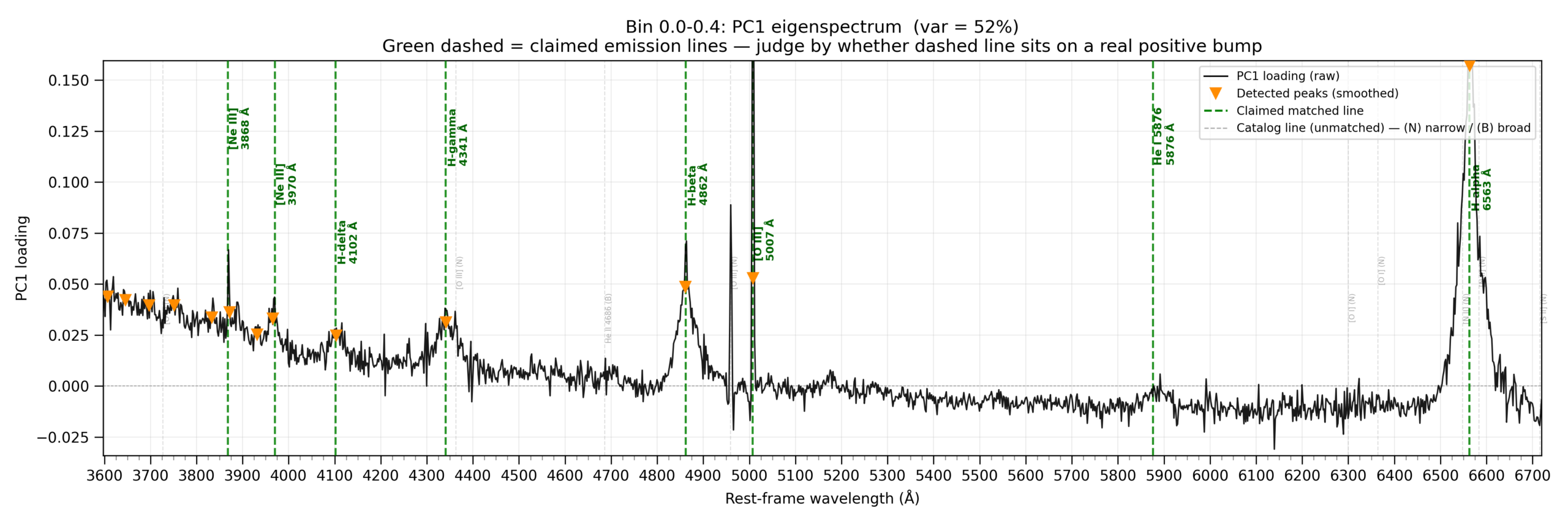
The PC1 eigenspectrum for Bin 1 is shown in Figure 2. The loading is positive at the wavelengths of all looked-at optical emission lines – [Ne III] λ3868, [Ne III] λ3970, Hδ λ4102, Hγ λ4341, Hβ λ4862, [O III] λ5007, and Hα λ6563 – and near-zero or slightly negative between emission lines. [O III] λ5007 carries the largest peak loading (0.271), followed closely by Hα (0.231), confirming both narrow forbidden and broad permitted lines contribute to the emission strength axis.

Hβ exhibits a positive peak (PC1 loading = 0.071 at 4863 Å); Hγ shows a smaller positive peak (loading ~0.038) seen within ~0.5 Å of the catalog wavelength and will be treated as moderate confidence due to a slight possibility of noise.

The narrow [N II] λ6583 and [S II] λ λ6716, 6731 lines are expected to be present but merge with the Hα peak at the 2 Å sampling used here, no conclusions were reached from them.

The continuum regions of the eigenspectrum are essentially flat and close to zero, indicating that an overall slope or trend wasn’t the main difference maker. Rather, PC1 is an “emission-line strength” mode: spectra differ from one another based on how strong their emission lines are relative to the continuum.

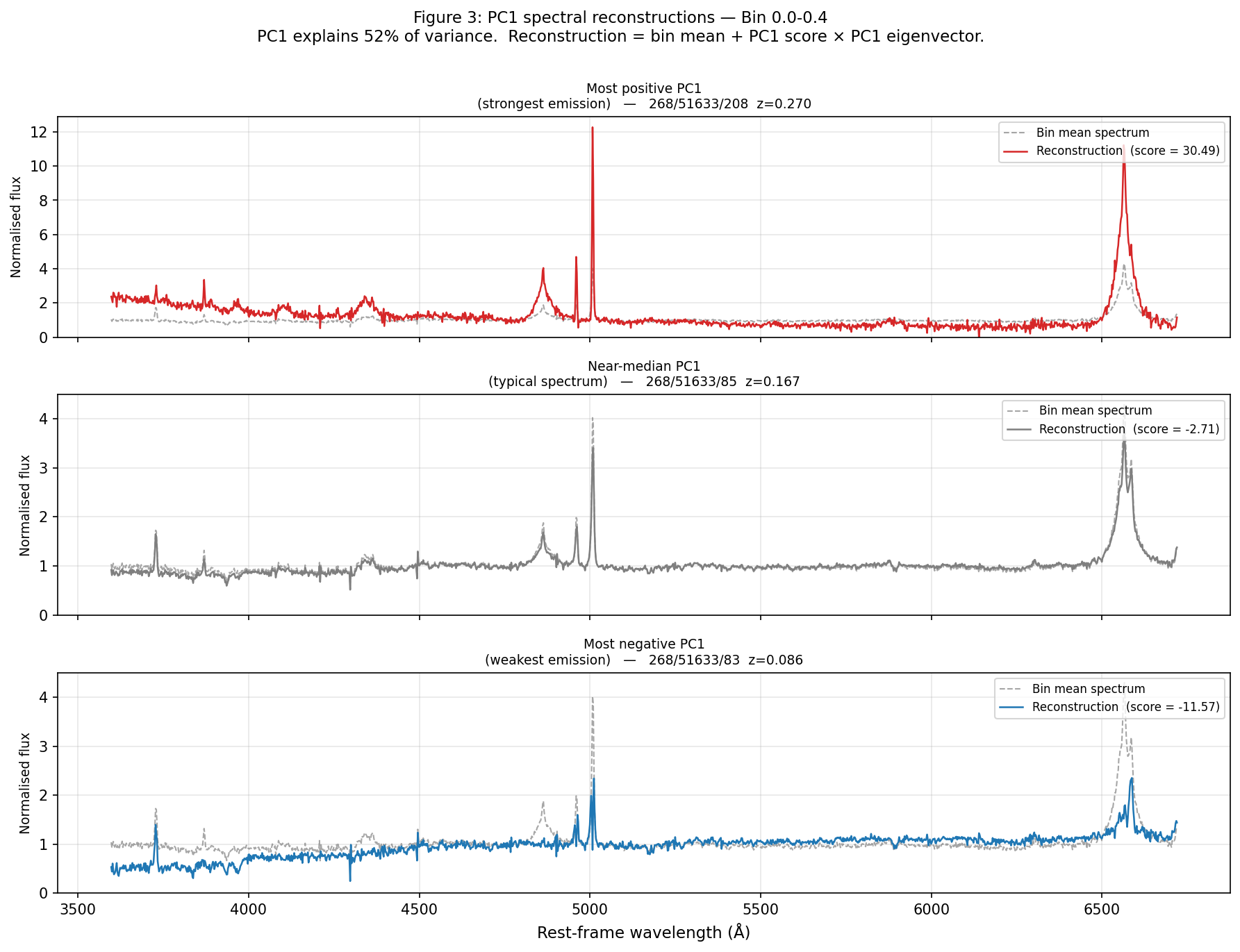
High positive PC1 scores correspond to QSOs with stronger than average emission lines, while negative scores to more emission line weak. Our generated spectral reconstructions (Figure 3) demonstrate this finding: the most negative-score object (s = -11.6) shows a basically featureless continuum, while the highest-score object (s = +30.5) demonstrates obvious Hα, [O III], and Hβ peaks.

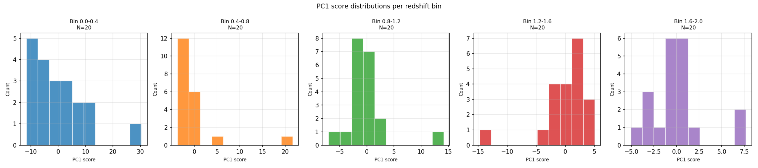
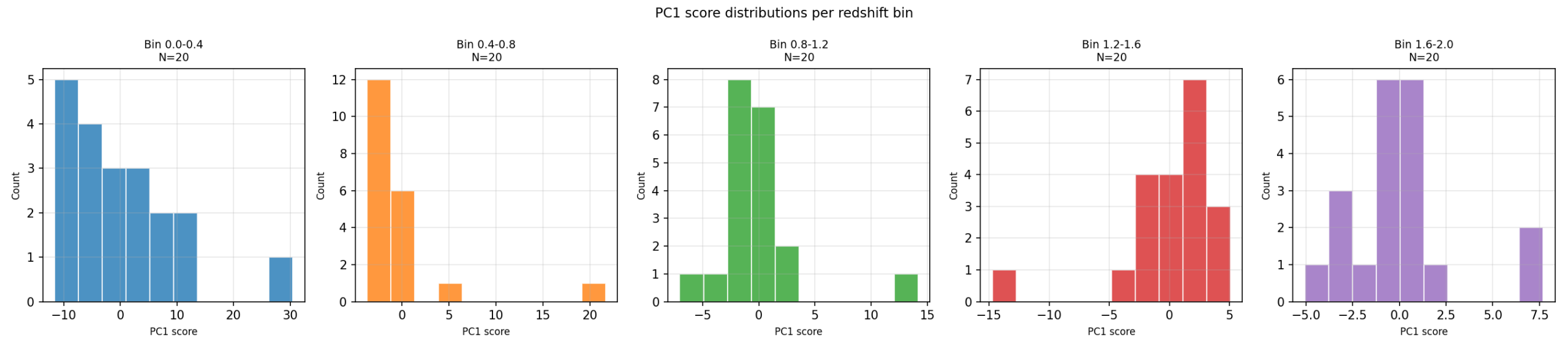
The distribution of PC1 scores in Bin 1 (Figure 4) is the widest, ranging from approximately -12 to +30. This spread is expected, as it reflects the diversity in the low z quasar population in emission line activity. A positive tail extends to high values, corresponding to the subset of objects with especially strong narrow-line emission, which could be QSOs with particularly luminous NLRs. It also includes a negative wing representing objects with little line emission expression. Both populations are expected in our sample sample, since QSO properties span a decent range in emission line equivalent width at any given epoch^4,22.

Secondary components PC2, PC3, and higher explain very significantly less variance (each < 15%). These higher-order components probably encode more subtle variations, such as differences in the ratio of specific lines (e.g., [O III]/Hβ, reflecting ionization state), the power law slope of the AGN continuum, or dust reddening effects. These secondary modes are not analyzed in detail in the present work but could be in future analysis.

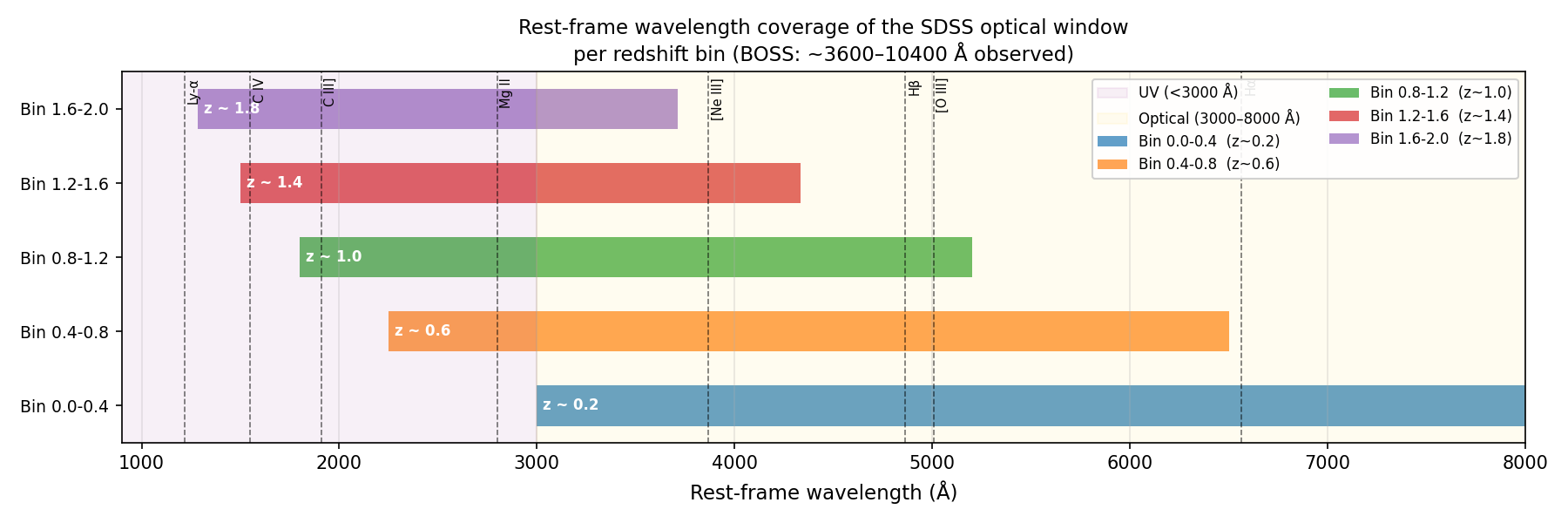
Figure 1 provides context for interpreting the per-bin eigenspectra – the wavelength coverage diagram shows the window accessible to the SDSS spectrograph (observed ∼3800-9200 Å) as a function of the redshift bin. At the center of Bin 1 (z ≈ 0.2), the window spans about ∼3200-7700 Å in the rest frame, covering all optical emission-lines we are looking for (Hβ, [O III], Hα). As redshift increases, this window consistently decreases – at the center of Bin 5 (z ≈ 1.8) the same observed wavelengths correspond to the rest-frame ∼1360-3290 Å, entirely in the UV. This shift explains why the dominant PC1 features change from optical narrow lines in Bin 1 to UV broad lines (C IV, C III]) in Bin 5. It’s a direct consequence of the observable wavelength window, not a change in the “natural” spectrum of the QSOs.

PCA Results for Intermediate Redshift Bins (z ≈ 0.4-1.6)

Moving to higher redshift, Bins 2-4 each contain N = 20 spectra and probe progressively bluer rest-frame wavelengths.

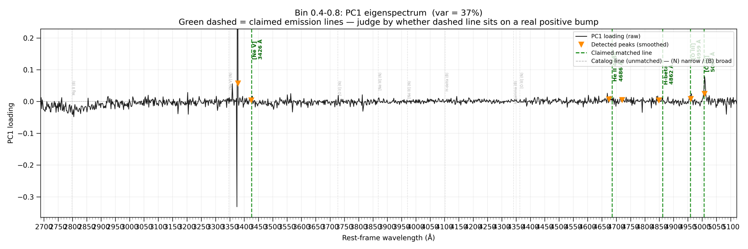
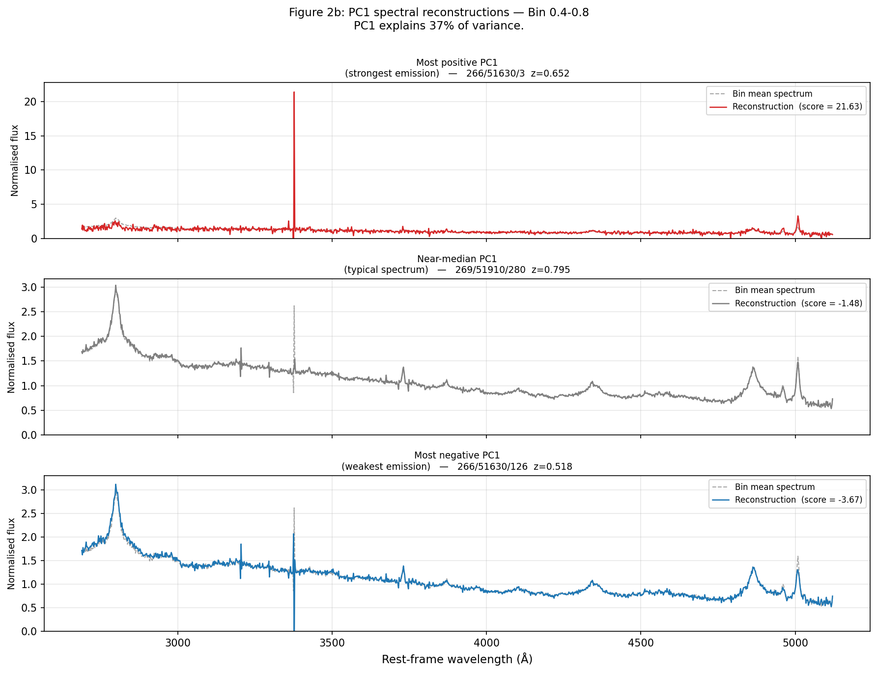
For Bin 2 (z ≈ 0.4-0.8), PC1 accounts for 37% of variance (bootstrap 95% CI: [0.304, 0.693]). The PC1 eigenspectrum (Figure 5) identifies [O III] λ5007 as the dominant confirmed emission feature (loading ~0.075), with [O III] λ4959 (0.025), Hβ (0.010), and [Ne V] λ3426 (0.015) also confirmed on clear eigenspectrum peaks. He II λ4686 is not confirmed: no distinct peak is visible at that wavelength above the local baseline. The [Ne V] λ3426 detection is noteworthy as a high-excitation AGN tracer requiring photons above 97 eV. The narrow spike near 3375 Å in the Bin 2 eigenspectrum coincides with the observed-frame [O I] λ5577 sky line for the highest-scoring object (z = 0.652) and is likely a sky-subtraction residual rather than an astrophysical feature. Spectral reconstructions (Figure 6) show that high-PC1 objects display enhanced [O III] and Hβ emission relative to the bin mean, while low-PC1 objects are more continuum-dominated.

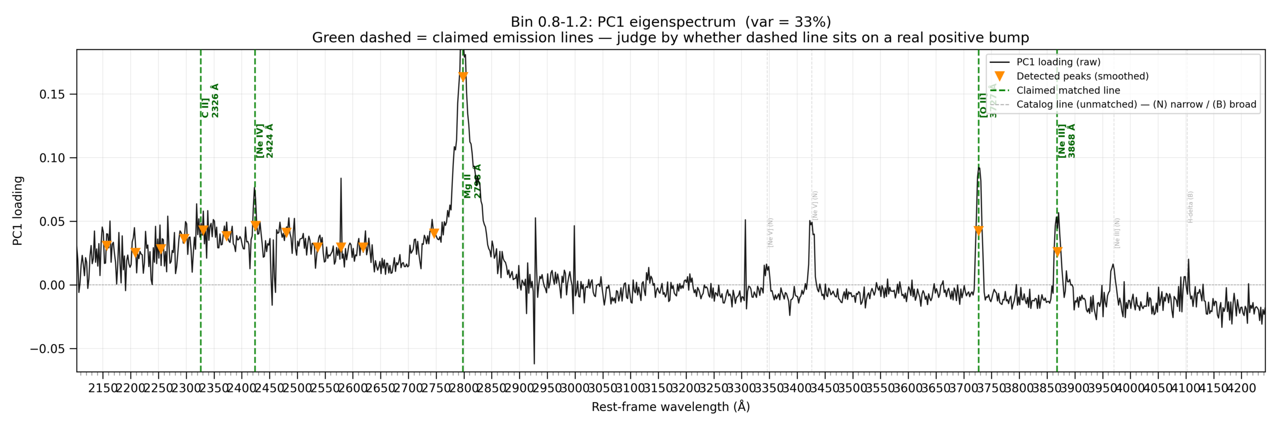
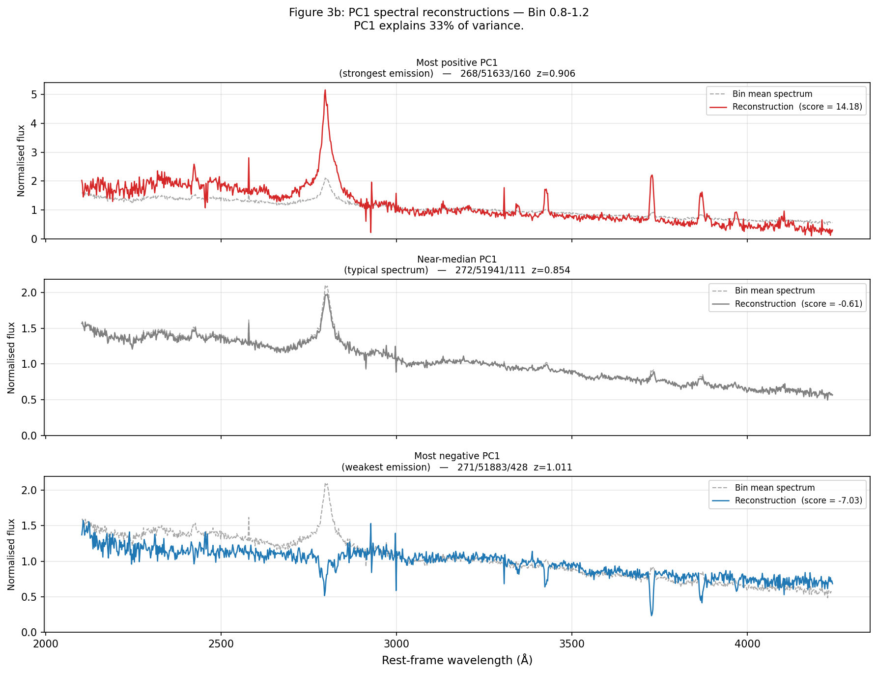
For Bin 3 (z ≈ 0.8-1.2), PC1 accounts for 33% of variance (bootstrap 95% CI: [0.290, 0.661]). The PC1 eigenspectrum (Figure 7) shows fairly certain peaks at [Ne IV] λ2424 (~0.035 above local baseline), Mg II λ2798 (dominant), [Ne V] λ3346 (~0.02), [Ne V] λ3426 (0.05), [O II] λ3727 (0.095), [Ne III] λ3868 (0.06), [Ne III] λ3970 (0.04), and Hδ λ4102 (0.04). Mg II λ2798 is the strongest peak by far, consistent with it being the primary broad permitted line in the near-UV quasar spectrum at this redshift. The two [Ne V] line expressions (λ3346 and λ3426), both high-excitation AGN tracers, are significant as more confirmation of the ionizing AGN continuum. Multiple peaks spanning 2150-2620 Å are consistent with UV Fe II multiplet emission, a complementary pseudo-continuum well known in Type 1 QSOs³⁷. Our spectral reconstructions (Figure 8) confirm that high-PC1 objects show heightened Mg II emission while low-PC1 objects exhibit suppressed near-UV lines.

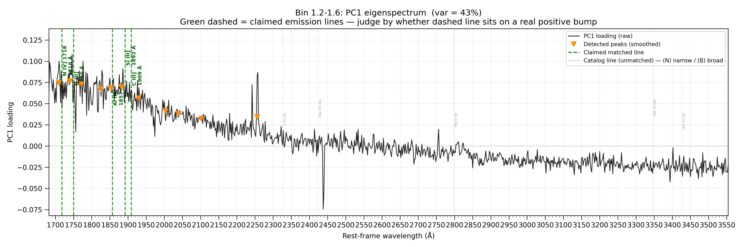
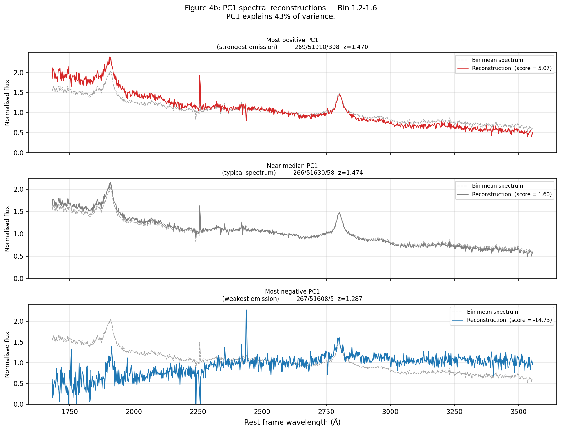
For Bin 4 (z ≈ 1.2-1.6), PC1 accounts for about 43% of variance (bootstrap 95% CI: [0.245, 0.692]). The PC1 eigenspectrum (Figure 9) covers the rest-frame mid- to near-UV (1690-3560 Å), including the ∼1700-2250 Å region, a region with many semi-forbidden and permitted broad lines of the QSO broad-line region: N IV] λ1718, N III] λ1750, Al III λ1857, Si III] λ1892, and C III] λ1909³⁸. The entire 1700-2000 Å region shows a broad, elevated loading pattern (~0.07-0.11) without any obvious peaks above the local baseline – peak heights are comparable in magnitude to the surrounding noise floor (signal-to-baseline ratios of 1.1-1.5), making individual line identifications unreliable. This blending is unfortunately a known property of the mid-UV spectrum, where strong Fe III UV34 emission and intercombination lines fill the 1900 Å area³⁸. Thus, no individual line detections are claimed for Bin 4; instead, we’ll interpret PC1 as capturing overall mid-UV broad-line region emission strength, consistent with the interpretation in all other bins. Our spectral reconstructions (Figure 10) confirm that high-PC1 objects have elevated flux across the entire 1700-2000 Å complex, while low-PC1 objects are comparatively featureless in that range.

Figure 9. PC1 eigenspectrum for Bin 4 (z = 1.2-1.6, N = 20). The 1700-2000 Å region shows a broad elevated loading pattern consistent with the blended mid-UV BLR complex (N III], C III], Si III], Al III). No individual lines are confirmed above the local baseline; PC1 captures overall mid-UV BLR emission strength.

PCA Results at High Redshift (z ≈ 1.6-2.0)

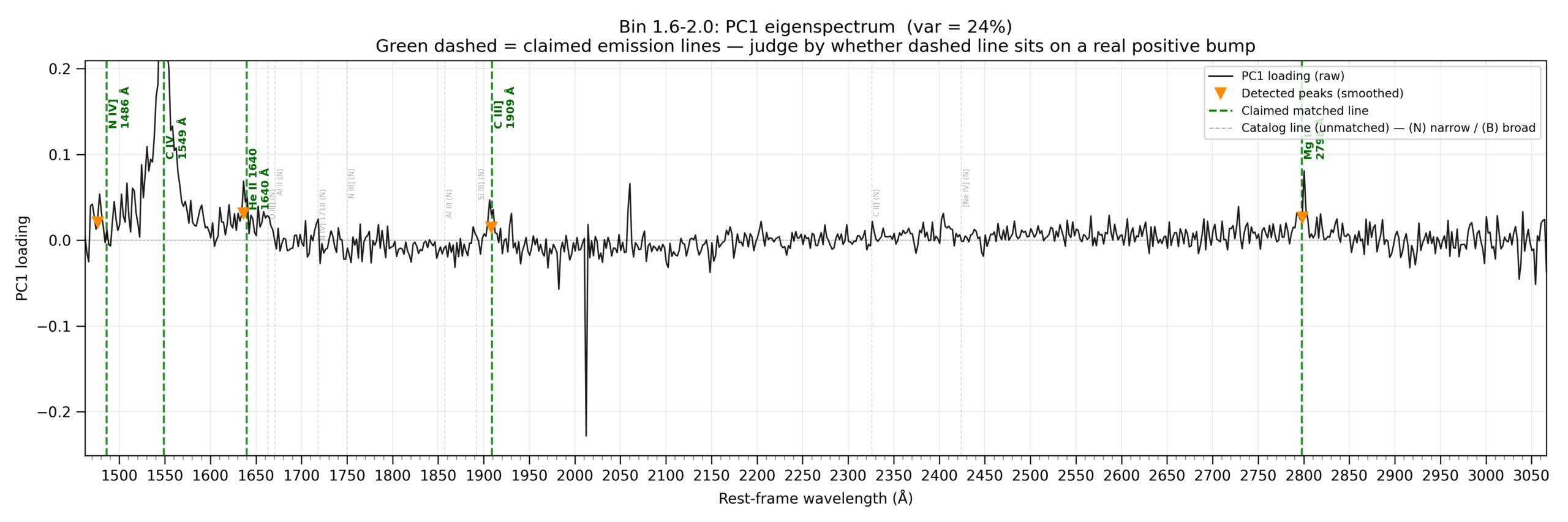
At the highest redshifts (Bin 5, z ≈ 1.6-2.0, N = 20), PC1 accounts for 24% of spectral variance (bootstrap 95% CI: [0.220, 0.453]), which is the lowest fraction across all five bins. UV quasar spectra are known to be more naturally complex than their optical counterparts, with broad line-profile variations and Ly-α forest absorption contributing multiple different variance axes that dilute any single dominant PC. The rest-frame coverage of Bin 5 is 1465-3065 Å, entirely in the UV, where the prominent features are C IV (1549 Å), C III] (1909 Å), and Mg II (2798 Å).

The PC1 eigenspectrum for Bin 5 (Figure 11) explores the rest-frame UV wavelengths (~1465–3065 Å), corresponding to the far- and mid-UV broad-line region. C IV λ1549 shows us the largest positive loading in the bin (raw loading ~0.36-0.40), showing itself as the driver of spectral variance in this bin. He II λ1640 (loading ~0.05 above local baseline), N IV] λ1718 (loading ~0.03 above local baseline), C III] λ1909 (~0.05), and Mg II λ2798 (~0.08) are also confirmed on visible eigenspectrum peaks. He II λ1640, N IV] λ1718, and C III] λ1909 each show a slight blueshift (~1-3 Å) relative to their catalog rest wavelengths, consistent with the known outflow-driven blueshifts of UV emission lines in Type 1 QSOs³⁸. As in all other bins, the inter-line continuum loading is near zero, confirming that PC1 encodes relative UV emission-line strength rather than overall continuum trends.

There exists a large contrast between the first and last bin. In the first, with z ≈ 0.0-0.4, the SDSS optical window covers rest-frame ~3600–6730 Å, yielding eigenspectra mostly covered by [O III] λ5007 and Hα. At z ≈ 1.6-2.0, the same observed window corresponds to rest-frame 1465-3065 Å, entirely in the UV, and the dominant contributor is C IV λ1549 – the strongest broad permitted line in the given spectrum. The two PC1 eigenspectra thus examine physically different line forming regions and can’t be compared feature by feature.

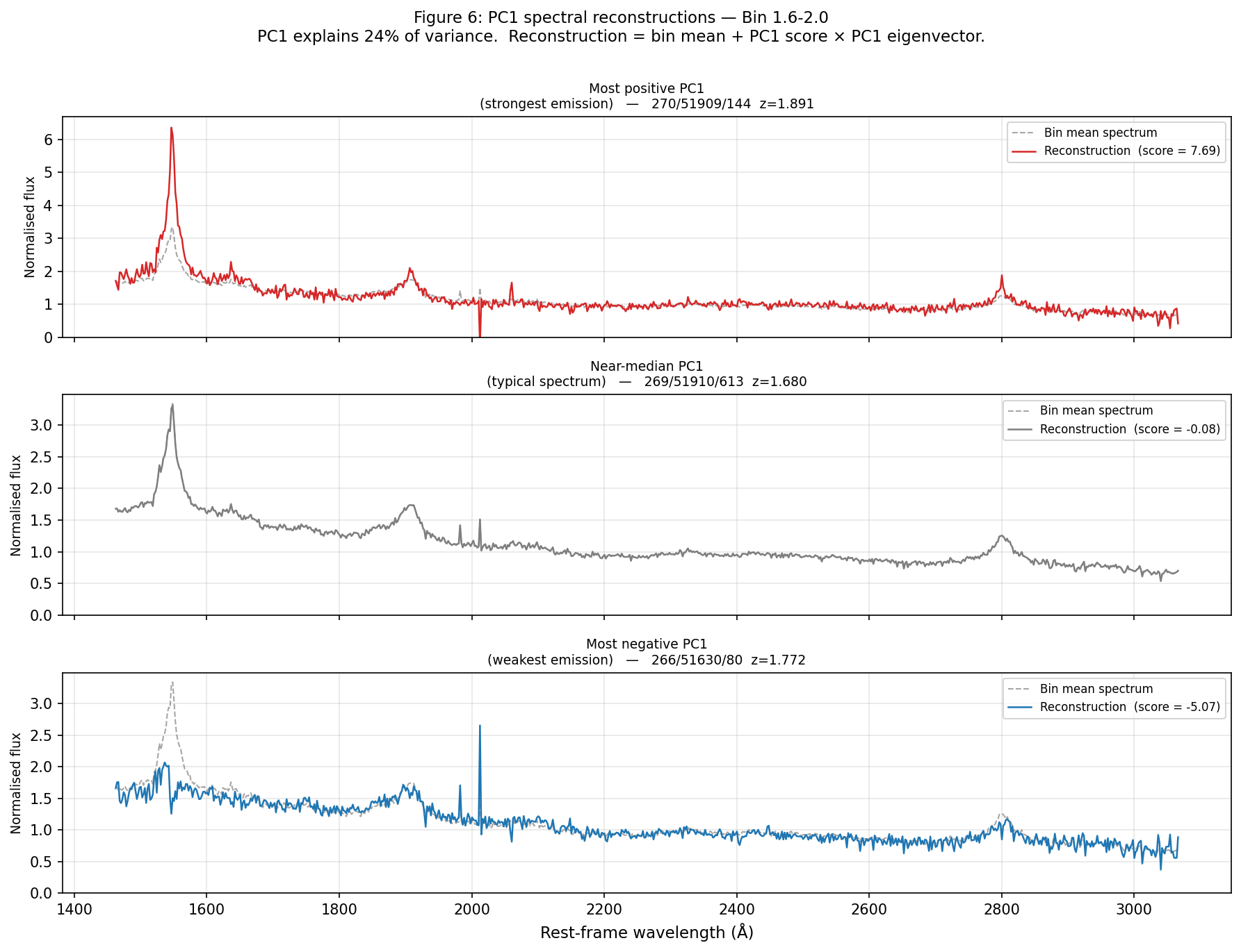
Example reconstructions for Bin 5 can be seen in Figure 12, below. The spectra with the highest PC1 score (s = +7.7) shows heightened UV broad-line emission with higher C IV and C III] features relative to the bin mean. The object with the most negative PC1 score (s = -5.1) shows suppressed UV emission as expected, consistent with a more continuum-dominated QSO.

The PC1 score histogram for Bin 5 (Figure 13) is shaped differently than the Bin 1 histogram. The distribution is narrower and concentrated near zero, with scores spanning roughly -5 to +8. Notably, there’s no extended negative tail corresponding to weak-line QSOs. This makes sense, as it is consistent with the expectation that AGN emission-line activity is consistently present at cosmic noon, when accretion rates and star formation were globally elevated^33,11. However, we must note that SDSS QSO classification inherently requires detectable emission features, so any genuinely passive absorption-line objects at z ≈ 1.6-2.0 simply would not appear in this sample.

The comparison is best read as highlighting the difference between two quasar-selected samples at different epochs, not as a statement about the broader galaxy population.

To quantify the difference in PC1 score distributions between Bin 1 and Bin 5, a two-sample Kolmogorov-Smirnov experiment was run to the raw PC1 scores. The test yielded d = 0.40, p = 0.081 (n_1 = n_5 = 20). This result doesn’t reach significance at the alpha = 0.05 level but gets close, suggesting a slight tendency toward a difference in distribution. With equal samples of n = 20, the KS test has more power than the earlier n= 15 and n = 5 configuration (p = 0.55), where even a true d = 0.40 would rarely be detected. When scores are normalized to zero mean and unit variance before the test (removing the confound of different score scales between bins), d = 0.15, p = 0.98, showing that the raw score offset is driven by differences in overall scale rather than in the shape of the distribution. Expanding the per-bin sample to n ≥ 30 could yield us more conclusions about whether the distributional shapes actually make a difference.

Comparative Discussion

Across all five bins, PC1 for the most part encodes variation in emission-line strength relative to the continuum – a consistent result regardless of redshift or rest-frame wavelength range. This result is also consistent with prior PCA studies of QSO spectra, in which emission-line strength is a leading axis of variation; Francis et al. (1992)²² identified emission-line core strength as a leading principal component. Ma et al. (2019)²⁵ identify the leading QSO principal component with the well-known Eigenvector 1 anticorrelation between [O III] and Fe II. Yip et al. (2004)²³ also showed that SDSS quasar eigenspectra reflect redshift and luminosity dependent physical conditions, which helped motivate the per-bin approach used here.

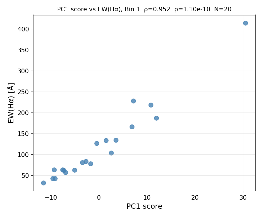
That said, the emission-strength interpretation is confirmed measureably only for Bin 1 (Spearman ρ = 0.952 with EW(Hα), N = 20).

In the UV bins (Bins 3-5), PC1 increasingly encodes a mixture of UV emission-line strength and UV continuum slope, which are effects partially covariant in Type 1 QSO spectra^23,39. Establishing the emission strength interpretation for UV bins would require per-bin Spearman correlations against bin-appropriate proxies (e.g., EW(C IV) for Bin 5, EW(Mg II) for Bins 3-4), which are put into future work.

The difference lies in the distributional properties of the PC1 scores. At low z (Bin 1), the score distribution spans approximately -12 to +30, demonstrating significant range in AGN emission line expression. At high z (Bin 5), the scores are concentrated between -5 and +8 without an extended tail, which the other bins had.

These distributional differences are consistent with the known evolution in cosmic AGN activity. QSO luminosity functions are known to peak at z ≈ 2 and decline toward the present³³, so higher redshift QSO samples tend to be more uniformly active. The caveat about QSO selection (described above) must be thought of when interpreting this comparison as evidence for cosmological evolution per se.

The shift in dominant emission-line contributors of [O III] λ5007 and Hα at low z (Bin 1) to C IV λ1549 at high z (Bin 5) is likely primarily due to the difference in rest frame wavelength coverage. At z ≈ 0.0-0.4, the SDSS window covers rest-frame optical lines, while at at z ≈ 1.6-2.0, the window covers rest-frame UV broad-line emission only. The [O III] and Hβ lines in Bin 1 are shifted to observed wavelengths ≳12,600 Å at z ≈ 1.6 and are completely outside the SDSS spectral range for Bins 4-5 (see Cross-bin comparability in Limitations). When the differences between bins are really due to evolution, it’s because galaxies in the older bins had more radiation and less metal-rich gas. This leads to high energy UV lines like C IV, which matches what they actually saw as the strongest signal in their most distant bin^11,31,12,14.

The interpretation of PC1 as an “emission-line strength” axis can be strongly suggested measureably by matching the PC1 scores with directly measured Hα equivalents for Bin 1. Hα equivalent widths were derived from each of the de-redshifted spectra by exercising the continuum-normalized flux within a +/- 40 Å window centered on Hα (6564.6 Å), and using sidebands at +/- 80-120 Å to estimate.

The Spearman rank correlation between PC1 score and EW(Hα) is ρ = 0.952, p = 1.1 x 10^-10 (N = 20; Figure 14). This correlation shows that objects with higher PC1 scores have stronger Hα emission, directly establishing PC1 as an emission-line strength axis rather than an artifact of the PCA preprocessing. The relationship is consistent across the full range of scores in Bin 1, from the most continuum trend heavy to the most strongly emission-line-expression-heavy QSOs in the sample.

Limitations

Several limitations apply, such as:

Sample size

Each bin contains n = 20 spectra after the quality cut, attained by querying an attempted 500 QSO per bin and accepting the first 20, so long as they meet the quality requirement.

While our n = 20 represents an improvement over previous analyses with n = 5-15 per bin, it’s still below the n ≥ 50-100 typically recommended for “robust” PCA eigenvector estimation. At n = 20, even one radically contrasting QSO can still shift eigenvectors, though the risk is significantly smaller when compared to N = 5. Bootstrap resampling (500 resamples) was performed for all bins, a standard practice, and the resulting 95% confidence intervals on the PC1 variance fraction are [0.475, 0.715] for Bin 1, [0.304, 0.693] for Bin 2, [0.290, 0.661] for Bin 3, [0.245, 0.692] for Bin 4, and [0.220, 0.453] for Bin 5, with each of the original ranges being in those intervals. The “older” intervals, particularly for Bins 2-4, show sampling uncertainty at n = 20.

The KS test between Bin 1 and Bin 5 (d = 0.40, p = 0.081, n_1 = n_5 = 20) approaches but quite get to the alpha = 0.05 significance threshold, so a potential sample of N ≥ 30 per bin could provide the perspective needed to resolve this issue.

Cross-bin comparability

Bins 4 and 5 see rest-frame UV wavelengths with no overlap with the optical coverage of Bins 1-2. No common rest-frame wavelength window exists across all five bins. A shared-basis PCA was performed for Bins 1-3 over their common wavelength window (3810-4180 Å), showing and confirming a dominant PC1 in Bins 1 and 3 but yielding low PC1 variance (33%) for Bin 2 in this narrow window. The cross-bin comparison in this study is thus naturally qualitative for Bins 1-3 and unfortunately essentially impossible for Bins 4-5 relative to low-z bins, since these higher z bins explore a completely different wavelength and thus completely different physical meanings.

This is a limitation that can’t be fixed without near-infrared spectroscopy to access rest-frame optical features at z > 0.8.

Preprocessing sensitivity

The normalization method, mean subtraction method, and treatment of sky and bad pixels can all influence the PCA results. For instance, normalization on the median flux (without masking of emission lines) is not the same as normalization in a line-empty continuum region. These different normalization methods can influence the amplitudes of the emission lines in the normalized data and thus can influence the character of PC1. The near zero loadings in the PC1 eigenspectrum in the continuum regions could be an effect of the mean subtraction rather than a physically meaningful line-only mode. Tests exploring the effects of different normalization methods (with and without masking of emission lines, median normalization vs. normalization in the 4400-4600 Å line-empty region).

Selection effects

Our high-z sample contains only spectroscopic QSOs that are selected by the presence of emission lines. For this reason, claims about the manifestation of the “emergence of passive galaxies” in the differences between the distributions in the PC1 parameter for low-z versus high-z must be tempered. We are comparing the distributions for two samples of emission line selected QSOs at different redshifts, and not population complete samples of galaxies. A more rigorous comparison would involve either selecting analogously QSOs in both the low-z and high-z samples and quantifying the incompleteness in the difference between these samples, or employing a magnitude or mass.

Physical parameter correlations for higher-redshift bins

Our interpretation of PC1 as an emission-line strength axis has been confirmed for Bin 1 by direct correlation with EW(Hα) (Spearman ρ = 0.952, p = 1.1 x 10^-10, N = 20). However, as discussed in the cross bin comparability, verification has not been extended to higher-redshift bins, specifically, where Hα falls outside the SDSS optical window and alternative lines such as EW([O III] λ5007), EW(Mg II λ2798), or AGN bolometric luminosity would be required.

Conclusion

We used PCA on 100 QSO spectra from SDSS DR16 in five redshift bins (z = 0 to z = 2) with N = 20 spectra in each bin. To select the spectra in each bin up to 500 candidates were queried and the first 20 accepted with a median S/N > 5. PC1 explains 52%, 37%, 33%, 43% and 24% of the total spectral variance in Bins 1-5, respectively. The eigenspectrum of PC1 in each bin exhibits emission lines as peaks and has low amplitude between lines. This is encouraging for an emission line strength as a primary source of spectral difference. We can confirm this in Bin 1 by finding a Spearman correlation of PC1 scores with observed Hα equivalent width of ρ = 0.952 (p = 1.1 x 10^-10 for N = 20). In the highest redshifts (Bin 5: UV at rest frame 1465-3065 Å), C IV λ1549 has a significant contribution to the eigenspectrum (loading ≈ 0.36-0.40) which is again indicative of emission strength being the primary source of difference in the UV.

There is also a qualitatively plausible evolution in PC1 distributions across epochs. At low redshift (z ≈ 0.0-0.4) there is a large range of objects from weak-line to strong-line QSOs. At high redshift (z ≈ 1.6-2.0) there is a smaller distribution skewed to the right with little weak-line tail. This is plausible for the more homogeneously emitting QSOs during cosmic noon. A KS test was performed on the raw PC1 values and gives d = 0.40, p = 0.081 (n_1 = n_5 = 20). This is only marginally significant at alpha = 0.05. This could be improved with N ≥ 30 per bin. The main emission lines contributing to the distribution change from Hα and [O III] in Bin 1 (rest-frame optical at low z) to UV broad emission lines C III] λ1909 and C IV λ1549 in Bin 5 (rest-frame UV at high z). This is most likely due to changing rest-frame observables and not a change in the physics of the emission lines themselves. For systems with clear astrophysical evolution, one would expect decreased gas metallicity and stronger ionizing radiation at z ≈ 2 to enhance high- ionization UV emission^11,31,12,14.

Some major restrictions in this study include the relatively small sample size per bin (n = 20) which, though constant and an improvement from previous studies, falls below the minimum sample size of n ≥ 50-100 required for stable eigenvectors. Another restriction is the lack of a common-basis PCA between all five bins because they do not cover the same rest-frame wavelengths. The PCA is also sensitive to the method of normalization used. Finally, the sample of high-z objects is selected on QSOs which also introduces selection effects. All of these issues should be considered in future studies prior to claiming strong evidence for evolution.

Future directions include:

(1) Expanding the analysis to hundreds of spectra per bin, using the full SDSS DR16 QSO catalog²⁸;

(2) Extending the shared basis PCA beyond the 3810-4180 Å window demonstrated here for Bins 1-3, by acquiring rest-frame optical coverage at z > 0.8 via near-infrared spectroscopy (though this may add a calibration layer of complexity);

(3) Use correlations between PC1 for different high-redshift bins and proxies for the emission lines, such as EW([O III] λ5007), EW(Mg II λ2798), or bolometric luminosity of an AGN, to test if the relation found for Bin 1 also holds in the UV covered by Bins 3-5;

(4) Use higher PCs (PC2, PC3) to explore other sources of spectral differences: ionization, line width, continuum slope, etc;

(5) Move into the near-infrared with JWST/NIRSpec to observe rest-frame optical emission lines (Hα, [O III]) at z > 1, allowing direct cross-bin comparisons in a shared rest-frame wavelength range.

PCA therefore provides a minimal-assumptions, data-oriented approach to understanding the evolution of spectral diversity in galaxies with redshift. The most important spectral component in each redshift bin is emission lines. The shift in the PC1 distribution between z ≈ 2 and z ≈ 0, despite the need for careful handling of selection effects, also agrees generally with the evolution of AGN and galaxy populations with redshift. The dominance of emission lines in the same spectral component across five redshift bins covering approximately 10 billion years of lookback time appears to indicate that the physics behind active nuclei, although evolving in strength, may remain fundamentally similar throughout the cosmic history.

Supplementary Information

References

1. Kewley, L. J., & Dopita, M. A. (2002). Using strong lines to estimate abundances in extragalactic H II regions and starburst galaxies. Astrophys. J. Suppl., 142(1), 35-52. DOI: 10.1086/341326 [↩]
2. Tremonti, C. A., et al. (2004). The origin of the mass-metallicity relation: Insights from 53,000 star-forming galaxies in the SDSS. Astrophys. J., 613(2), 898-913. DOI: 10.1086/423264 [↩] [↩] [↩] [↩] [↩]
3. Kewley, L. J., & Ellison, S. L. (2008). Metallicity calibrations and systematic effects. Astrophys. J., 681(2), 1183-1204. DOI: 10.1086/587500 [↩] [↩] [↩] [↩] [↩] [↩] [↩]
4. Netzer, H. (2015). Revisiting the unified model of active galactic nuclei. Annu. Rev. Astron. Astrophys., 53, 365-408. DOI: 10.1146/annurev-astro-082214-122302 [↩] [↩] [↩] [↩] [↩] [↩] [↩] [↩]
5. Veilleux, S., & Osterbrock, D. E. (1987). Spectral classification of emission-line galaxies. Astrophys. J. Suppl., 63, 295-310. DOI: 10.1086/191166 [↩] [↩] [↩]
6. Kennicutt, R. C. (1998). Star formation in galaxies along the Hubble sequence. Annu. Rev. Astron. Astrophys., 36, 189-232. DOI: 10.1146/annurev.astro.36.1.189 [↩] [↩]
7. Thomas, D., et al. (2005). The epochs of early-type galaxy formation as a function of environment. Astrophys. J., 621(2), 673-694. DOI: 10.1086/427281 [↩] [↩] [↩]
8. Baldwin, J. A., Phillips, M. M., & Terlevich, R. (1981). Classification parameters for the emission-line spectra of extragalactic objects. Publ. Astron. Soc. Pacific, 93(549), 5-19. DOI: 10.1086/130766 [↩] [↩] [↩]
9. Maiolino, R., Nagao, T., Grazian, A., et al. (2008). AMAZE. I. The evolution of the mass-metallicity relation at z > 3. Astron. Astrophys., 488(2), 463-479. DOI: 10.1051/0004-6361:200809678 [↩] [↩]
10. Zahid, H. J., Kashino, D., Silverman, J. D., et al. (2014). The FMOS-COSMOS survey of star-forming galaxies at z ~ 1.6. II. The mass-metallicity relation and the dependence on star formation rate and dust extinction. Astrophys. J., 792(2), 75. DOI: 10.1088/0004-637X/792/2/75 [↩] [↩]
11. Steidel, C. C., et al. (2014). Strong nebular line ratios in the spectra of z~2-3 star-forming galaxies: First results from KBSS-MOSFIRE. Astrophys. J., 795(2), 165. DOI: 10.1088/0004-637X/795/2/165 [↩] [↩] [↩] [↩] [↩] [↩] [↩] [↩]
12. Shapley, A. E., et al. (2015). Rest-optical spectroscopy of z~2 star-forming galaxies: evidence for ubiquitous high ionization states and evolving physical conditions. Astrophys. J., 801(1), 88. DOI: 10.1088/0004-637X/801/1/88 [↩] [↩] [↩] [↩] [↩]
13. Sanders, R. L., Shapley, A. E., Kriek, M., et al. (2016). The MOSDEF survey: excitation properties at z~2.3 and implications for the BPT diagram. Astrophys. J., 816(1), 23. DOI: 10.3847/0004-637X/816/1/23 [↩] [↩]
14. Strom, A. L., Steidel, C. C., Rudie, G. C., et al. (2017). Nebular emission-line ratios in z~2 KBSS galaxies. Astrophys. J., 836(2), 164. DOI: 10.3847/1538-4357/836/2/164 [↩] [↩] [↩] [↩]
15. Garg, P., Narayanan, D., Byler, N., et al. (2022). The BPT diagram in cosmological galaxy formation simulations: understanding the physics driving offsets at high redshift. Astrophys. J., 926(1), 80. DOI: https://doi.org/10.3847/1538-4357/ac43b8 [↩] [↩] [↩]
16. Sanders, R. L., Shapley, A. E., Jones, T., et al. (2024). Direct Te-based metallicities of z ~ 2-9 star-forming galaxies with JWST/NIRSpec. Astrophys. J., 962(1), 24. DOI: 10.3847/1538-4357/ad04b5 [↩] [↩]
17. Hirschmann, M., Charlot, S., Somerville, R. S., et al. (2023). Simulating the diversity of galaxy emission-line properties and biases in z = 0 metallicity calibrations at high redshift. Mon. Not. R. Astron. Soc., 526(3), 3630-3656. DOI: 10.1093/mnras/stad2955 [↩] [↩]
18. Laseter, I. H., Maseda, M. V., Curti, M., et al. (2024). JADES: Detecting [O III]λ4363 emitters and testing strong line calibrations in the high-z Universe with ultra-deep JWST/NIRSpec spectroscopy up to z ~ 9.5. Astron. Astrophys., 681, A70. DOI: 10.1051/0004-6361/202347133 [↩] [↩] [↩]
19. Curti, M., Maiolino, R., Curtis-Lake, E., et al. (2023). The chemical enrichment in the early Universe as probed by JWST via direct metallicity measurements at z ≈ 8. Mon. Not. R. Astron. Soc., 518(1), 425-438. DOI: 10.1093/mnras/stac2737 [↩] [↩]
20. Yip, C. W., et al. (2004). Distributions of galaxy spectral types in the Sloan Digital Sky Survey. Astron. J., 128(2), 585-609. DOI: 10.1086/422429 [↩] [↩] [↩]
21. Wild, V., Kauffmann, G., Heckman, T., et al. (2007). Bursty stellar populations and obscured AGN in galaxy bulges. Mon. Not. R. Astron. Soc., 381(2), 543-572. DOI: 10.1111/j.1365-2966.2007.12256.x [↩]
22. Francis, P. J., Hewett, P. C., Foltz, C. B., Chaffee, F. H. (1992). An objective classification scheme for QSO spectra. Astrophys. J., 398, 476–490. DOI: 10.1086/171870 [↩] [↩] [↩] [↩]
23. Yip, C. W., Connolly, A. J., Berk, D. E., et al. (2004). Spectral classification of quasars in the Sloan Digital Sky Survey: eigenspectra, redshift, and luminosity effects. Astron. J., 128(6), 2603-2629. DOI: 10.1086/425626 [↩] [↩] [↩]
24. Pâris, I., Petitjean, P., Rollinde, E., et al. (2011). A principal component analysis of quasar UV spectra at z ~ 3. Astron. Astrophys., 530, A50. DOI: https://doi.org/10.1051/0004-6361/201016233 [↩]
25. Ma, B., Shang, Z., Brotherton, M. S. (2019). Spectral principal component analysis of the Hβ region of low-redshift SDSS quasars. Res. Astron. Astrophys., 19(12), 169. DOI: https://doi.org/10.1088/1674-4527/19/12/169. [↩] [↩]
26. Suzuki, N. (2006). Quasar spectrum classification with principal component analysis: emission lines in the Lya forest. Astrophys. J. Suppl., 163(1), 110-121. DOI: 10.1086/499272 [↩]
27. Ahumada, R., Prieto, C. A., Almeida, A., et al. (2020). The 16th Data Release of the Sloan Digital Sky Surveys: First Release from the APOGEE-2 Southern Survey and Full Release of eBOSS Spectra. Astrophys. J. Suppl., 249(1), 3. DOI: 10.3847/1538-4365/ab929e [↩] [↩] [↩]
28. Lyke, B. W., Higley, A. N., McLane, J. N., et al. (2020). The Sloan Digital Sky Survey Quasar Catalog: Sixteenth Data Release. Astrophys. J. Suppl., 250(1), 8. DOI: 10.3847/1538-4365/aba623 [↩] [↩] [↩]
29. Leitherer, C., Schaerer, D., Goldader, J. D., et al. (1999). Starburst99: synthesis models for galaxies with active star formation. Astrophys. J. Suppl., 123(1), 3-40. DOI: 10.1086/313233 [↩]
30. Pettini, M., & Pagel, B. E. J. (2004). [O III]/[N II] as an abundance indicator at high redshift. Mon. Not. R. Astron. Soc., 348(1), L59–L63. DOI: 10.1111/j.1365-2966.2004.07198.x [↩]
31. Kewley, L. J., et al. (2013). Theoretical evolution of optical strong lines across cosmic time. Astrophys. J., 774(2), 100. DOI: 10.1088/0004-637X/774/2/100 [↩] [↩] [↩] [↩] [↩] [↩]
32. Brinchmann, J., et al. (2004). The physical properties of star-forming galaxies in the low-redshift universe. Mon. Not. R. Astron. Soc., 351(4), 1151-1179. DOI: 10.1111/j.1365-2966.2004.07881.x [↩]
33. Madau, P., & Dickinson, M. (2014). Cosmic star-formation history. Annu. Rev. Astron. Astrophys., 52, 415-486. DOI: 10.1146/annurev-astro-081811-125615 [↩] [↩] [↩] [↩] [↩] [↩] [↩]
34. Erb, D. K., et al. (2006). The mass-metallicity relation at z ~ 2. Astrophys. J., 644(2), 813-828. DOI: 10.1086/503623 [↩]
35. Kewley, L. J., Dopita, M. A., Leitherer, C., et al. (2013). The Cosmic BPT Diagram: Confronting Theory with Observations. Astrophys. J. Lett., 774(1), L10. DOI: 10.1088/2041-8205/774/1/L10 [↩] [↩]
36. Pedregosa, F., Varoquaux, G., Gramfort, A., et al. (2011). Scikit-learn: Machine learning in Python. J. Mach. Learn. Res., 12, 2825-2830. [↩]
37. Vestergaard, M., & Wilkes, B. J. (2001). An empirical ultraviolet template for iron emission in quasars as derived from I Zwicky 1. Astrophys. J. Suppl., 134(1), 1-37. DOI: 10.1086/320357 [↩]
38. Vanden Berk, D. E., et al. (2001). Composite quasar spectra from the Sloan Digital Sky Survey. Astron. J., 122(2), 549-564. DOI: 10.1086/321167 [↩] [↩] [↩]
39. Boroson, T. A., & Green, R. F. (1992). The emission-line properties of low-redshift quasi-stellar objects. Astrophys. J. Suppl., 80, 109-135. DOI: 10.1086/191661 [↩]