A Statistical Physics Approach to Market Dynamics: Regime Shifts in Digital vs. Local Vendor Choice

July 12, 2026

Abstract

Digital commerce platforms compete with local vendors under frictions of time, price, and visibility. We test whether an interpretable choice model with reinforcement and social influence can yield substantial changes in aggregate market share as control parameters vary. We simulate repeated customer choice among vendors using a utility function that combines vendor attributes (price, delivery or travel time, rating), reinforcement from past interactions (optionally decayed), and a prior-popularity social term. Choices follow a Boltzmann rule with temperature (T) controlling decision noise. An information parameter (γ) controls discovery of local options; (γ=0) keeps locals invisible and yields zero local purchases by construction. We measure late-time local share, market concentration (HHI), and diversity (entropy). In a baseline setting (T=0.5), (γ=0.3), (φ=0.2), the market is concentrated and local share is low ( $\approx$ 0.17). Enabling an Open Network for Digital Commerce (ONDC)-style protocol and increasing the protocol distance weight (w) increases local competitiveness at the same (T) and (γ). Late local share rises from ( $\approx$ 0.17) (w=0) to ( $\approx$ 0.55) (w=1), and market concentration falls correspondingly (HHI from ( $\approx$ 0.64) to ( $\approx$ 0.30); entropy from ( $\approx$ 0.79) to ( $\approx$ 1.44). A (γ x w) interaction slice shows that (γ) gates local participation (local share ( $\approx$ 0) for (γ=0) at all (w), while (w) modulates outcomes once locals are discoverable (γ>0), including at (γ=1). These results connect utility-based choice to macroscopic outcomes and isolate how information frictions and distance-weighted protocols affect platform–local competition.

Keywords: agent-based modeling; consumer choice; information frictions; market concentration; regime shifts

Introduction

Background and context

Digital commerce has fundamentally changed the way consumers shop and the way markets are organized. Large online platforms have grown rapidly by exploiting network effects—the tendency of a service to become more valuable as more people use it.¹ This creates a self-reinforcing cycle in which dominant sellers attract more buyers, and more buyers attract more sellers. Research on two-sided market theory explains how these dynamics can lock entire markets into configurations where one or a few players capture a disproportionate share of all transactions, making it structurally difficult for newer or smaller sellers to compete.² A related phenomenon is technological lock-in: once consumers settle on a particular platform or seller, switching costs and habit formation keep them there even when alternatives might be equally good.³

One group that is especially disadvantaged by these dynamics is local vendors—small, geographically-rooted sellers who may offer competitive prices, faster delivery for nearby customers, and direct community relationships, but who lack the algorithmic visibility and marketing budgets of large digital platforms. While digital platforms have created substantial consumer welfare through increased product variety and lower search costs,⁴ this welfare gain is unevenly distributed: in many cases, customers may not know that a local vendor exists at all, even when that vendor would be a rational choice. This type of structural invisibility can produce what economists call information cascades: consumers continue buying from well-known sellers not because those sellers are objectively better, but simply because they have never been exposed to the alternatives.⁵^,⁶ Direct empirical evidence for this mechanism includes experimental studies showing that social influence amplifies inequality among otherwise similar options,⁷ and analyses of online retail in which information frictions and search costs shape both pricing and the share of demand captured by less prominent sellers.⁸

This paper approaches these dynamics through a physics-inspired lens. Researchers in the fields of econophysics and sociophysics have shown that the tools of statistical physics—originally developed to describe how atoms and molecules behave collectively—can also be applied to describe how large groups of people make decisions in markets and social systems.⁹^,¹⁰^,¹¹ A particularly powerful concept borrowed from physics is the phase transition: the idea that a system can shift abruptly from one qualitatively different state to another when a key control parameter crosses a threshold, much as water transitions sharply from liquid to ice at a specific temperature.¹²^,¹³ Markets can behave similarly. A market that begins in a diverse, balanced state can, under conditions of increasing social influence or growing information asymmetry, shift toward a winner-take-most configuration.¹⁴ The present model does not exhibit a strict phase transition: the changes we observe in aggregate outcomes are smooth rather than abrupt. The analogy remains valuable, however, because it draws attention to a small number of interpretable control parameters—noise, information access, and social influence—that govern which regime the system occupies.

Problem statement and rationale

We ask: How do randomness in individual choice and information frictions about local vendors shape the long-run market share of local commerce? Two mechanisms are of particular interest. First, we model a temperature-like parameter T that controls how strongly customers follow utility differences versus exploring at random—a formalization grounded in the statistical mechanics of decision-making.¹⁵^,¹⁶ Second, we model an information-access rate γ that controls how quickly customers discover local vendors who were initially invisible to them. We also consider a social-influence term that biases customers toward vendors that were popular in the previous round, drawing on a long tradition of models in which social interactions generate multiple possible market equilibria depending on the strength of conformity, and in which herd behavior contributes substantially to aggregate market fluctuations.¹⁷^,¹⁸^,¹⁹

Understanding these mechanisms matters because information frictions are not simply a byproduct of market competition—they are often a structural feature that policy interventions can change. If altering information access can move a market from a concentrated, digital-dominant regime to a more balanced one, then such interventions can be studied and evaluated with interpretable parameters rather than opaque prediction models.

Significance and purpose

These questions resemble those raised in current policy discussions of digital-marketplace concentration. The Open Network for Digital Commerce (ONDC) is a government-supported initiative in India, launched by the Department for Promotion of Industry and Internal Trade, that aims to democratize digital commerce by creating an open, interoperable protocol for buyer and seller applications.²⁰ In contrast to existing platforms like Amazon or Flipkart, where transactions are confined within a single proprietary ecosystem, ONDC establishes a shared technical standard that allows any buyer-side application to discover sellers listed on any seller-side application. The core idea is that by making local vendors discoverable across many platforms simultaneously, rather than invisible to all but one, the protocol reduces the information friction that keeps customers away from nearby sellers. Empirical work on platform openness more generally finds that opening platform access can shift the distribution of activity in ways that depend sensitively on how access is granted and how control is allocated,²¹ which suggests that the magnitude and direction of such effects in any specific protocol are open empirical questions rather than foregone conclusions.

Within our stylized framing, this kind of intervention can be represented as operating on two levels. First, they increase the effective discovery rate γ by making previously invisible local sellers findable. Second, when geographic proximity is weighted explicitly in search results or recommendations, they can increase the relative attractiveness of nearby local vendors through what we parameterize as a distance-weight w. The present study asks how large these effects need to be to meaningfully shift aggregate market outcomes.

If changes to information access or distance-weighted matching can move the market from a concentrated digital-dominant regime to a more balanced regime, then interventions of this kind can be evaluated using interpretable levers rather than black-box prediction models—a meaningful advantage for both policy design and public accountability.

Objectives

The study has four objectives. The first is to build an agent-based model of repeated customer–vendor choice in a mixed local/digital market. The second is to quantify how late-time local market share and market concentration depend on key control parameters. The third is to identify parameter regions where outcomes change rapidly, indicating high sensitivity. The fourth is to compare baseline dynamics with and without social influence (the φ=0 ablation condition).

Scope and limitations

The model is intentionally stylized: vendors do not strategically change prices, customers use simplified utilities, and geography is represented as a unit square with Euclidean distance (real urban layouts, road networks, and travel-time asymmetries are substantially more complex). Vendor attributes are exogenous random draws; the focus is on demand-side dynamics, specifically choice noise, learning, and information access. The goal is not to forecast the behavior of any specific market, but to test how a small set of mechanisms can generate regime-like shifts in aggregate outcomes under controlled conditions.

Theoretical framework

We track the local share L $\in[0,1]$ , defined as the fraction of all purchases going to local vendors in a given round, as a macroscopic summary of which type of vendor the market favors. This quantity plays a role analogous to an order parameter in physics: it is zero in one phase and nonzero in another. The main control parameters are the choice-noise scale T, the information-access rate γ, and the social-coupling strength φ. In this framing, L is a macroscopic observable whose dependence on control parameters reveals the regime structure of the market.

We additionally track three summary statistics of market structure. The Herfindahl–Hirschman Index (HHI) is a standard measure of market concentration: it equals the sum of squared market shares across all vendors, ranging from near zero (very many small sellers) to one (single monopoly seller). Entropy, borrowed from information theory, measures diversity in the opposite direction: higher entropy means purchases are more evenly spread. Top-vendor share simply records the fraction of purchases captured by the single most popular vendor. Together, these three measures provide a multi-angle view of whether the market is becoming more or less concentrated as parameters change.

Methodology overview

We simulate N heterogeneous customers choosing among M vendors over many rounds. Each round updates (i) which local vendors each customer can see, (ii) choice probabilities derived from a utility model, and (iii) reinforcement from past purchases. We summarize outcomes using late-time local share, concentration (HHI), and diversity (entropy), and repeat runs to estimate average behavior under stochasticity.

Methods

Research design

We use an agent-based simulation of repeated purchase decisions in a stylized market with two vendor types: local (physically located) and digital (delivery-based). Agent-based modeling (ABM) is a computational approach in which individual agents—in this case, customers—are given simple behavioral rules, and the collective behavior that emerges from many agents interacting over time is then studied.²²^,²³ ABM is well-suited to questions like ours because it makes individual-level mechanisms explicit and visible, rather than assuming an aggregate equilibrium from the outset.

Each simulation run proceeds for a fixed number of rounds, and each parameter setting is repeated with different random seeds to average over stochasticity. We focus on two main control parameters: (i) a temperature-like noise scale T controlling how deterministic choices are, and (ii) an information-access rate γ controlling how quickly customers discover local vendors. We additionally consider social influence (φ) and an ONDC-style protocol switch (protocol_enabled) with a distance-weight parameter w (protocol_distance_weight). Digital vendors are always visible to all customers. Local vendors are discovered stochastically; γ=0 implies local vendors remain completely invisible throughout the run and receive zero purchases by construction.

Participants or sample

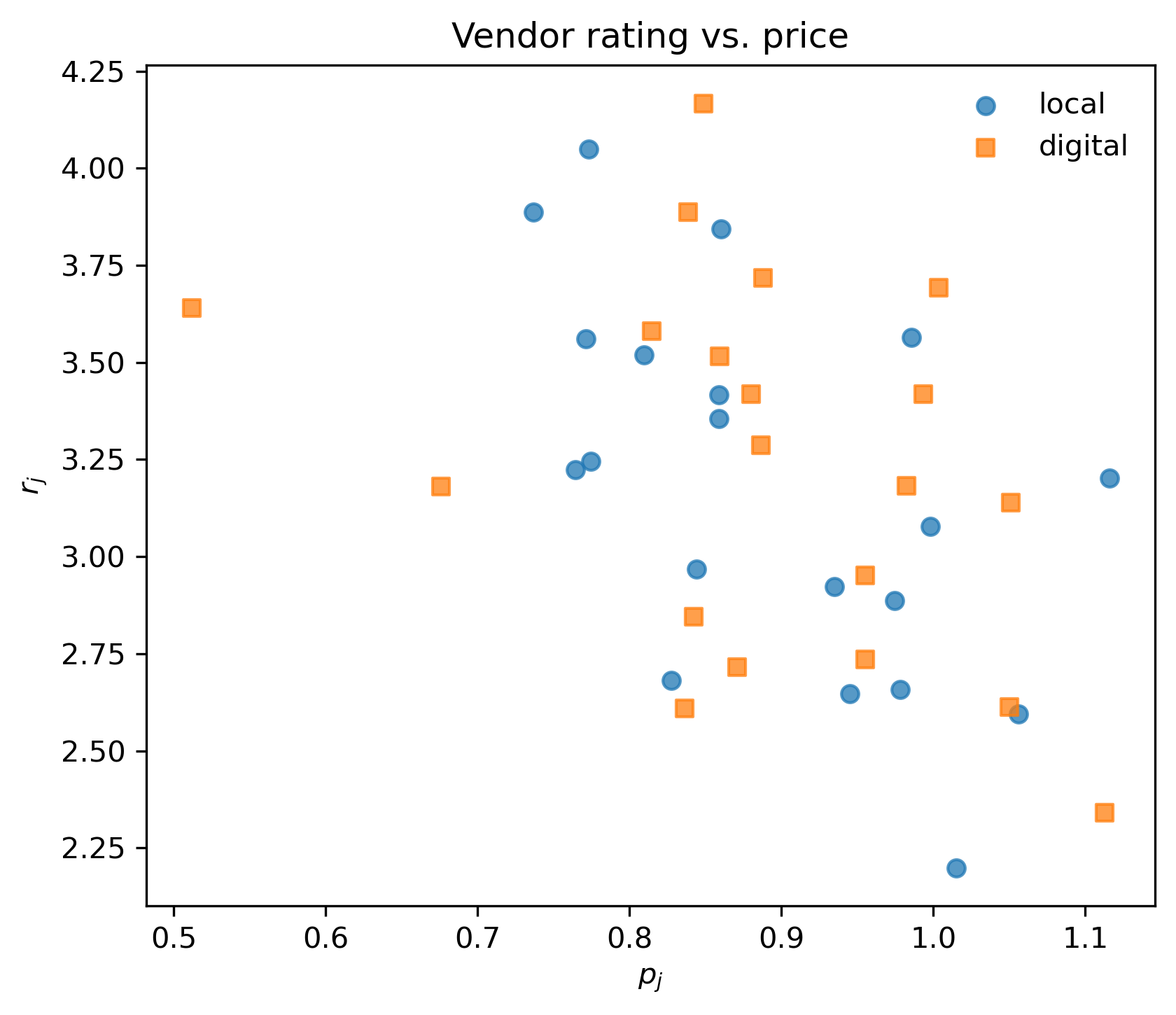
Agents are synthetic. Each run contains N customers and M vendors placed uniformly at random in a unit-square geography (Appendix Fig. 4). Customers have heterogeneous preference parameters, including price sensitivity $\alpha_i$ and delay sensitivity u_i, drawn from fixed distributions with a negative correlation to represent a time–money trade-off: customers who are more price-sensitive tend to be less urgency-sensitive, and vice versa (Appendix Figs. 5–6). Vendors are assigned to be local or digital according to a fixed local fraction, and each vendor is assigned attributes such as price p_j, rating r_j, production cost c_j, and (for digital vendors) a delivery-delay parameter $\tau_j$ (Appendix Figs. 7–8).

Data collection

At each simulation round t, every customer chooses one vendor. We record per-round choice counts $\{n_j(t)\}_{j=1}^{M}$ and compute four summary time series:

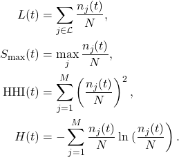
(1) $\begin{align*}L(t) &= \sum_{j\in\mathcal{L}} \frac{n_j(t)}{N}, \\S_{\max}(t) &= \max_j \frac{n_j(t)}{N}, \\\mathrm{HHI}(t) &= \sum_{j=1}^M \left(\frac{n_j(t)}{N}\right)^2, \\H(t) &= -\sum_{j=1}^M \frac{n_j(t)}{N}\ln\!\left(\frac{n_j(t)}{N}\right).\end{align*}$

with the convention that $0\ln 0$ is treated as 0.

Variables and measurements

Choice temperature (T).

Customer choices follow a Boltzmann (softmax) rule, a formalization of stochastic choice that originates in statistical mechanics and has been extensively applied in discrete choice economics.²⁴^,²⁵ Higher T produces more random exploration—customers pay less attention to utility differences—while lower T makes choices more deterministic, so small utility advantages reliably translate into larger market shares.

Information access (γ).

Customers do not initially see every local vendor. Each customer maintains a visibility mask over local vendors. At each round, with probability γ, a customer discovers additional local vendors, with discovery biased toward geographically closer vendors. This setup captures the real-world observation that local sellers are systematically less discoverable than large digital platforms, and that exposure accumulates gradually through proximity, word-of-mouth, or search.

Social influence (φ).

A social term increases the utility of vendors with higher popularity in the previous round. This models the tendency of consumers to be influenced by what others are buying—a phenomenon well documented in both economics and sociophysics.¹⁸^,¹⁶ Setting φ=0 removes social influence entirely and serves as an ablation condition to isolate its effect.

Reinforcement and memory.

Customers carry an affinity toward vendors they have chosen before. Affinities can decay geometrically at a rate controlled by AFFINITY_DECAY; repeated purchases increase affinity. This captures brand loyalty and habit formation in a simple but interpretable way.

ONDC-style protocol and distance weight ( $w$ ).

When protocol_enabled=1, an additional distance-weighted mechanism is applied through protocol_distance_weight =w. Conceptually, this represents the kind of proximity-aware discovery that an open digital commerce protocol could provide: nearby vendors are boosted in customers’ effective consideration sets in proportion to w. In our experiments, w is varied in $[0,1]$ . The grids of γ and w used in the experiments below are stylized choices spanning this interpretable interval; they are not calibrations to specific protocol features or empirical deployment data.

Symbol summary.

For reference, the symbols used in this manuscript are: T (choice-noise temperature in the softmax rule), γ (per-round local-vendor discovery rate), φ (social-influence coupling strength), w (ONDC protocol distance weight, when protocol is enabled), $\rho$ (multiplier for the mean digital delivery delay, $\bar{\tau}$ = $\rho$ x 0.521), $\sigma$ (noise scale on digital delivery delays), and AFFINITY_DECAY (multiplicative decay applied to affinities each round; 1.0 is no decay, 0.0 is full reset). Customer-level sensitivities are $\alpha$ _i (price), u_i (urgency / delay), and $\delta$ _i (reinforcement weight). The outcome metrics are the local share L, the Herfindahl–Hirschman Index HHI $\in$ [0, 1], the Shannon entropy H (in nats), and the top-vendor share S_max.

Procedure

Each simulation run proceeds as follows. A run begins by initializing the population: customers and vendors are generated, with positions and attributes drawn using a fixed random seed. Information masks are then initialized so that all digital vendors are visible to every customer, while local-vendor visibility is set according to the run configuration. The simulation then iterates purchase rounds t = 1, $\dots$ , R. Each round consists of four steps applied in sequence. First, an information update: with probability γ, the local-vendor visibility mask is extended by adding newly discovered local vendors, with discovery biased toward geographically closer vendors. Second, utility computation: utilities U_ij(t) are computed for every visible customer–vendor pair (i,j). Third, stochastic choice: utilities are converted into choice probabilities via a softmax rule and one vendor is sampled for each customer. Fourth, a learning update: customer affinities are updated based on the chosen vendor, and affinity decay is applied if enabled. After all rounds complete, late-time outcomes are computed by averaging L(t), HHI(t), H(t), and S_max(t) over a fixed late-time window to obtain the reported “late” metrics.

Utility model.

We use a linear utility function combining vendor attributes, customer-specific sensitivities, reinforcement, and social influence.²⁶^,²⁷ This type of model, sometimes called a random utility model, assumes that each customer chooses the vendor that provides the highest utility, where utility is the sum of observable attributes (price, rating, delay) and an idiosyncratic noise term. The specific form used here is:

(2) $\begin{equation*}U_{ij}(t)=-\alpha_i\,\tilde{p}_{ij}+\tilde{r}_{j}-u_i\,\tilde{\tau}_{ij}+\delta_i\,\log(1+A_{ij}(t))+\phi\,\log(1+s_{j}(t-1))+s_i\,\epsilon_{ij}(t),\end{equation*}$

where $s_{j}(t-1)=n_j(t-1)/N$ is the previous-round share, A_ij(t) is the affinity state, and $\epsilon$ _ij(t) is i.i.d. Gaussian noise scaled by s_i. Tildes indicate feature rescaling (e.g., standardization) so that T has a consistent interpretation across runs. In the experiments reported here, the per-customer social-noise scale s_i is set to zero throughout, so the $\epsilon$ _ij(t) term contributes no variance to choice; the entire stochastic component of choice in our runs comes from the softmax temperature T in the choice rule below.

Delay term and geography.

For local vendors, delay $\tau_{ij}$ is proportional to Euclidean distance between customer i and vendor j converted into minutes. This is the key channel through which geographic proximity enters the utility of local vendors—a nearby local seller is penalized less than a distant one, all else equal. For digital vendors, delay is based on the vendor’s delivery parameter $\tau_j$ .

Choice rule.

Given utilities over vendors visible to customer i, the probability of choosing vendor j is

(3) $\begin{equation*}P_{ij}(t)=\frac{\exp\!\left(U_{ij}(t)/T\right)}{\sum_{k\in\mathcal{V}_i(t)} \exp\!\left(U_{ik}(t)/T\right)},\end{equation*}$

where V_i(t) is the current consideration set. This softmax rule, equivalent to the Boltzmann distribution in physics, is the standard formulation in the discrete choice literature for modeling stochastic preferences.¹⁵^,²⁵

Data analysis

For each parameter setting, we run multiple independent repeats and report mean late-time outcomes. Where applicable, we compute finite-difference sensitivities of late local share L:

(4) $\begin{equation*}\chi_T \approx \frac{L(T+\Delta T,\gamma)-L(T-\Delta T,\gamma)}{2\Delta T},\qquad\chi_\gamma \approx \frac{L(T,\gamma+\Delta \gamma)-L(T,\gamma-\Delta \gamma)}{2\Delta \gamma},\end{equation*}$

using one-sided differences at grid boundaries. Large values of $\chi_T$ or $\chi_\gamma$ at a particular operating point indicate that the system is in a sensitive region of parameter space—analogous to high susceptibility near a physical phase transition.

Ethical considerations

All agents and data are synthetic; no human participants, personal data, identifiable information, or real transaction data were used in this study. The model is intended as a stylized exploration of mechanisms rather than as a prescription for any specific market or policy outcome.

Data and code availability

The complete simulation code, sweep configuration files, and raw output CSVs underlying every table in this manuscript are publicly available at https://github.com/Amagcodes/vendor-network-abm, along with a README documenting the full parameter specification, the per-job seed propagation scheme (a deterministic function of BASE_SEED=42, the population scenario hash, the repeat index, and the sweep parameter tuple), and a step-by-step reproduction guide. All experiments reported here used BASE_SEED=42, 10 seeds per parameter combination, and 200 simulation rounds unless otherwise noted. Readers can clone the repository, install the dependencies listed in requirements.txt, and reproduce any reported table by invoking the corresponding sweep JSON via the documented run_sim.py CLI.

Results

Baseline with ONDC protocol disabled

We first characterize the baseline model with the ONDC-style protocol turned off (protocol_enabled=0). Unless stated otherwise, all “late” metrics are averages over the final five rounds.

Run configuration (fixed across all repeats): N=200 customers, M=40 vendors, local_fraction =0.5, T=0.5, γ=0.3, φ=0.2, rounds =200, $\rho=1.2$ , $\sigma=0.20$ , affinity_decay =1.0, protocol_distance_weight =0.35. We ran 10 independent repeats.

Table 1 reports mean $\pm$ standard deviation across repeats. Figure 1 shows a representative equilibration trajectory: aggregate metrics settle quickly and then fluctuate weakly around a steady level. The high Herfindahl–Hirschman Index (HHI, $\approx$ 0.64) and top-vendor share ( $\approx$ 0.79) in this baseline confirm that without any discovery-enhancing intervention, the market is heavily concentrated in favor of a small number of vendors—in practice, the digital sellers who are always visible.

Metric	Final	Late
Local share	0.172 ± 0.017	0.170 ± 0.017
HHI	0.642 ± 0.026	0.643 ± 0.024
Entropy	0.788 ± 0.055	0.785 ± 0.050
Top-vendor share	0.790 ± 0.019	0.791 ± 0.018

Table 1 | ONDC-off baseline summary (mean $\pm$ s.d. over 10 runs). “Late” metrics are averages over the last five rounds. HHI is on the $[0, 1]$ scale; entropy is in nats.

*Figure 1 |* Representative equilibration time series for the ONDC-off baseline (T=0.5, γ=0.3, φ=0.2).

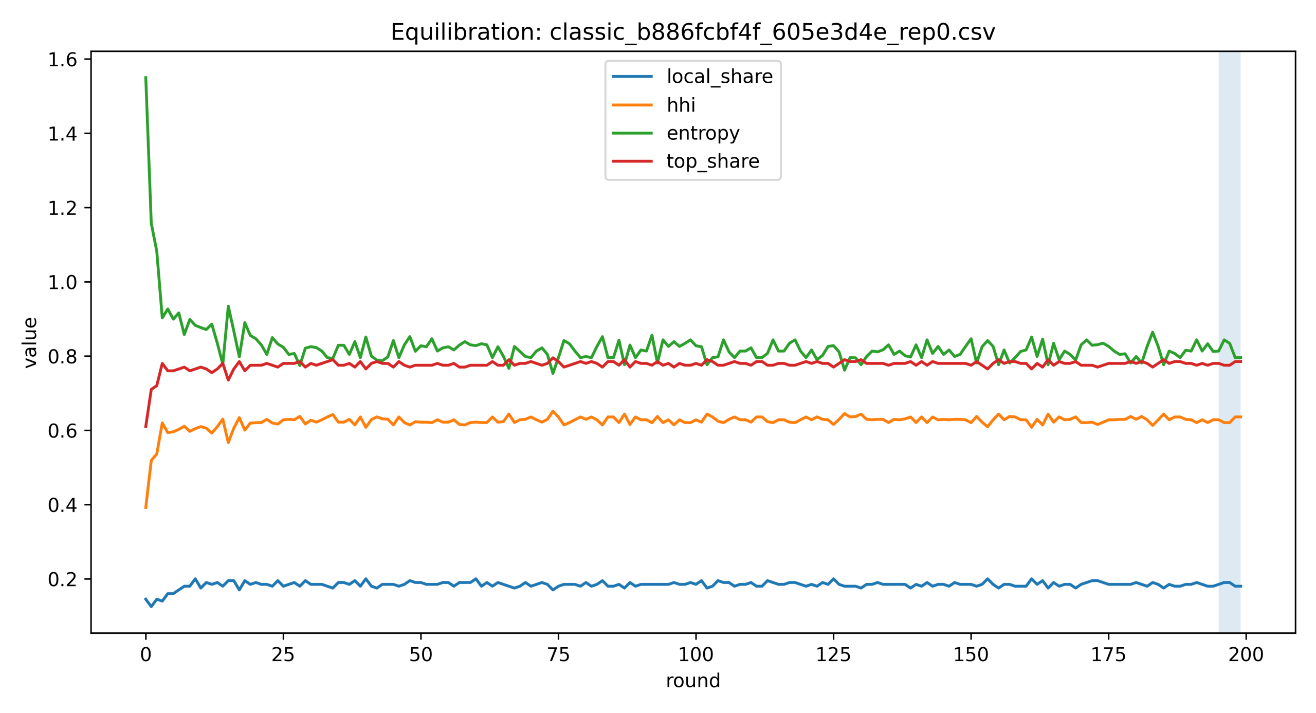
Susceptibility of late local share to T and γ.

The finite-difference sensitivities $\chi_T$ and $\chi_\gamma$ , defined in Methods, quantify how strongly late local share responds to small changes in choice noise and discovery rate at a given operating point. Table 2 reports both quantities at a 3×3 subgrid around the reference baseline (T=0.5, γ=0.3), computed from the per-seed runs that underlie the baseline summary.

T	γ	χ_T	χ_γ
0.2	0.2	+0.06 ± 0.27	+0.62 ± 0.20
0.2	0.3	-0.03 ± 0.24	+0.33 ± 0.28
0.2	0.4	-0.08 ± 0.20	+0.25 ± 0.38
0.5	0.2	+0.14 ± 0.10	+0.31 ± 0.26
0.5	0.3	+0.08 ± 0.17	+0.36 ± 0.33
0.5	0.4	+0.04 ± 0.17	+0.19 ± 0.26
0.7	0.2	+0.18 ± 0.21	+0.36 ± 0.32
0.7	0.3	+0.20 ± 0.22	+0.37 ± 0.37
0.7	0.4	+0.26 ± 0.21	+0.13 ± 0.20

Table 2 | Finite-difference sensitivities $\chi_T$ and $\chi_\gamma$ of late local share at a $3\times3$ subgrid around the reference baseline. Values are mean $\pm$ s.d. across 10 seeds, computed from per-seed late local share by the discrete gradients defined in Methods. All runs use φ=0.2, ONDC protocol disabled, 200 rounds. Cells where $|$ mean $|$ is smaller than the standard deviation should be read as consistent with zero.

Two patterns stand out despite substantial seed-to-seed noise in these finite-difference estimates. First, $\chi_\gamma$ is positive across the grid and is generally larger in magnitude than $\chi_T$ , meaning that late local share responds more strongly to small changes in discovery rate than to small changes in choice noise in this region of parameter space. Second, $\chi_\gamma$ tends to be largest at low γ, where each additional unit of discovery brings in many newly-visible local vendors and the marginal effect on local share is largest. Once a substantial fraction of locals is already discoverable, the marginal value of additional discovery falls.

Vendor attributes in the sampled population.

Locals and digitals are nearly indistinguishable on the exogenous attributes that enter the utility function. Across the cached baseline draw of M=40 vendors, mean price ( $\approx$ 0.89), mean rating ( $\approx$ 3.2), and mean production cost ( $\approx$ 0.68) are statistically equivalent for the two types (n=20 per type; all differences within one standard deviation). The structural asymmetry is entirely in the delay term: digital vendors carry a uniform delivery delay drawn from N( $\rho$ x 0.521, $\sigma^2$ ) with $\rho$ =1.2 and $\sigma$ =0.20 (mean $\approx$ 0.61), while local-vendor delay is the per-customer Euclidean distance to that vendor (mean across all customer–vendor pairs $\approx$ 0.52). The ONDC distance-weight effect (Table 3) therefore operates through the proximity channel alone, not through any systematic price or rating advantage; the protocol amplifies the proximity advantage already present in the delay term, boosting locals that happen to be geographically close to each customer and de-emphasizing locals that are far.

Stationarity of the late-time window.

We checked stationarity at the baseline by comparing the last-5, last-10, and last-20 averages for a representative seed; the three agree to within $\pm$ 0.005 on every metric (local share: 0.185, 0.184, 0.184; HHI: 0.628, 0.627, 0.629; entropy: 0.816, 0.820, 0.815; top share: 0.780, 0.779, 0.780).

Protocol-enabled results (ONDC on)

We next enable the ONDC-style protocol (protocol_enabled=1) and vary the protocol distance-weight parameter w $\in[0,1]$ (protocol_distance_weight). In this implementation, w controls how strongly geographic proximity is emphasized by the protocol mechanism.

Effect of distance weight w at fixed (T,γ,φ).

At fixed T=0.5, γ=0.3, and φ=0.2, increasing w produces higher late-time local share and lower market concentration (HHI and top share), alongside higher entropy (Table 3). The w=0 condition matches the ONDC-off baseline in Table 1, consistent with the protocol having no effect when its distance weighting is inactive. As w increases from 0 to 1, late local share more than triples (from $\approx$ 0.17 to $\approx$ 0.55), HHI roughly halves (from $\approx$ 0.64 to $\approx$ 0.30), top-vendor share falls by nearly half (from $\approx$ 0.79 to $\approx$ 0.44), and entropy nearly doubles—a substantial shift in market structure driven entirely by a change in how proximity is weighted in vendor recommendations.

w	Late local share	Late HHI	Late entropy	Late top share
0.00	0.170 ± 0.017	0.643 ± 0.024	0.785 ± 0.050	0.791 ± 0.018
0.35	0.350 ± 0.028	0.465 ± 0.030	1.098 ± 0.055	0.648 ± 0.028
0.70	0.481 ± 0.021	0.347 ± 0.016	1.329 ± 0.036	0.518 ± 0.022
1.00	0.554 ± 0.019	0.299 ± 0.010	1.436 ± 0.028	0.445 ± 0.019

Table 3 | ONDC-enabled distance-weight sweep at T=0.5, γ=0.3, φ=0.2 (mean $\pm$ s.d. over 10 runs). HHI is on the [0, 1] scale; entropy is in nats.

Representative comparison (ONDC off vs. ONDC on).

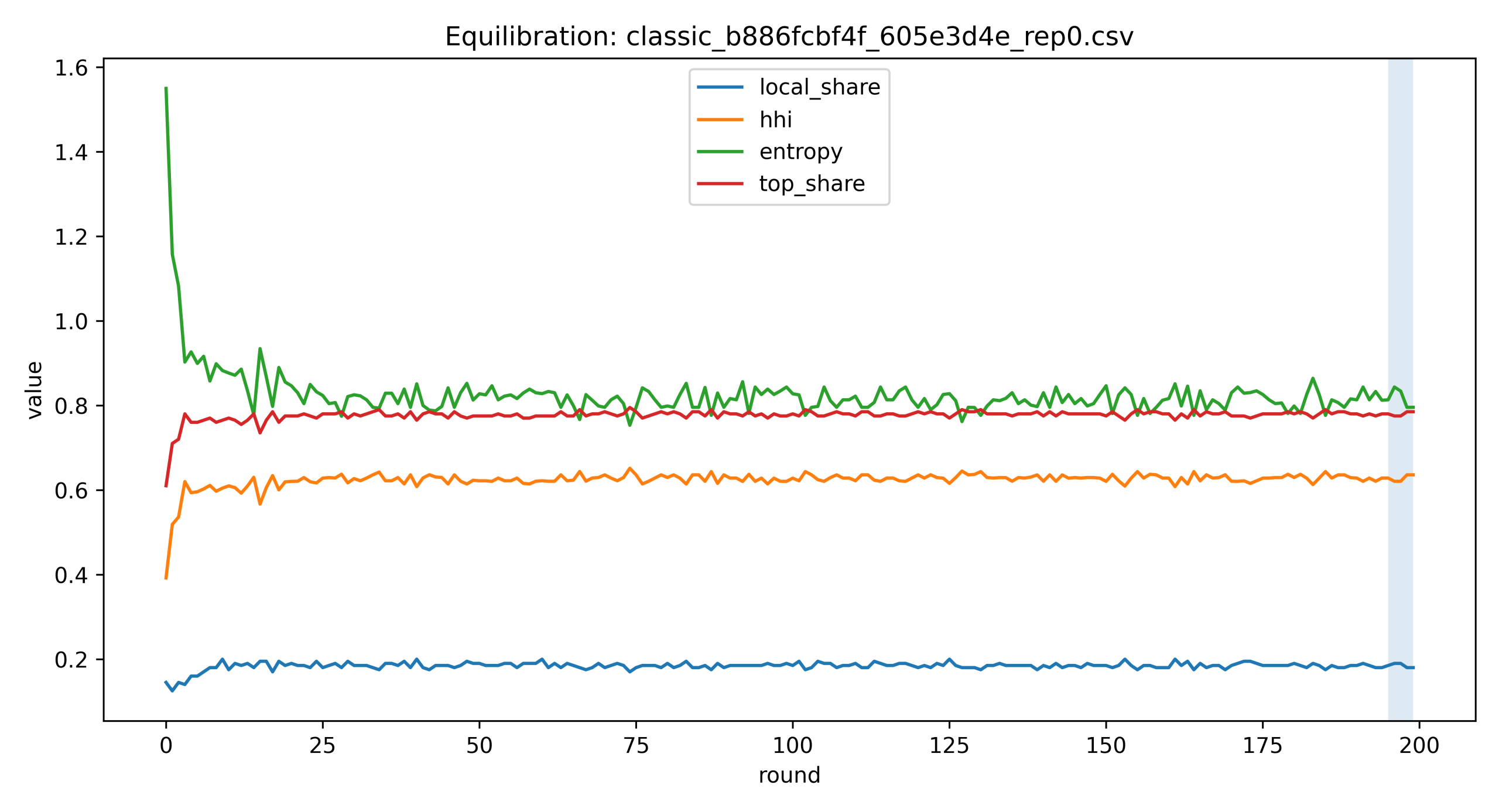
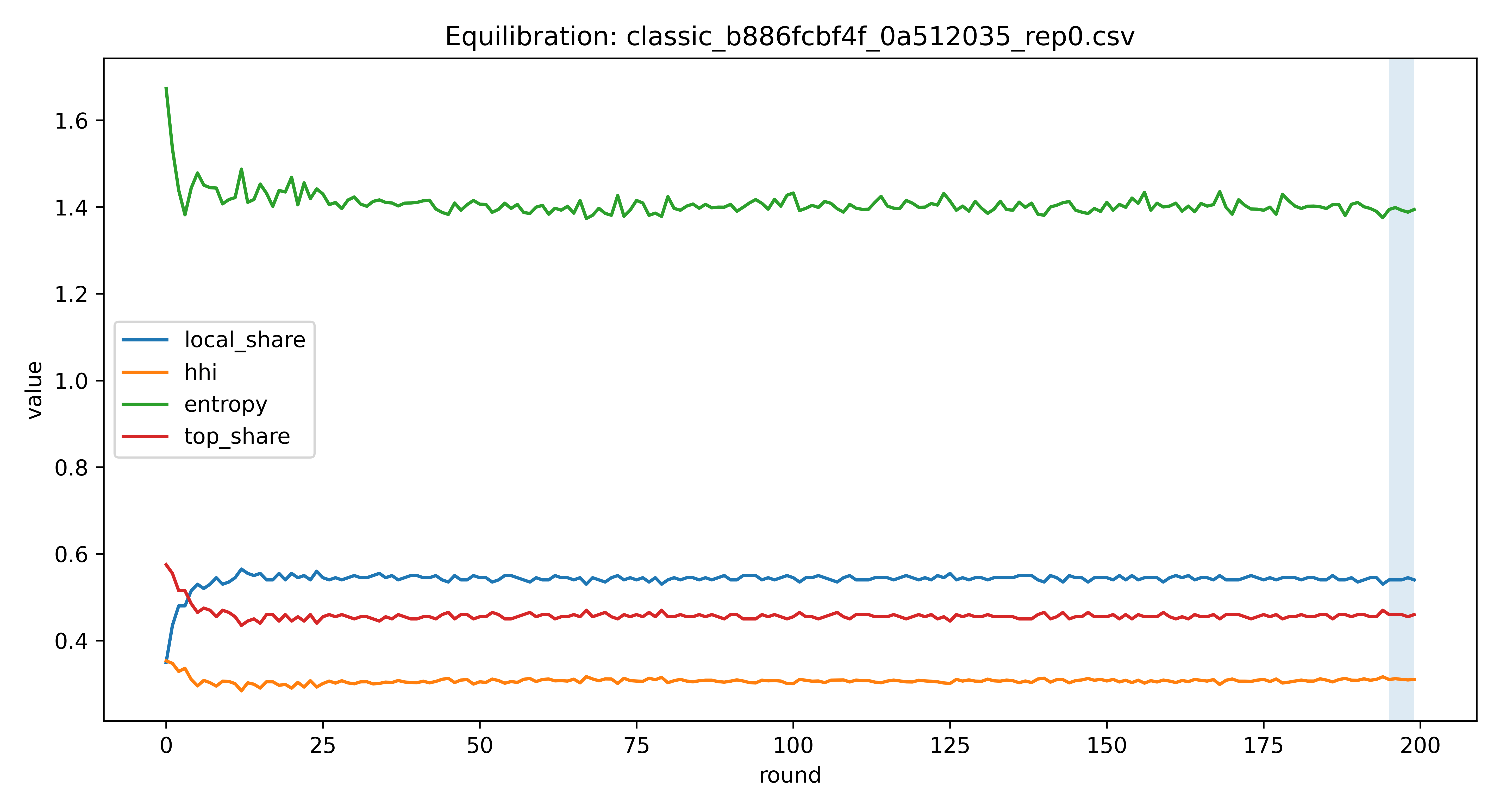
Figure 2 contrasts a representative ONDC-off trajectory with a representative ONDC-on trajectory at high w. The ONDC-on setting shows higher local share and lower concentration relative to the ONDC-off baseline, with the difference visible from early rounds onward.

*Figure 2* | Representative equilibration trajectories with the ONDC-style protocol disabled vs. enabled.

Statistical significance of headline contrasts.

Paired t-tests on per-seed late local share confirm that the four headline contrasts at T=0.5, γ=0.3 are all highly significant (n=10 paired seeds each; p < 0.001 throughout): ONDC w=1.0 vs w=0.0 ( $\Delta$ L = +0.38, Cohen’s d = +22), ONDC on w=0.7 vs off ( $\Delta$ L = +0.31, d = +22), affinity off vs on ( $\Delta$ L = +0.13, d = +8), and φ=0 vs φ=0.2 ( $\Delta$ L = +0.09, d = +4). The large d values reflect the model’s determinism conditional on seed: per-seed standard deviations are small relative to between-condition mean differences.

Interaction slice: information access γ $\times$ distance weight w at fixed (T)

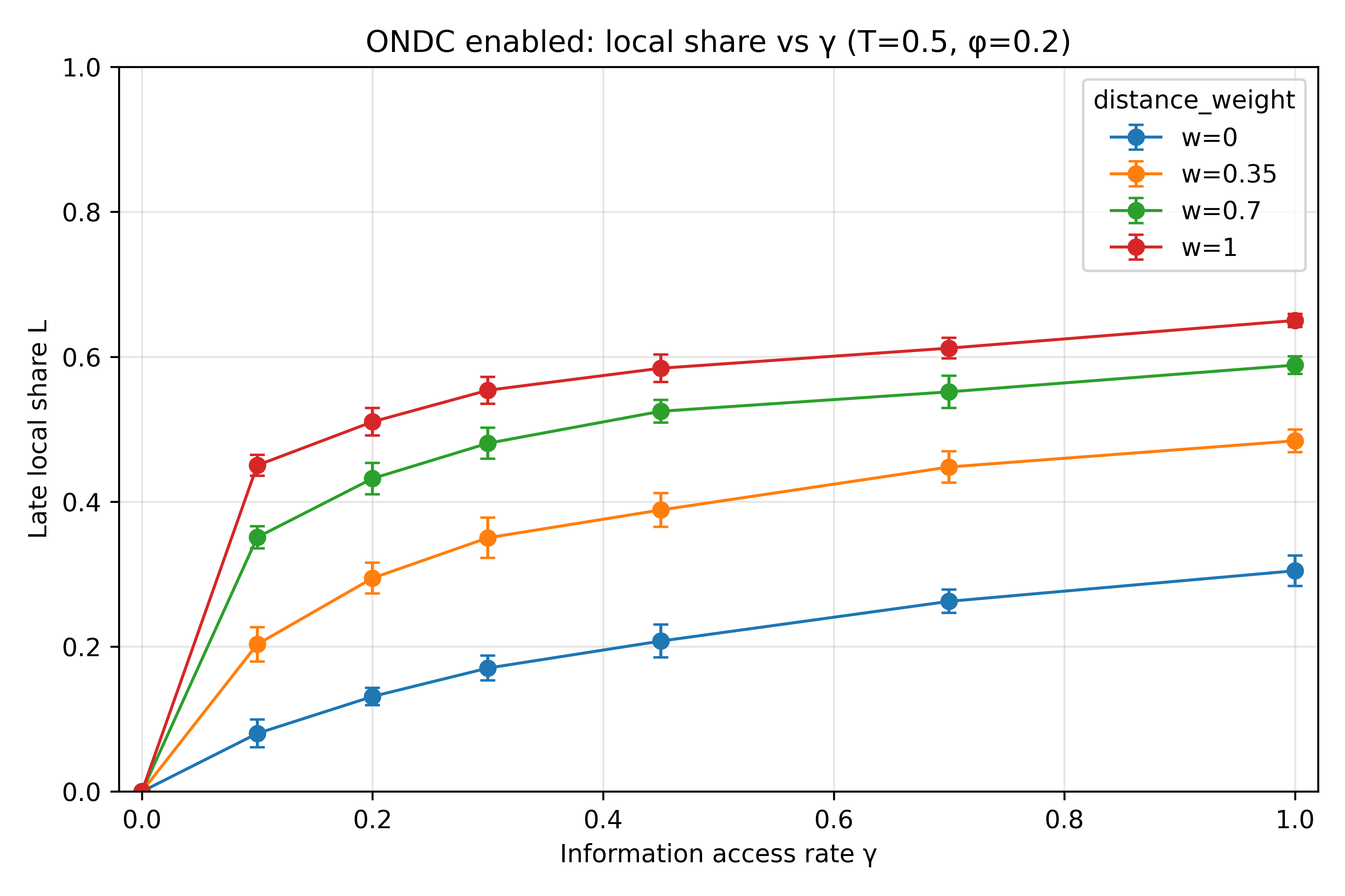
To test whether ONDC primarily behaves like a change in local-vendor visibility, we varied the discovery rate γ together with the protocol distance weight w at fixed T=0.5 and φ=0.2. The full grid of late local share values (mean $\pm$ s.d. across 10 runs per setting) is reported in Appendix Table 7.

Two descriptive patterns follow directly from the grid. By construction, when γ = 0, local vendors are never discovered and the late local share is zero for all w; this acts as a visibility gate. Once locals are discoverable, for γ > 0, the late local share varies substantially with w, including at γ = 1.

Figure 3 provides one visualization of this interaction slice.

*Figure 3 |* ONDC-on interaction slice at fixed T=0.5 and φ=0.2. Late local share is shown across the γ x w sweep. Each curve corresponds to a different distance weight w; error bars show standard deviation across 10 runs.

Behavioural ablations: social influence and reinforcement

Social-influence ablation (φ=0 vs. φ=0.2).

To isolate the contribution of social influence to aggregate market structure, we re-ran the baseline with φ set to zero. Table 4 reports late local share and HHI for a 3 x 4 grid of (T, γ) values comparing the baseline (φ=0.2) with the ablation (φ=0). All other parameters are held fixed, the ONDC-style protocol is disabled, and each cell averages over 10 independent seeds at 200 rounds.

		Local share L		HHI
T	γ	φ=0.2	φ=0	φ=0.2	φ=0
0.3	0.25	0.131 ± 0.022	0.200 ± 0.026	0.658 ± 0.022	0.520 ± 0.030
0.3	0.30	0.154 ± 0.024	0.224 ± 0.021	0.644 ± 0.043	0.509 ± 0.022
0.3	0.35	0.176 ± 0.025	0.237 ± 0.015	0.619 ± 0.025	0.503 ± 0.015
0.3	0.40	0.185 ± 0.020	0.246 ± 0.016	0.605 ± 0.027	0.502 ± 0.017
0.5	0.25	0.152 ± 0.017	0.246 ± 0.013	0.652 ± 0.015	0.482 ± 0.024
0.5	0.30	0.170 ± 0.017	0.263 ± 0.015	0.643 ± 0.024	0.477 ± 0.018
0.5	0.35	0.189 ± 0.021	0.277 ± 0.025	0.619 ± 0.020	0.463 ± 0.023
0.5	0.40	0.200 ± 0.021	0.284 ± 0.017	0.598 ± 0.026	0.464 ± 0.027
0.7	0.25	0.176 ± 0.022	0.287 ± 0.022	0.636 ± 0.024	0.454 ± 0.019
0.7	0.30	0.196 ± 0.015	0.311 ± 0.014	0.625 ± 0.024	0.431 ± 0.020
0.7	0.35	0.213 ± 0.022	0.321 ± 0.014	0.598 ± 0.021	0.428 ± 0.017
0.7	0.40	0.227 ± 0.020	0.323 ± 0.016	0.592 ± 0.017	0.429 ± 0.016

Table 4 | Social-influence ablation. Late local share L and Herfindahl–Hirschman Index (on the [0, 1] scale) over a 3 $\times$ 4 grid of (T,γ) at φ=0.2 (baseline) versus φ=0 (ablation). All runs use ONDC protocol disabled, φ=1.2, $\sigma$ =0.20, 200 rounds, 10 seeds. Values reported as mean $\pm$ s.d. across seeds.

Removing social influence shifts both metrics toward less concentration. At the reference baseline (T=0.5, γ=0.3), late local share rises from 0.170 $\pm$ 0.017 to 0.263 $\pm$ 0.015 and HHI falls from 0.643 $\pm$ 0.024 to 0.477 $\pm$ 0.018. The direction is the same at every cell of the grid: φ=0 gives higher local share and lower HHI than φ=0.2 at all twelve (T,γ) combinations, with the change in local share ranging from about 0.06 to 0.11. Two points follow. First, the social-influence term contributes substantially to baseline concentration: at the reference cell, removing it closes roughly half of the gap between the baseline local share and the local-vendor population fraction of 0.5. Second, the size of the φ effect varies modestly with T and γ, but the direction is the same at every operating point, suggesting that social influence adds to concentration roughly independently of the other two parameters.

Reinforcement ablation (AFFINITY_DECAY=0 vs. baseline).

To isolate the contribution of the affinity/reinforcement mechanism, we re-ran the model with the affinity decay factor set to zero. This clears the affinity matrix at the start of each round and prevents accumulated preference for previously-chosen vendors from carrying across purchases. Table 5 reports late local share and HHI across the seven γ values used in the discovery-rate sweep, comparing the baseline (AFFINITY_DECAY=1.0; no decay) with the ablation (AFFINITY_DECAY=0.0; full reset each round). All other parameters are held at their baseline values, the ONDC-style protocol is disabled, T=0.5, φ=0.2, and each cell averages over 10 seeds at 200 rounds.

	Local share L		HHI
γ	baseline	affinity off	baseline	affinity off
0.00	0.000 ± 0.000	0.000 ± 0.000	0.797 ± 0.024	0.775 ± 0.019
0.10	0.080 ± 0.019	0.313 ± 0.020	0.713 ± 0.031	0.486 ± 0.019
0.20	0.131 ± 0.012	0.295 ± 0.024	0.665 ± 0.028	0.501 ± 0.023
0.30	0.170 ± 0.017	0.296 ± 0.015	0.643 ± 0.024	0.488 ± 0.012
0.45	0.208 ± 0.023	0.298 ± 0.015	0.608 ± 0.031	0.503 ± 0.016
0.70	0.263 ± 0.016	0.293 ± 0.017	0.554 ± 0.025	0.505 ± 0.025
1.00	0.305 ± 0.021	0.296 ± 0.015	0.513 ± 0.021	0.496 ± 0.017

Table 5 | Reinforcement ablation. Late local share L and Herfindahl–Hirschman Index (on the [0, 1] scale) across seven γ values comparing the baseline (AFFINITY_DECAY=1.0; full reinforcement persistence) with the ablation (AFFINITY_DECAY=0.0; affinity reset each round). All runs use T=0.5, φ=0.2, ONDC protocol disabled, $\rho$ =1.2, $\sigma$ =0.20, 200 rounds, 10 seeds. Values reported as mean $\pm$ s.d. across seeds.

Two patterns emerge. First, at every γ value tested, removing reinforcement raises local share and lowers HHI relative to the baseline, with the gain in local share ranging from about 0.23 at γ=0.10 down to about 0.01 at γ=1.00. Second, the affinity-off local share is essentially flat across γ $\ge$ 0.10 (all values within 0.02 of one another), whereas the baseline local share rises monotonically from 0.080 at γ=0.10 to 0.305 at γ=1.00. The interpretation is that reinforcement amplifies path dependence in this model: in the baseline, early-round choices made before locals are well-discovered get carried forward through accumulated affinity, so low discovery rates trap the market in low-local-share states. Once reinforcement is removed, the choice rule is effectively memoryless across rounds and the system equilibrates to a similar local share regardless of how quickly locals were discovered. The same direction of effect holds when the ONDC-style protocol is enabled: at γ=0.3 with w=0.7, late local share is 0.481 $\pm$ 0.021 with reinforcement and 0.605 $\pm$ 0.017 without, indicating that the protocol mechanism operates independently of the reinforcement channel.

Sensitivity to choice noise T.

To assess the noise-axis robustness of the ONDC effect, we swept T $\in$ {0.10, 0.15, 0.20, 0.25, 0.30, 0.40, 0.50, 0.60, 0.70} at the reference baseline (γ=0.3, φ=0.2, ONDC off). Table 6 reports the late metrics; Appendix Table 8 reports the full 9 x 9 T γ grid of L. The T effect on local share is real but small: across the range, L at γ=0.3 varies between 0.137 and 0.196 (a swing of $\approx$ 0.06), and HHI and top-share each move less than 0.03. By comparison at the same operating point, moving w from 0 to 1 raises L by approximately +0.38 (Table 3), removing reinforcement raises it by +0.13 (Table 5), and removing social influence raises it by +0.09 (Table 4). The ONDC effect therefore persists across the choice-noise range studied; T is the smallest of the four behavioural channels in terms of its absolute effect on L.

T	L	HHI	top share	entropy
0.10	0.153 ± 0.021	0.628 ± 0.029	0.784 ± 0.019	0.863 ± 0.072
0.15	0.145 ± 0.019	0.638 ± 0.022	0.791 ± 0.015	0.834 ± 0.048
0.20	0.137 ± 0.014	0.641 ± 0.032	0.792 ± 0.022	0.821 ± 0.069
0.25	0.142 ± 0.016	0.641 ± 0.024	0.793 ± 0.016	0.822 ± 0.061
0.30	0.154 ± 0.024	0.644 ± 0.043	0.793 ± 0.030	0.812 ± 0.095
0.40	0.160 ± 0.024	0.647 ± 0.023	0.794 ± 0.016	0.781 ± 0.060
0.50	0.170 ± 0.017	0.643 ± 0.024	0.791 ± 0.018	0.785 ± 0.050
0.60	0.176 ± 0.017	0.635 ± 0.023	0.784 ± 0.016	0.796 ± 0.061
0.70	0.196 ± 0.015	0.625 ± 0.024	0.774 ± 0.018	0.784 ± 0.053

Table 6 | Sensitivity of late local share, HHI, top-vendor share, and entropy to choice-noise temperature T at the reference baseline (γ=0.3, φ=0.2, ONDC off, 200 rounds, 10 seeds). Values reported as mean $\pm$ s.d. across seeds. HHI is on the [0, 1] scale; entropy is in nats.

Discussion

Across these experiments, the information-access parameter γ functions as a strict gate for local participation: when γ=0, local vendors remain invisible and receive zero purchases by construction, regardless of any protocol settings (Appendix Table 7). This result underscores a point that is easy to overlook in policy discussions—no amount of proximity weighting or protocol design can benefit local sellers who are never discovered in the first place. Visibility itself is a necessary precondition for competition, not just an advantage once competition is established.

For γ>0, enabling the ONDC-style protocol and increasing the distance weight w is consistently associated with higher late local share and lower concentration, as reflected in Table 3. The magnitude of this effect is notable: moving from w=0 to w=1 at γ=0.3 more than triples the local share, from approximately 0.17 to 0.55, while roughly halving the HHI from 0.64 to 0.30. This is a large change in market structure induced purely by shifting the weight placed on geographic proximity in the discovery mechanism, without any change to vendor prices, ratings, or other attributes.

The interaction slice further shows that w continues to modulate outcomes even under full discovery (γ=1), indicating that the protocol effect is not simply about making locals visible—it also matters how strongly geographic proximity is weighted once locals are in the consideration set. In terms of the model’s structure, this confirms that γ and w operate through distinct channels: γ determines whether a vendor enters the customer’s consideration set at all, while w adjusts how attractive nearby vendors appear once they are there.

This study is limited by its stylized design: vendor attributes are fixed random draws, customers follow a simplified utility model, and vendor-side strategy (e.g., pricing responses to new competition) is not included. These are meaningful simplifications, and the absence of vendor-side strategic response is in particular a central rather than peripheral limitation, since any extension of this work to long-run market-structure claims would need to incorporate such dynamics. The model also uses a single market size (N=200 customers, M=40 vendors at 50% local fraction) and a linear-in-attributes utility specification; a systematic robustness sweep over these structural parameters and a comparison against alternative functional forms (e.g., nonlinear price scaling or saturating delay penalties) were not run. In a real market, vendors would adjust their prices and marketing in response to changing competition, and customers would have richer preference structures than a linear utility function can capture. Within these constraints, however, the results illustrate how interpretable mechanisms for information access and distance-weighting can correspond to large, consistent changes in aggregate market outcomes. The framework is not meant to predict any specific market precisely, but to isolate and study the mechanisms that real policy interventions engage.

Future work can extend the same framework in several directions: expanding the parameter sweeps to include a broader range of T, testing additional ablations or model variations already described in the Methods (such as varying social influence strength or affinity decay), and incorporating simple forms of vendor-side strategic response. Such extensions would allow a richer exploration of the conditions under which distance-weighted discovery protocols produce robust versus fragile improvements in local-vendor market access.

In short, the model shows how a small set of interpretable controls—visibility, distance-weighting, social influence, and reinforcement—together shape the local-versus-digital balance in a stylized market, with discoverability and proximity-weighting carrying most of the weight in the operating range studied.

Appendix

Appendix: Population and attribute generation

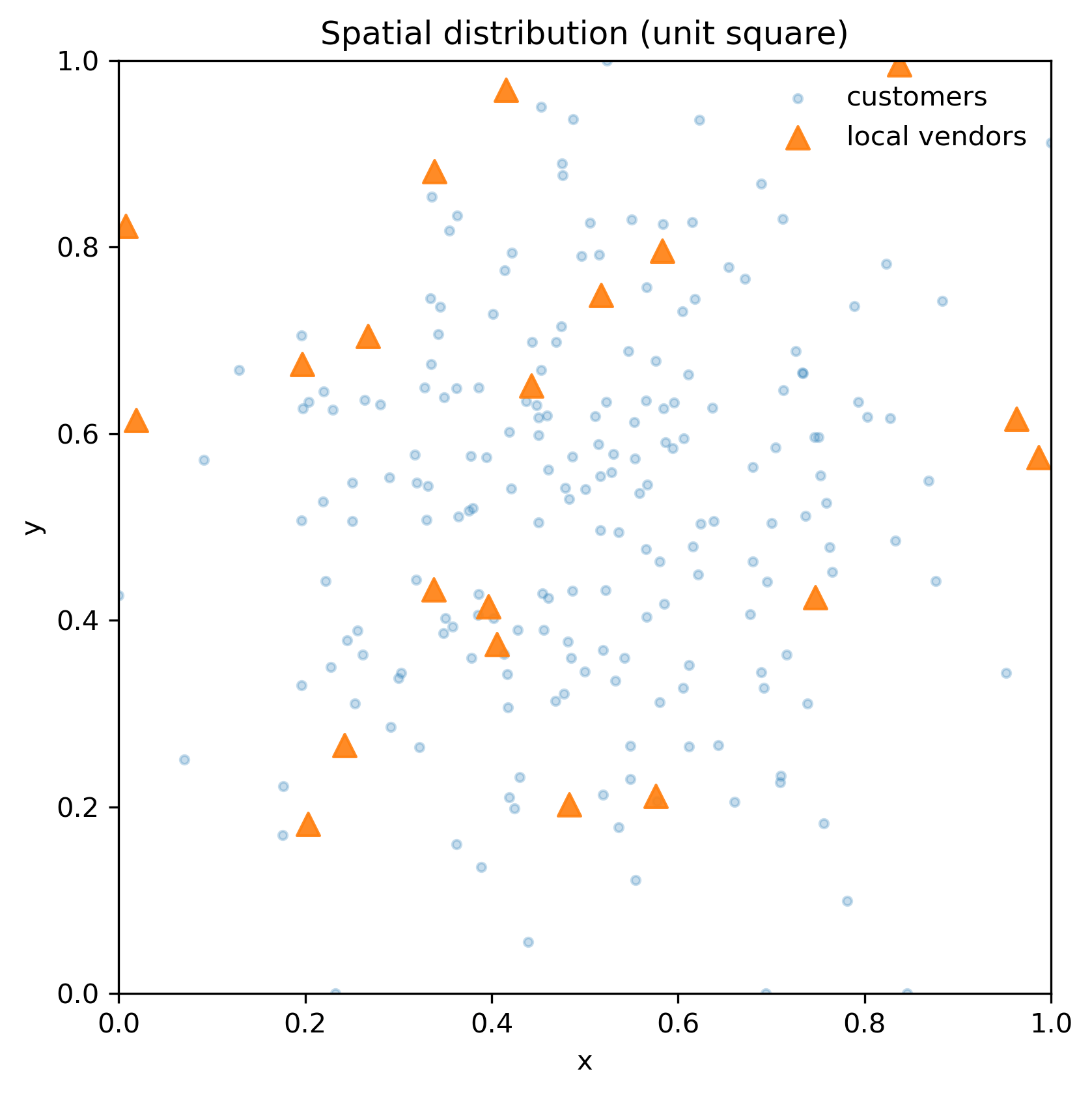
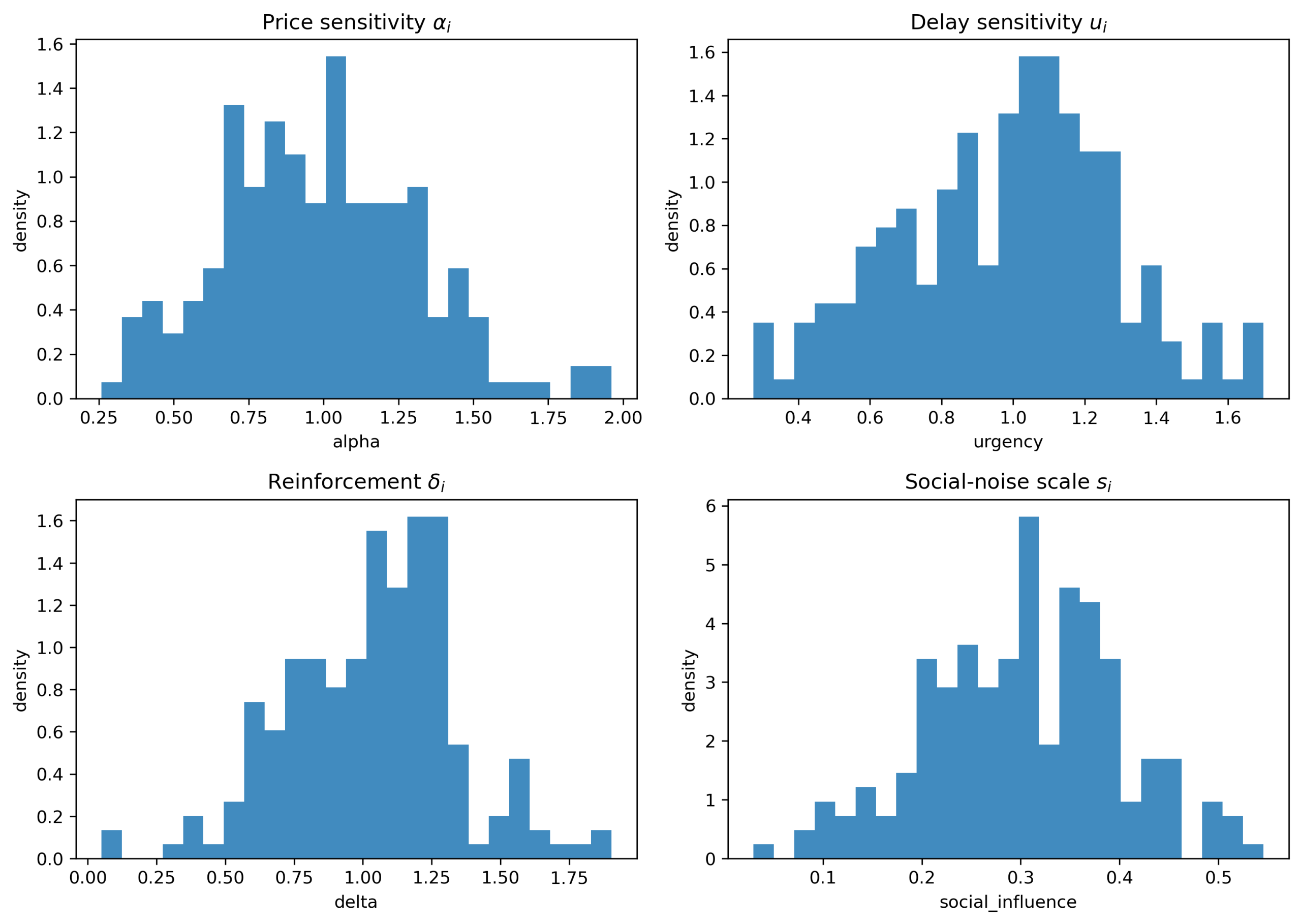
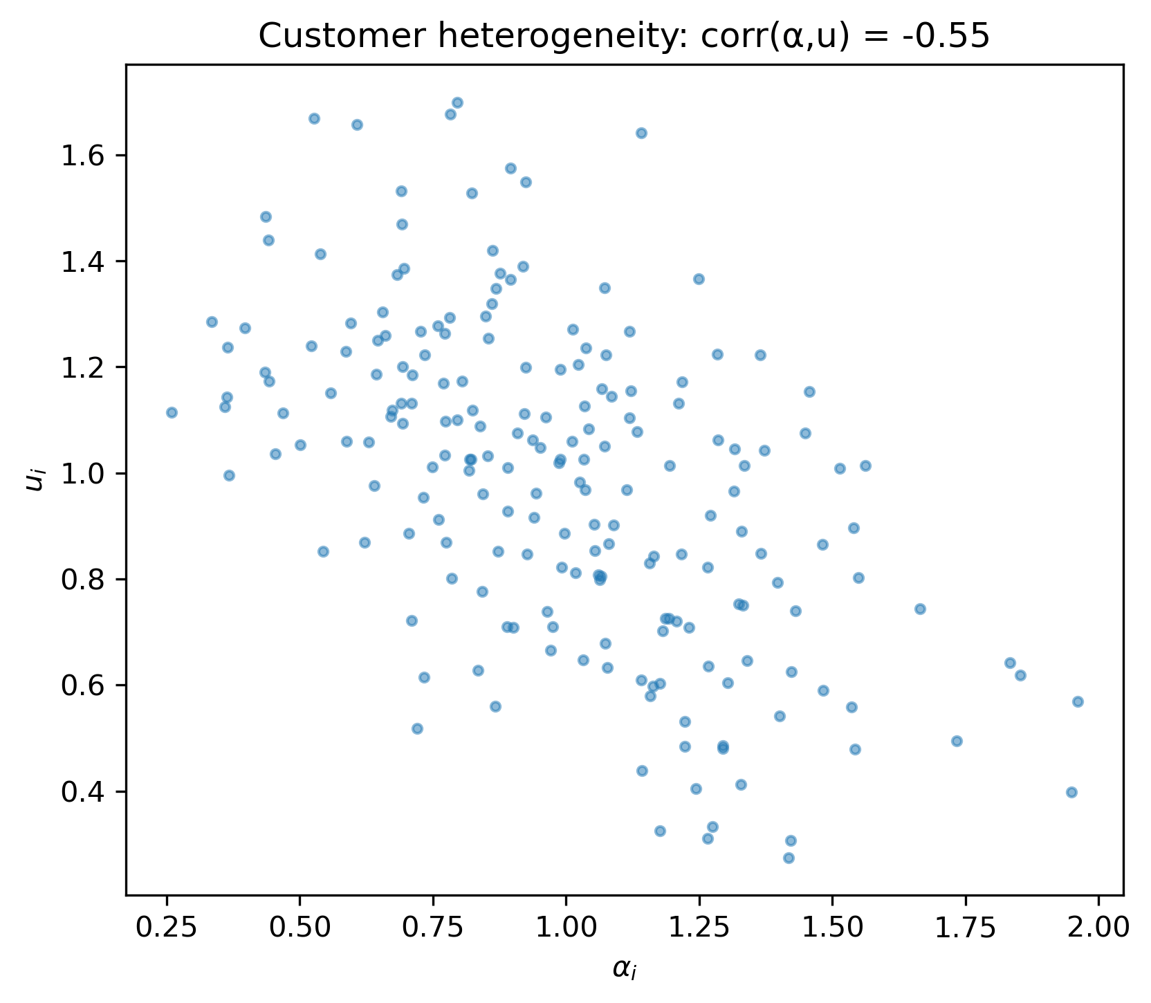
*Figure 4 |* Spatial distribution of customers (points) and local vendors (triangles) in the unit-square geography. Single example draw with N=200 customers and M=40 vendors.

*Figure 5 |* Customer heterogeneity distributions (price sensitivity, delay sensitivity, reinforcement strength, and social-noise scale). Single example draw with N=200 customers.

*Figure 6 |* Joint distribution of $(\alpha_i,u_i)$ showing a negative correlation (time–money trade-off). Single example draw with N=200 customers.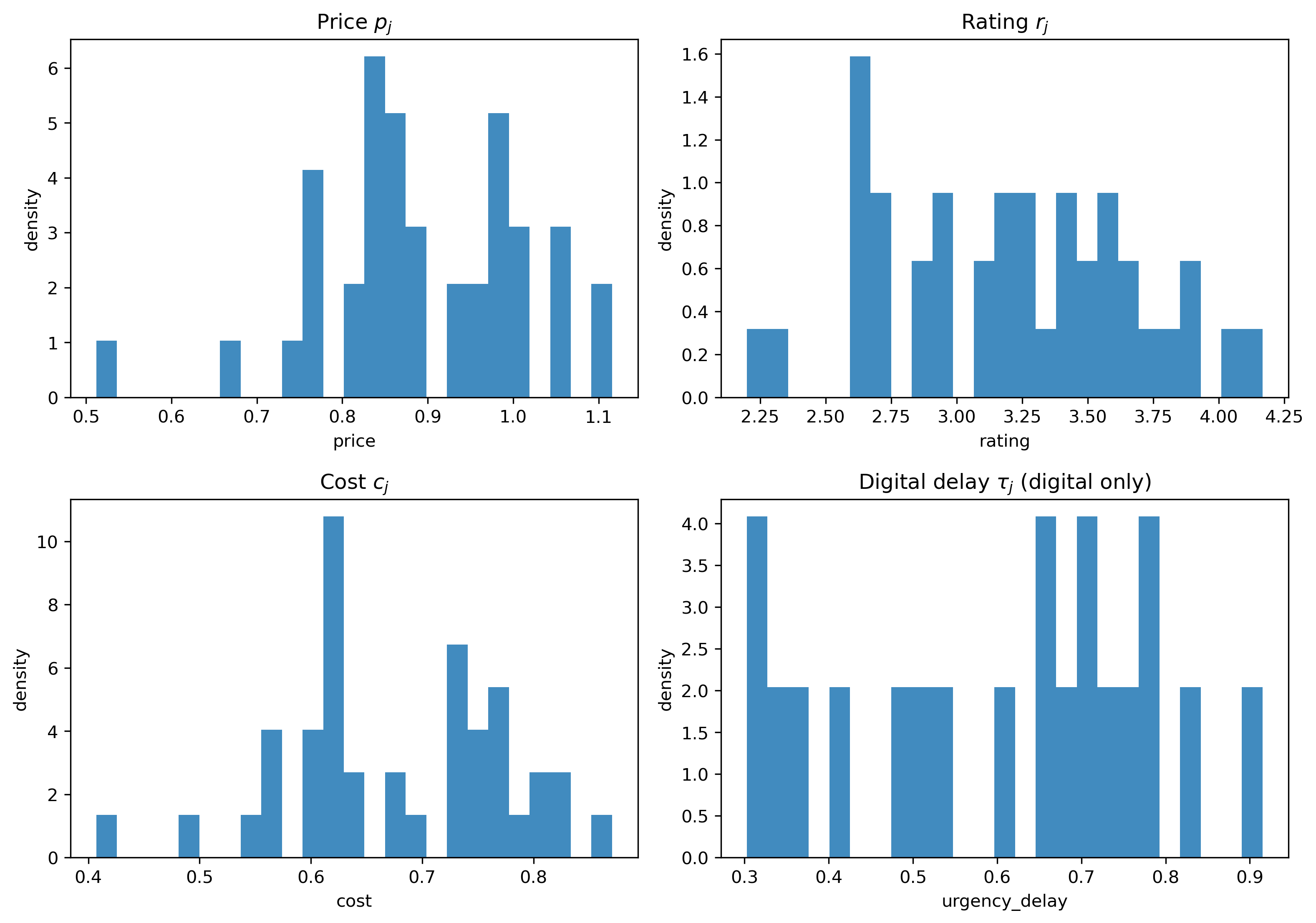

*Figure 7 |* Vendor attribute distributions (price, rating, cost, and a delivery-delay parameter for digital vendors). Single example draw with M=40 vendors at 50% local fraction.

*Figure 8 |* Example scatter of vendor rating versus price, separated by local vs. digital type. Single example draw with M=40 vendors at 50% local fraction.

Appendix: Full ONDC interaction slice

γ	w=0.0	w=0.35	w=0.7	w=1.0
0.00	0.000 ± 0.000	0.000 ± 0.000	0.000 ± 0.000	0.000 ± 0.000
0.10	0.080 ± 0.019	0.203 ± 0.024	0.351 ± 0.015	0.450 ± 0.015
0.20	0.131 ± 0.012	0.295 ± 0.021	0.432 ± 0.022	0.510 ± 0.019
0.30	0.170 ± 0.017	0.350 ± 0.028	0.481 ± 0.021	0.554 ± 0.019
0.45	0.208 ± 0.023	0.389 ± 0.023	0.525 ± 0.016	0.584 ± 0.019
0.70	0.263 ± 0.016	0.448 ± 0.022	0.552 ± 0.022	0.612 ± 0.014
1.00	0.305 ± 0.021	0.484 ± 0.016	0.589 ± 0.012	0.650 ± 0.009

Table 7 | Late local share (mean $\pm$ s.d., 10 runs) for the ONDC-enabled interaction slice at T=0.5, φ=0.2. Columns correspond to ONDC distance weight w.

Appendix: T x γ sweep of late local share

T \ γ	0.10	0.15	0.20	0.25	0.30	0.35	0.40	0.45	0.50
0.10	0.054	0.078	0.106	0.140	0.153	0.169	0.190	0.214	0.226
0.15	0.057	0.080	0.105	0.129	0.145	0.166	0.193	0.201	0.219
0.20	0.060	0.073	0.099	0.136	0.137	0.168	0.190	0.193	0.215
0.25	0.056	0.082	0.111	0.132	0.142	0.166	0.185	0.202	0.207
0.30	0.054	0.084	0.102	0.131	0.154	0.176	0.185	0.195	0.214
0.40	0.072	0.093	0.113	0.147	0.160	0.168	0.193	0.197	0.205
0.50	0.080	0.122	0.131	0.152	0.170	0.189	0.200	0.208	0.214
0.60	0.102	0.112	0.141	0.160	0.176	0.204	0.201	0.219	0.217
0.70	0.122	0.140	0.159	0.176	0.196	0.213	0.227	0.226	0.240

Table 8 | Late local share (mean across 10 seeds per cell) across the full T x γ grid at φ=0.2, ONDC disabled, 200 rounds. Rows index T, columns index γ. Per-cell standard deviations range from 0.010 to 0.028 across the grid; the per-cell s.d. values are available in the public code repository (see Methods, “Data and code availability”).

References

M. L. Katz, C. Shapiro. Network externalities, competition, and compatibility. American Economic Review. Vol. 75, pg. 424–440, 1985. [↩]
J.-C. Rochet, J. Tirole. Platform competition in two-sided markets. Journal of the European Economic Association. Vol. 1, pg. 990–1029, 2003, https://doi.org/10.1162/154247603322493212. [↩]
W. B. Arthur. Competing technologies, increasing returns, and lock-in by historical events. Economic Journal. Vol. 99, pg. 116–131, 1989, https://doi.org/10.2307/2234208. [↩]
E. Brynjolfsson, Y. Hu, M. D. Smith. Consumer surplus in the digital economy: Estimating the value of increased product variety at online booksellers. Management Science. Vol. 49, pg. 1580–1596, 2003, https://doi.org/10.1287/mnsc.49.11.1580.20580. [↩]
S. Bikhchandani, D. Hirshleifer, I. Welch. A theory of fads, fashion, custom, and cultural change as informational cascades. Journal of Political Economy. Vol. 100, pg. 992–1026, 1992, https://doi.org/10.1086/261849. [↩]
A. V. Banerjee. A simple model of herd behavior. Quarterly Journal of Economics. Vol. 107, pg. 797–817, 1992, https://doi.org/10.2307/2118364. [↩]
M. J. Salganik, P. S. Dodds, D. J. Watts. Experimental study of inequality and unpredictability in an artificial cultural market. Science. Vol. 311, pg. 854–856, 2006, https://doi.org/10.1126/science.1121066. [↩]
G. Ellison, S. F. Ellison. Search, obfuscation, and price elasticities on the internet. Econometrica. Vol. 77, pg. 427–452, 2009, https://doi.org/10.3982/ECTA5708. [↩]
C. Castellano, S. Fortunato, V. Loreto. Statistical physics of social dynamics. Reviews of Modern Physics. Vol. 81, pg. 591–646, 2009, https://doi.org/10.1103/RevModPhys.81.591. [↩]
R. N. Mantegna, H. E. Stanley. An introduction to econophysics: Correlations and complexity in finance. Cambridge University Press, 2000. [↩]
T. Lux, M. Marchesi. Scaling and criticality in a stochastic multi-agent model of a financial market. Nature. Vol. 397, pg. 498–500, 1999, https://doi.org/10.1038/17290. [↩]
H. E. Stanley. Introduction to phase transitions and critical phenomena. Oxford University Press, 1971. [↩]
D. Sornette. Critical phenomena in natural sciences: Chaos, fractals, selforganization and disorder. 2nd ed. Springer, 2006. [↩]
T. C. Schelling. Micromotives and macrobehavior. Norton, 1978. [↩]
L. E. Blume. The statistical mechanics of strategic interaction. Games and Economic Behavior. Vol. 5, pg. 387–424, 1993, https://doi.org/10.1006/game.1993.1023. [↩] [↩]
W. A. Brock, S. N. Durlauf. Discrete choice with social interactions. Review of Economic Studies. Vol. 68, pg. 235–260, 2001, https://doi.org/10.1111/1467-937X.00168. [↩] [↩]
S. N. Durlauf. Nonergodic economic growth. Review of Economic Studies. Vol. 60, pg. 349–366, 1993, https://doi.org/10.2307/2298061. [↩]
S. Galam, S. Moscovici. Towards a theory of collective phenomena: Consensus and attitude changes in groups. European Journal of Social Psychology. Vol. 21, pg. 49–74, 1991, https://doi.org/10.1002/ejsp.2420210105. [↩] [↩]
R. Cont, J.-P. Bouchaud. Herd behavior and aggregate fluctuations in financial markets. Macroeconomic Dynamics. Vol. 4, pg. 170–196, 2000, https://doi.org/10.1017/S1365100500015029. [↩]
Department for Promotion of Industry and Internal Trade. Open network for digital commerce: Policy and technical framework. Government of India, New Delhi, 2022. https://ondc.org. [↩]
K. J. Boudreau. Open platform strategies and innovation: Granting access vs. devolving control. Management Science. Vol. 56, pg. 1849–1872, 2010, https://doi.org/10.1287/mnsc.1100.1215. [↩]
J. M. Epstein, R. Axtell. Growing artificial societies: Social science from the bottom up. MIT Press, 1996. [↩]
L. Tesfatsion, K. L. Judd, eds. Handbook of computational economics, volume 2: Agent-based computational economics. Elsevier, 2006. [↩]
K. Huang. Statistical mechanics. 2nd ed. Wiley, 1987. [↩]
D. McFadden. Conditional logit analysis of qualitative choice behavior. In P. Zarembka, ed., Frontiers in econometrics. Academic Press, pg. 105–142, 1974. [↩] [↩]
K. E. Train. Discrete choice methods with simulation. Cambridge University Press, 2003. [↩]
S. P. Anderson, A. de Palma, J.-F. Thisse. Discrete choice theory of product differentiation. MIT Press, 1992. [↩]