Predicting Limited Service Zones Using GIS-Integrated Machine Learning: A Case Study of Three Cities

Abstract

Local businesses are important to neighborhood service access, but access to these services is limited in some areas. This study uses GIS and machine learning to identify possible limited service zones for restaurants and supermarkets across Dublin, Pleasanton, and Livermore in Alameda County, California. The model dataset included 1,134 Alameda County census block groups, each treated as an analysis zone. The three cities were used for interpretation. Each zone was labeled limited service when the selected category, restaurant or supermarket, was allowed by zoning, but no matching business was located inside the zone or in the surrounding 300 m area. Based on this definition, 95 restaurant zones and 318 supermarket zones were labeled as limited service. Logistic Regression, Random Forest, and Gradient Boosting models were trained using neighborhood, parcel, demographic, and accessibility features. To reduce target leakage, business count, business density and zoning allowance features were removed. Model weights addressed class imbalance, and F1 score was the main evaluation metric. Gradient Boosting performed best for restaurants, with accuracy of 0.887 and F1 score 0.315. Random Forest performed best for supermarkets, with accuracy of 0.638 and F1 score 0.518. The predicted zones generally followed the calculated limited service zones, but the models predicted additional limited service zones in all three cities. Supermarket limited service zones were more widespread than restaurant zones, and commercial land use features were key predictors. This study provides a GIS-based screening approach for identifying possible limited service zones in these cities.

Keywords: Limited service zones, Geographic information systems (GIS), Machine learning, Census block groups, Spatial analysis, Commercial land use, Prediction model

Introduction

Local businesses are essential to the functioning of cities. When businesses like restaurants and supermarkets are not located where demand and access align, residents may have fewer basic service options nearby. Urban research shows that retail or service locations are related to demographic conditions, land use regulation, transportation accessibility and local business activity^1,2. However, fewer studies test whether local features can identify limited service areas for specific business types at the census block group level. Building on this research gap, this study uses machine learning models and geographic information systems (GIS) to evaluate whether local features can be used to identify limited service areas for supermarkets and restaurants. The study also analyzes which factors are most closely associated with these areas across Dublin, Pleasanton, and Livermore in Alameda County, California.

To examine limited service patterns in Alameda County, census block groups are used to divide the county into smaller zones. This makes it possible to compare where supermarket and restaurant access is more limited across the study cities. Demographic data from the American Community Survey provide consistent measures of population and socioeconomic conditions³. Parcel data⁴ and land use codes⁵ further describe where businesses are permitted to operate. 

These data connect the study to broader research on urban service access. Established statistical and spatial statistical methods, such as ordinary least squares regression, geographically weighted regression, and spatial autocorrelation analysis, are often used to test relationships between local conditions and access or retail related patterns. These methods can help explain how local conditions are associated with where services are available^6,7. However, the features related to limited service zones may be correlated and may have nonlinear relationships. Machine learning models can capture nonlinear relationships among spatial and local factors, which makes them useful for studying complex urban patterns^8,9. To test nonlinear relationships, this study first uses a linear Logistic Regression model as a simple baseline¹⁰. Random Forest and Gradient Boosting are then compared with Logistic Regression to evaluate which model identifies limited service areas most accurately. Random Forest improves prediction by averaging many decision trees, while Gradient Boosting builds trees sequentially to correct earlier errors^11,12. The models are compared separately for restaurants and supermarkets, and the best performing model is selected for final prediction based mainly on F1 score. These models are used to evaluate whether local neighborhood, parcel, demographic, and accessibility features can identify restaurant and supermarket limited service areas and show which factors are most related to those patterns.

Literature Review

Past business location and local service studies showed that businesses were more likely to concentrate in areas with stronger customer demand, better transportation access, nearby business clusters, and other nearby services that can attract customers^1,13,14. Recent work on food deserts and essential service access showed that service gaps were influenced by physical distance, accessibility, demographics, income levels, and the distribution of nearby services^6,15. Recent urban data science, spatial machine learning, and urban informatics studies had shown that geospatial models could help analyze service and retail patterns across many local factors^7,8,9. Tudor developed a geospatial framework for identifying suitable retail locations and opportunity areas using spatial methods such as spatial autocorrelation and geographically weighted regression⁷. Yang, Zhao, and Xu used artificial neural networks to optimize urban commercial space expansion and identify commercial growth patterns¹⁶. Zhang, Song, and Zeng combined Partial Least Squares Structural Equation Modeling with machine learning to examine complex factors related to retail location resilience¹⁷. Other studies used explainable machine learning to study green space supply demand mismatch and showed how urban morphology could help explain unequal service access⁹. Deep reinforcement learning had also been used for urban community planning and superstore location allocation, showing that AI based methods could support decisions about where facilities and services should be located^18,19. Broader urban informatics and land use planning studies further showed that AI and machine learning were increasingly used to support urban data analytics, land use modeling, and planning decisions^8,20. These studies had shown that data based models could examine nonlinear relationships among many urban features. However, most of these studies examined broader retail patterns, general accessibility, or land use planning. This study builds on prior work by combining local access variables with machine learning to test whether limited service zones for supermarkets and restaurants can be predicted and to compare the local factors related to these zones in the study area.

Methods

Study Area

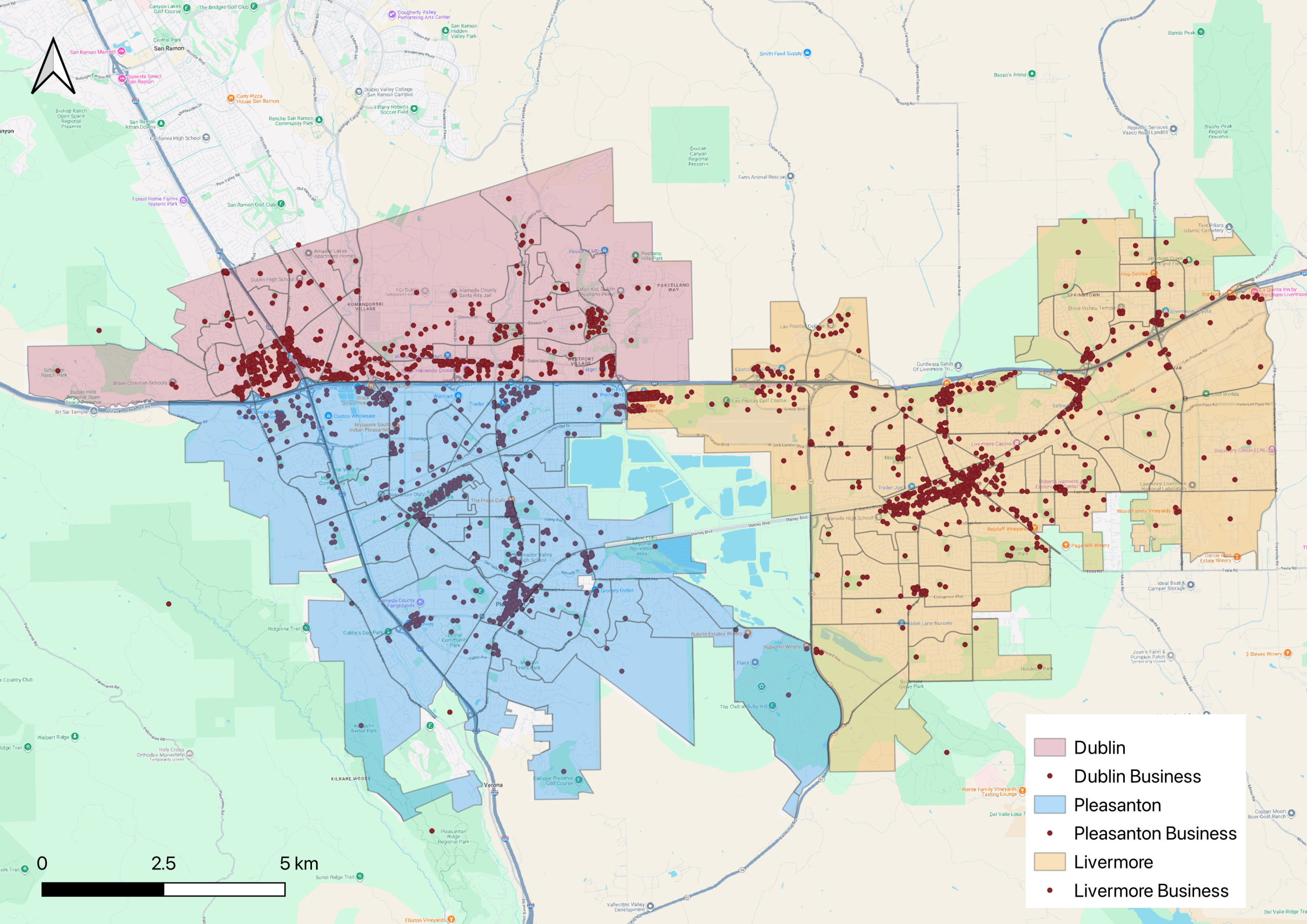
This study focused on three neighboring cities in Alameda County, California: Dublin, Pleasanton, and Livermore. These cities shared the same local economy and transportation network. However, each city had different patterns. Dublin had newer and more mixed-use areas, Pleasanton had a well-established downtown, and Livermore had a lower density environment. These differences were relevant to the cities’ land use and business patterns.

City or County	Land Area (Acres)	Census Block Groups	Population	Dominant Land Use Pattern
Dublin	9747.2	24	72589	Mixed use growth
Pleasanton	15552.0	59	79871	Established downtown
Livermore	16921.6	60	87955	Low density, dispersed
Alameda County	~472000.0	1134	1649060	Mixed urban, suburban, agricultural, and open space

Data Sources

This study used multiple publicly available datasets, including American Community Survey demographic data³, official city boundary files²¹, census block group boundaries²², city parcel⁴and assessor use code records⁵, business and point-of-interest (POI) data²³, and street network data²⁴, to study business type distribution at the neighborhood level. Business POI data were obtained from OpenStreetMap²⁵ using the OSMnx Python library²⁴. Parcel and use code information defined where different business types were legally permitted. Data were aligned to the same census block group so they could be used for feature engineering and machine learning analysis²².

American Community Survey demographic data were obtained from the U.S. Census Bureau American Community Survey (ACS) 5-year estimates, which provided socioeconomic information³. The ACS tables used in this study included B01003 (Total Population), which measured population size; B01001 (Sex by Age), which reflected age and sex distribution; B03002 (Hispanic or Latino Origin by Race), which described race and Hispanic or Latino origin; B15003 (Educational Attainment for the Population 25 Years and Over), which indicated education levels; B19013 (Median Household Income in the Past 12 Months), which measured household income; B25044 (Tenure by Vehicles Available), which measured vehicle availability by housing tenure; B25003 (Tenure), which described owner and renter occupancy; B25002 (Occupancy Status), which indicated vacancy patterns; and B25064 (Median Gross Rent (Dollars)), which measured rental housing cost.

Feature Engineering

Feature engineering turned raw data into model input variables for machine learning. In this study, spatial data, demographic data, and business data were converted into features for each zone. These features included population demand, business supply, land use, distance to major roads and selected infrastructure, and zone rules. The training dataset included all Alameda County 1,134 census block groups, treated as analysis zones, while Dublin, Pleasanton, and Livermore were used as the main case study cities for spatial interpretation and mapping.

Feature Construction

Demographic features were constructed by attaching American Community Survey (ACS) data to each zone³. A summary of the extracted ACS source fields, corresponding model features, and their relevance to model feature construction was provided in Table 2.

ACS Table	Extracted ACS Fields	Model Feature Name	Business Relevance
B01003 – Total Population	B01003_001E	pop_total	Population size
B03002 – Hispanic or Latino Origin by Race (Race / Ethnicity)	B03002_001E	pop_race_total	Race and Hispanic or Latino origin
	B03002_003E	race_white
	B03002_006E	race_asian
	B03002_012E	race_hispanic
B01001 – Sex by Age (Age Structure)	B01001_001E	age_sex_age_total	Age based patterns
	B01001_003E + B01001_027E	age_under5_total
	B01001_006E + B01001_030E	age_15_17_total
	B01001_010E + B01001_034E	age_22_24_total
	B01001_013E + B01001_037E	age_35_39_total
	B01001_017E + B01001_041E	age_55_59_total
	B01001_025E + B01001_049E	age_85plus_total
B15003 – Educational Attainment for the Population 25 Years and Over (Education)	B15003_001E	edu_total_25plus	Education level
	B15003_017E	edu_high_school_grad
	B15003_022E	edu_bachelors
	B15003_023E	edu_masters
B19013 – Median Household Income in Past 12 months (Income)	B19013_001E	median_household_income	Household income
B25003 – Tenure (Housing Tenure)	B25003_002E	tenure_owner_occupied	Residential stability
B25002 – Occupancy Status (Housing Vacancy)	B25002_003E	occupancy_vacant_housing	Vacancy pattern
B25064 – Median Gross Rent (Housing Cost)	B25064_001E	median_gross_rent	Rental housing cost
B25044 – Tenure by Vehicles available (Vehicle Access)	B25044_001E	hh_vehicles_total	Vehicle availability
	B25044_003E + B25044_010E	veh_0
	B25044_004E + B25044_011E	veh_1

Business location features were constructed by measuring existing businesses within each zone. OSMnx²⁴ was used to query and download business POIs associated with commercial and service tags. Restaurant and supermarket locations were extracted from OpenStreetMap²³ using predefined key value tag pairs. The restaurant category included amenity=restaurant, amenity=pub, amenity=bar, and amenity=food_court. The supermarket category included shop=supermarket, shop=grocery, shop=general, shop=health_food, and shop=dairy. Duplicate records with the same business name and location were removed. Because business closure status was not consistently available for all OpenStreetMap²⁵ records, a sensitivity analysis was used to assess inactive business label noise. Lifecycle and closure indicators, including inactive, closed, construction, and end date related fields, were preserved when available. Sensitivity results showed that none of the 234 supermarkets had a closure indicator, while 8 out of 2,292 restaurants had a closure indicator. Inactive POIs were filtered out, and the remaining POIs were joined to the census block group zones²² for feature construction and model training. For restaurants and supermarkets, two features were created: the total number of businesses in each zone, and business density per 100 residents.

Accessibility features were used to measure proximity to key services. Distance based features were computed from each zone’s centroid to the nearest major road, the nearest Bay Area Rapid Transit (BART) station, and the nearest large retail center. Locations of parks, schools, and libraries were also collected as POIs and used to calculate additional distance features^25,24. Euclidean distances provided a consistent proximity measure from each zone center to nearby roads, infrastructure, and POIs. These distances were approximate and did not represent street network travel distance. In addition, intersection density was calculated as a measure of local street connectivity. 

Parcel based features were also created to represent areas available for commercial use. Zoning constraints were converted into binary indicators using parcel use code values^4,5. For each zone and business type, such as restaurants or supermarkets, zoning_allows_<type> was set to 1 if any parcel in the zone had a use code that allowed that business type, and 0 otherwise.

Label Definition and Sensitivity Test

Separate limited service labels were created for restaurants and supermarkets. These labels were used as the target labels for the machine learning models. A zone was labeled as limited service for restaurants or supermarkets when the selected category was allowed by zoning, no business in that category was located inside the zone, and the number of nearby businesses in that category met the threshold tested in the sensitivity analysis.

A sensitivity test compared 300 m and 500 m buffer distances and tested whether the nearby business threshold should be 0 or 1 (Table 3). The final rule selected a 300 m buffer distance and a threshold of 0 nearby businesses, which gave a relatively clear and conservative definition of limited service without making the label too broad (Supermarket 45.0% labeled limited service in Livermore) or too rare (Restaurant 1.7% labeled limited service in Pleasanton) for the three study cities. In this study, a limited service zone was defined as an area where the selected business type, restaurant or supermarket, was allowed, and no business of that type was located either inside the zone or within the surrounding 300 m area.

Buffer (m)	Thres- hold	Type	County (%)	Dublin (%)	Pleasanton (%)	Livermore (%)
300	0	Supermarket	318 (28.0%)	4 (16.7%)	7 (11.9%)	20 (33.3%)
300	0	Restaurant	95 (8.4%)	2 (8.3%)	3 (5.1%)	5 (8.3%)
300	1	Supermarket	503 (44.4%)	7 (29.2%)	15 (25.4%)	27 (45.0%)
300	1	Restaurant	159 (14.0%)	2 (8.3%)	3 (5.1%)	5 (8.3%)
500	0	Supermarket	215 (19.0%)	2 (8.3%)	5 (8.5%)	17 (28.3%)
500	0	Restaurant	50 (4.4%)	2 (8.3%)	1 (1.7%)	3 (5.0%)
500	1	Supermarket	386 (34.0%)	4 (16.7%)	12 (20.3%)	25 (41.7%)
500	1	Restaurant	104 (9.2%)	2 (8.3%)	1 (1.7%)	4 (6.7%)

A small set of derived features was also added to improve model learning which are summarized in Table 4.

Derived Feature	Calculation Method	Purpose
ratio_large_retail_to_major_road	Distance to large retail ÷ distance to major road	Captures balance between commercial access and road access
log_income	Natural logarithm of median household income	Helps balance uneven income values
norm_dist_major_road	Distance to major road normalized to [0,1]	Standardizes road accessibility
norm_dist_bart_station	Distance to nearest BART station normalized	Standardizes transit accessibility
norm_dist_large_retail	Distance to nearest large retail center normalized	Standardizes access to retail
norm_dist_park	Distance to nearest park normalized	Standardizes access to amenities
norm_dist_school	Distance to nearest school normalized	Standardizes how close an area is to schools
norm_dist_library	Distance to nearest library normalized	Represents access to public facilities

Feature Cleaning and Model Input Preparation

Feature preparation was conducted for all Alameda County zones. Although the maps focused on Dublin, Pleasanton, and Livermore, the machine learning dataset was built from the countywide set of zones to provide a larger and more varied modeling dataset. For restaurants and supermarkets, the processed features and limited service labels were converted into final model input tables by constructing a feature matrix X and target labels y. Zone IDs were kept with the tables to make sure that features, labels, and later map outputs matched the correct zones.

After the features and target labels were created, the dataset was cleaned before model training. ID fields, geometry fields, text fields, and target related columns were removed from the predictor feature matrix. To reduce target leakage, business supply variables related to the target label creation were also removed. These included the total number of businesses in each zone, business density per 100 residents, and binary zoning allowance indicators zoning_allows_<type>. For the remaining numeric features, missing values were filled using column means. After missing values were handled, all numeric predictor features were standardized using scikit-learn’s StandardScaler before model training²⁶.

Machine Learning Models

The study tested three models to predict restaurant and supermarket limited service zones. Logistic Regression was selected as a baseline because it was suitable for smaller datasets, while Random Forest and Gradient Boosting models were used because they could capture nonlinear relationships among predictor features. For restaurants and supermarkets, all models were trained and evaluated separately. The cleaned feature matrices from the Feature Cleaning and Model Input Preparation step were used as input for all candidate models.

Model Training and Hyperparameter Tuning

Model performance was evaluated using stratified five fold cross-validation with all Alameda County zones²⁶. This divided the dataset into five folds while keeping similar proportions of limited service and non limited service zones in each fold. Logistic Regression was used as a baseline model, while Random Forest and Gradient Boosting were tested with hyperparameter tuning. Logistic Regression used class_weight=”balanced”, max_iter=1000, random_state=42, scikit-learn’s default lbfgs solver and L2 regularization. Hyperparameter tuning for Random Forest and Gradient Boosting was conducted with RandomizedSearchCV, using F1 score as the main scoring metric and a fixed random seed of 42 for reproducibility. Random Forest was tuned with 50 random search iterations, while Gradient Boosting was tuned with 30 iterations. Because limited service and non limited service zones were not evenly balanced, class imbalance was handled using model weights during training. Logistic Regression and Random Forest used class_weight=”balanced”, while Gradient Boosting used sample weights calculated with scikit-learn’s compute_sample_weight(class_weight=”balanced”, y=y)²⁶. The final cross-validation results were reported using standard metrics: accuracy, precision, recall, and F1 score²⁷. The F1 score was the main evaluation metric because it balanced precision and recall and is suitable for uneven target labels. For each business type, restaurant or supermarket, the model with the highest F1 score was chosen as the final model and saved for final prediction and mapping.

Out-of-fold Prediction for Error Analysis

After the best model was selected for restaurants and supermarkets, out-of-fold prediction was used with stratified five fold cross-validation²⁶. In this step, a new copy of the selected model with the same hyperparameters was created in each fold. The newly created model was then trained on four folds and used to predict the held out fold, so each zone was predicted by a model that had not been trained on that zone. This produced out-of-fold predicted labels and probabilities for each zone. These results were used in the Error Analysis Results section to show whether each predicted label matched the calculated limited service label.

Model Interpretation and Prediction

After selecting the best model, feature importance was analyzed to identify variables that contributed most to predictions. The importance of each variable was calculated based on the model type, and variables were ranked from most important to least important. The selected models for restaurants and supermarkets were then used to generate limited service zone predictions and probabilities. Model outputs were used directly for mapping and result analysis.

Results

Model Selection and Tuned Hyperparameter Results

Model performance was compared separately for restaurants and supermarkets using stratified five fold cross-validation. Cross-validation accuracy measured how often a model correctly classified data. The cross-validation F1 score, which was the harmonic mean of precision and recall, was used as the primary metric to balance precision and recall for uneven target labels²⁷. Cross-validation ROC-AUC measured a model’s ability to distinguish limited service and non limited service zones and was also used to evaluate performance. Based on cross-validation results, Random Forest was selected as the best model for supermarkets, and Gradient Boosting was selected as the best model for restaurants. These results suggested that restaurant and supermarket limited service patterns were related to the predictor features in different ways. The highest performing models across the candidate models were provided in Table 5.

Business Type	Model	Accuracy	F1	ROC AUC
Restaurant	Gradient Boosting	0.887	0.315	0.780
Supermarket	Random Forest	0.638	0.518	0.723

The final model hyperparameters were reported in Table 6. Random Forest and Gradient Boosting were tuned using RandomizedSearchCV, with F1 score as the main scoring metric. The selected hyperparameters were used in the final models for prediction and interpretation.

Business type	Final model	Tuning method	Final parameter settings
Restaurant	Gradient Boosting	RandomizedSearchCV	n_estimators=200, learning_rate=0.05, max_depth=3, min_samples_split=2, min_samples_leaf=1, subsample=1.0,  random_state=42
Supermarket	Random Forest	RandomizedSearchCV	n_estimators=200, max_depth=5, min_samples_split=5, min_samples_leaf=4, max_features=”sqrt”, random_state=42

Spatial Patterns and Feature Importance Results

Figure 2 and Figure 3 showed the distribution of calculated and predicted limited service zones for restaurants and supermarkets in the three study cities. Supermarket limited service zones were more widespread than restaurant limited service zones. Restaurant limited service zones tended to occur away from major commercial areas and city centers. The predicted zones generally followed the calculated zones, although the model predicted additional limited service zones in all three cities. Few calculated limited service zones were missed by the model. Among the three cities, Livermore had the highest number of restaurant and supermarket limited service zones, and these zones were distributed across a larger part of the city.

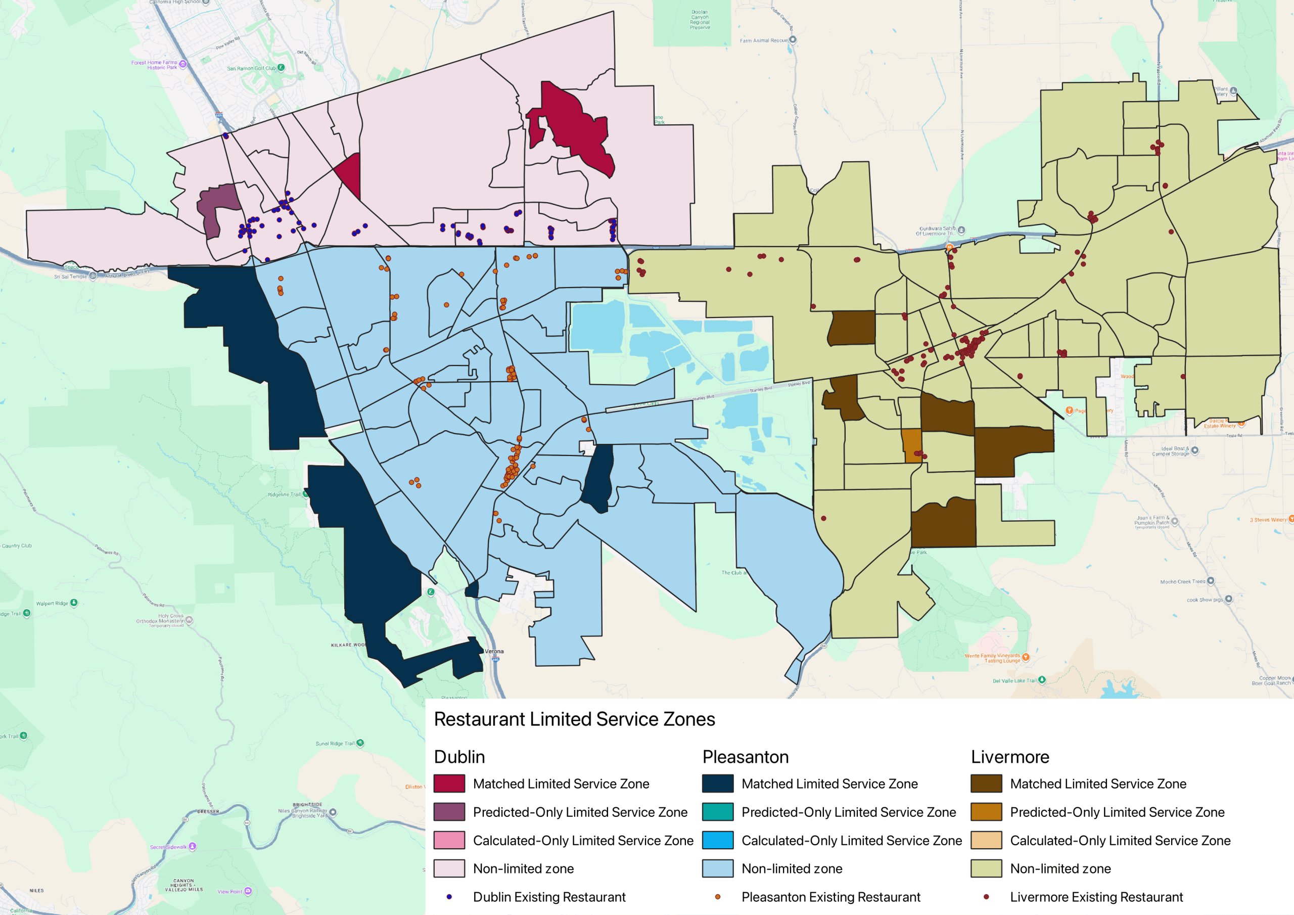
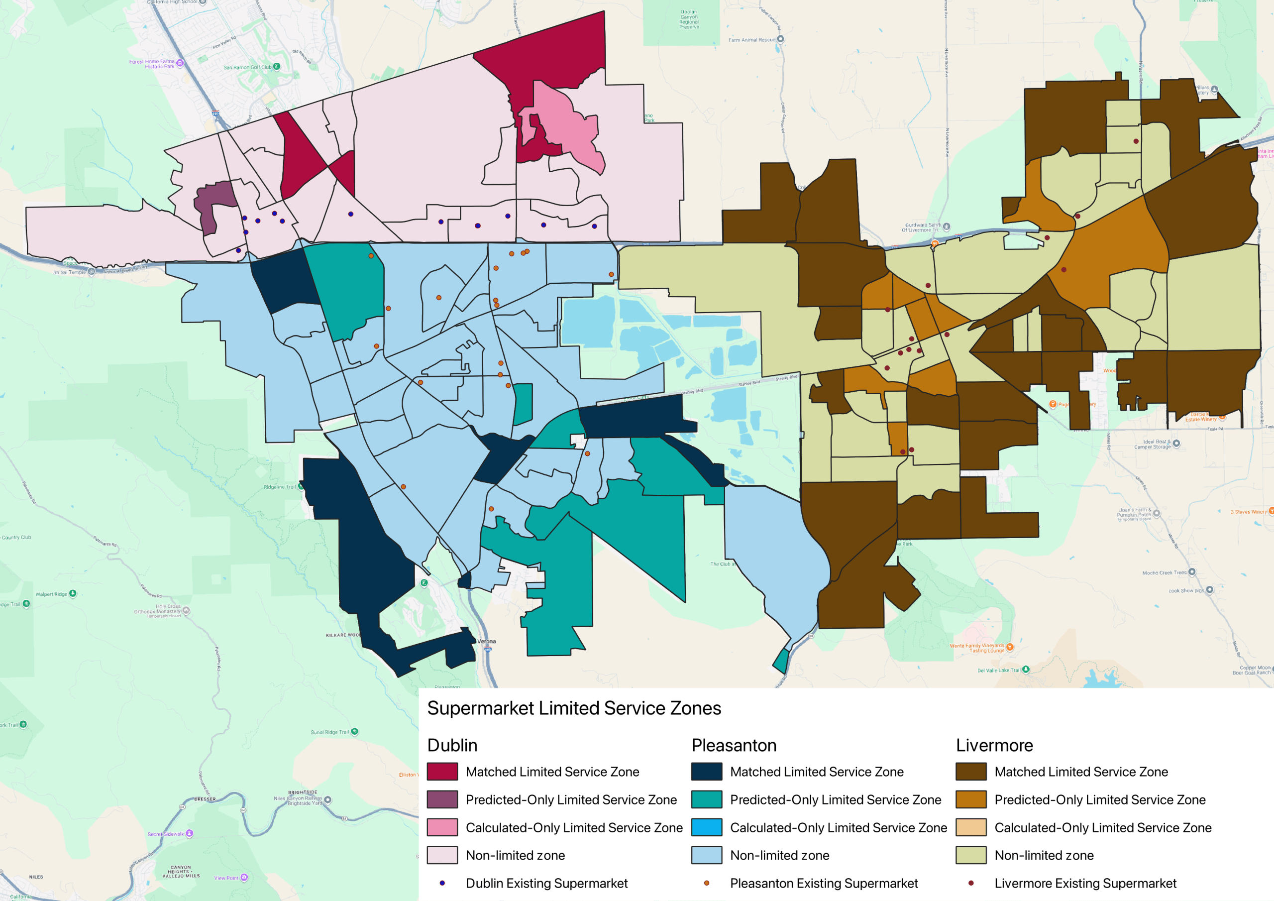
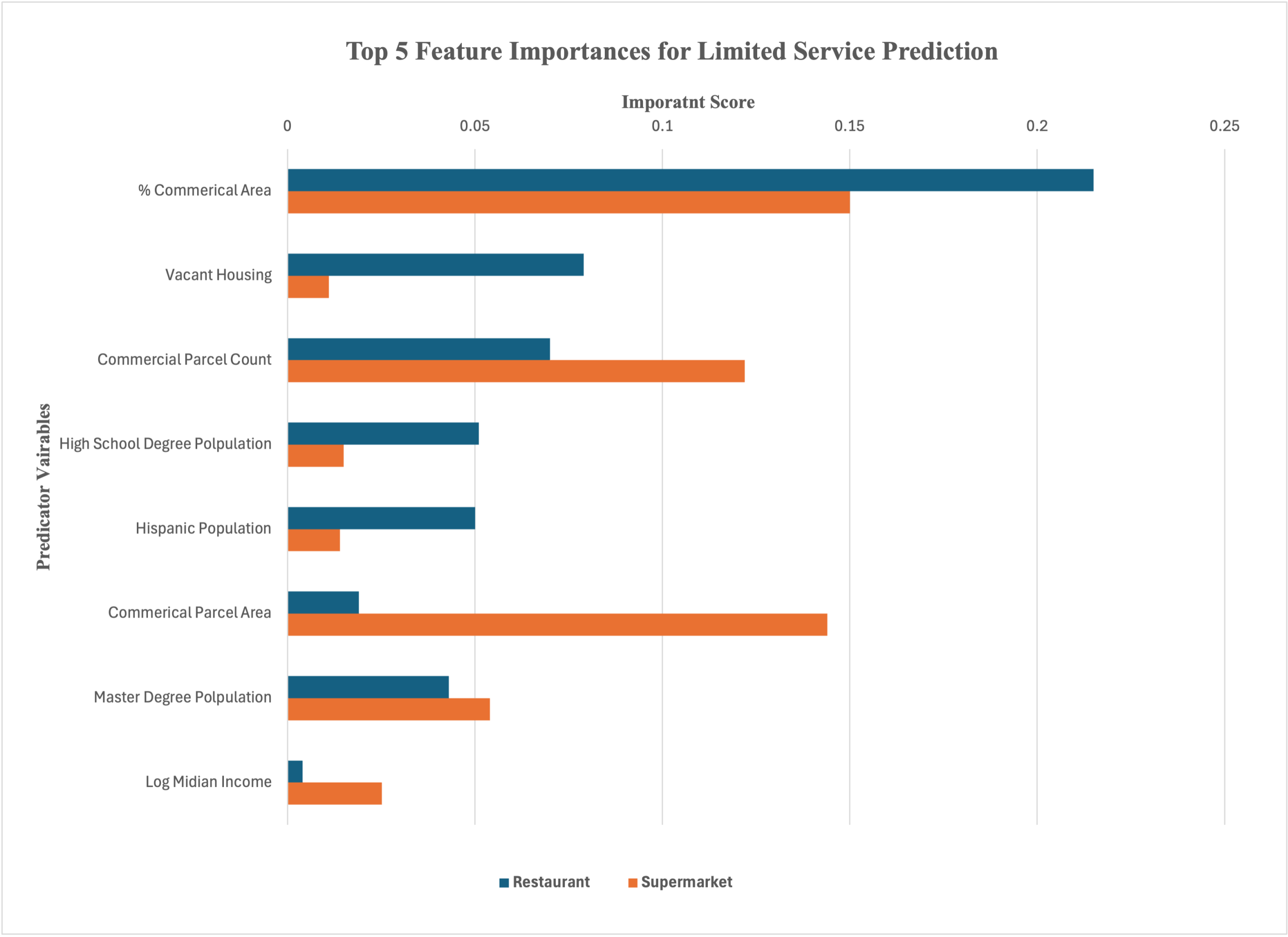
Figure 4 showed the feature importance results for the selected restaurant and supermarket prediction models. For restaurants, the model included 44 features, with importance scores ranging from 0.000 to 0.215. The five highest ranked features were % Commercial Area (0.215), Vacant Housing (0.079), Commercial Parcel Count (0.070), High School Degree Population (0.051), and Hispanic Population (0.050). The highest ranking restaurant feature was % Commercial Area, which measured the share of parcel area that was commercial. For supermarkets, the model included 44 features, with importance scores ranging from 0.005 to 0.150. The five highest ranked features were % Commercial Area (0.150), Commercial Parcel Area (0.144), Commercial Parcel Count (0.122), Master’s Degree Population (0.054), and Log Median Income (0.025). Overall, commercial land use and parcel features ranked highly for both business types, followed by selected demographic variables.

Out-of-Fold Prediction Error Analysis Results

After the best model was selected for restaurants and supermarkets, out-of-fold prediction was used to examine incorrect predictions and perform error analysis. The out-of-fold error analysis was based on all 1,134 Alameda County zones. This differed from the map interpretation, which focused on Dublin, Pleasanton, and Livermore, because model validation was based on the full countywide modeling dataset.

Business type	Model	True positive	False positive	False negative	True negative	Matched	Mismatched
Restaurant	Gradient Boosting	29	62	66	977	1006	128
Supermarket	Random Forest	218	281	100	535	753	381

Business type	Matched zones (%)	Mismatched zones (%)	False positive (%)	False negative (%)
Restaurant	88.71%	11.29%	5.47%	5.82%
Supermarket	66.40%	33.60%	24.78%	8.82%

The confusion matrix and error percentage results showed more matched predictions for the restaurant model than the supermarket model across Alameda County. The restaurant model matched 1,006 of 1,134 zones and had 128 mismatched zones, while the supermarket model matched 753 of 1,134 zones and had 381 mismatched zones. For restaurants, false positives and false negatives were nearly equal, with 62 false positives and 66 false negatives. For supermarkets, there were more false positives, with 281 false positives compared with 100 false negatives.

Discussion

Model Performance and Error Patterns

The results showed that machine learning models could help identify limited service zones, although performance differed between restaurants and supermarkets. In the model evaluation results, Gradient Boosting performed best for restaurants, and Random Forest performed best for supermarkets. This difference may be related to how restaurants and supermarkets are distributed across the study area, but model results alone cannot confirm this explanation. For restaurants with highly unbalanced target labels (8.4% positive), Gradient Boosting had high accuracy (0.887) and ROC AUC (0.780), although the F1 score was much lower (0.315). The low F1 score indicates that the restaurant model correctly predicted many zones without limited service, but was less consistent at predicting the smaller group of limited service zones. For supermarkets with less uneven target labels (28.0% positive), Random Forest had lower accuracy (0.638) and a higher F1 score (0.518), indicating that it performed better at identifying limited service zones while reducing incorrect predictions. This contrast also shows that F1 is a better selection metric for this dataset than accuracy.

The out-of-fold error analysis showed that the restaurant model (88.71% matched zones) had more matched predictions than the supermarket model (66.40% matched zones). The restaurant errors were relatively balanced, with 5.47% false positives and 5.82% false negatives. The supermarket model had 24.78% false positives compared with 8.82% false negatives, suggesting that the model more often classified a zone as limited service when the calculated label did not. This pattern may be related to the fact that existing supermarkets are fewer and more unevenly distributed than restaurants, making their limited service patterns harder to predict. The higher number of supermarket false positives may also be related to the use of class_weight=”balanced” in the Random Forest model, which gives more weight to the smaller group of limited service zones and may increase the number of zones predicted as limited service.

Spatial Patterns and Important Local Factors

The prediction maps showed that limited service zones were not evenly distributed across the study area. Supermarket limited service zones were more widespread, while restaurant limited service zones were fewer. This difference could be related to how the business types operate. Restaurants are more common and can be located in smaller commercial areas, while supermarkets are less common and serve larger areas, so more zones may lack a nearby supermarket. The predicted zones generally followed the calculated limited service zones, which indicates that the models identified the main areas where limited service zones appeared. However, the models also predicted additional limited service zones in all three cities. Among the three cities, Livermore had the most limited service zones for both restaurants and supermarkets, and these zones were distributed across more areas of the city. This may be related to Livermore’s larger area and lower density environment compared with Dublin and Pleasanton. 

The feature importance results showed that commercial land features ranked highly for both restaurant and supermarket models. For restaurants, % Commercial Area had the highest importance score, followed by Vacant Housing and Commercial Parcel Count. For supermarkets, the most important features were also related to commercial land use, including % Commercial Area, Commercial Parcel Area, and Commercial Parcel Count. This suggests that limited service zones were connected to whether an area had commercial space and commercial parcels available. Demographic features also ranked among the top five features, but their importance scores were lower than the highest ranked commercial features. The results suggest that limited service patterns were most closely associated with commercial land availability, while demographic and housing variables contributed less to model prediction.

Limitations

This study has several limitations that should be considered when interpreting the results. Business location data come from open source sources, where some businesses may be missing or misclassified. This issue may affect estimates of business supply in some zones. Demographic data come from the American Community Survey, which is based on sample estimates. As a result, values at the census block group level may include sampling error that affects the precision of the analysis. Census block groups are used to divide the area into smaller zones, although they may not fully reflect residents’ access to nearby services. Limited service labels are defined as a zone where the selected business type is allowed, and no business of that type is located either inside the zone or within the surrounding 300 m area, rather than a universal service standard. 

The dataset size is also limited because the number of census block groups within the county is relatively small. Because each model was trained on only 1,134 zones, the limited training data may affect model stability and reduce the generalizability of the findings to other urban areas. Cross-validation and out-of-fold prediction help reduce this risk, but they do not remove it completely. 

Another limitation is the possible risk of data leakage and overfitting. Because the limited service label was created from business location information, predictor variables that are closely related to the target label could cause the model to learn patterns tied to the label definition. To reduce this problem, business supply variables, such as business count, business density, and zoning allowance features, were removed from the model input. Some remaining features may still be indirectly related to where businesses are located, so the model may partially learn these patterns. Overfitting is also a possible limitation because the models were trained and evaluated on the same countywide study region. Results may not apply directly to areas with different urban settings or populations. Therefore, this case study should be viewed as one example of how machine learning can support the identification of possible local limited service areas.

Finally, feature importance identifies which variables had the highest importance in model prediction but cannot prove those variables cause limited service. Results may also vary depending on model settings and the chosen algorithm.

Conclusion

This study explored whether GIS-based features and machine learning models could identify possible local limited service zones for restaurants and supermarkets. The results showed that limited service patterns differed by business type, with supermarket limited service zones appearing more widespread than restaurant limited service zones. The selected model also differed by business type, with Gradient Boosting selected for restaurants and Random Forest selected for supermarkets. The restaurant model had a lower F1 score than the supermarket model, indicating that the restaurant model identified limited service zones less consistently. The prediction maps showed that predicted limited service zones generally followed the calculated limited service zones, although the models also predicted some additional limited service zones. The feature importance results showed that commercial land use features were key predictors for both business types. This study should be viewed as an example of how GIS and machine learning can support the identification of possible local limited service zones. The results should be interpreted as predictions and not confirmed proof of limited service.

Several limitations should be considered when interpreting these findings. The dataset is limited and relies on open source business location data and demographic estimates based on American Community Survey data. Survey data may include missing entries or sampling error.  Because the limited service label was created from business location data, there is a possible risk of data leakage, even after business count, business density, and zoning allowance features were removed. Some remaining features may still give the model clues about where businesses are located. Furthermore, overfitting is possible because the models were trained and tested within a small countywide study area, which may limit the generalizability of the results. In addition, machine learning models can identify relationships within the data, but they cannot prove these relationships cause limited service. 

Future work could improve the study by defining limited service zones with more independent data, removing features that are directly tied to the label, carefully checking variables that may be indirectly related, and testing the models on a separate geographic area. Future work could also compare results across more cities, use street network accessibility instead of centroid based Euclidean distance, and include additional local factors such as rent, transportation access, business competition, and consumer demand. With these improvements, future research could produce more reliable model results and provide stronger evidence for identifying areas that may need closer review.

References

1. N. Mahmud, M. A. Habib. A comprehensive business location choice model leveraging machine learning in systematic choice set. Transportation Research Record. Vol. 2678, pg. 1856-1871, 2024, https://doi.org/10.1177/03611981241253609. [↩] [↩]
2. L. Herbert, D. P. Giovenco, I. Flores, M. Chen, B. C. Lowery, E. Chery-Mullen, M. Meaney, A. Y. Kong. Patterns of tobacco retailer counts by zoning designations and sociodemographic characteristics in Oklahoma City and Tulsa, Oklahoma. Health & Place. Vol. 95, pg. 103496, 2025, https://doi.org/10.1016/j.healthplace.2025.103496. [↩]
3. U.S. Census Bureau. American community survey (ACS) 5-year estimates. https://data.census.gov, Accessed 2026. [↩] [↩] [↩] [↩]
4. Alameda County ALCO Data Portal. Parcels. https://data.acgov.org/datasets/2b026350b5dd40b18ed7a321fdcdba81_0/explore, Accessed 2026. [↩] [↩] [↩]
5. Alameda County ALCO Data Portal. Assessor Office Use Codes. https://data.acgov.org/datasets/7711de7634e24cf19979daba73561691_0/explore, Accessed 2026. [↩] [↩] [↩]
6. T. P. Broadbridge, J. E. F. Green, S. P. Preston, N. T. Fadai, J. Maclean. Food purchase data reveals the locations of London’s ‘food deserts’. PLOS Complex Systems. Vol. 2, pg. e0000072, 2025, https://doi.org/10.1371/journal.pcsy.0000072. [↩] [↩]
7. C. Tudor. A geospatial framework for retail suitability modelling and opportunity identification in Germany. ISPRS International Journal of Geo-Information. Vol. 14, pg. 342, 2025, https://doi.org/10.3390/ijgi14090342. [↩] [↩] [↩]
8. V. Chaturvedi, W. T. de Vries. Machine learning algorithms for urban land use planning: A review. Urban Science. Vol. 5, pg. 68, 2021, https://doi.org/10.3390/urbansci5030068. [↩] [↩] [↩]
9. L. Sun, W. Liu, Q. Liu. Decoding green space supply-demand mismatch through urban morphology: toward equitable urban planning with explainable machine learning. PLOS ONE. Vol. 21, pg. e0342596, 2026, https://doi.org/10.1371/journal.pone.0342596. [↩] [↩] [↩]
10. S. Dreiseitl, L. Ohno-Machado. Logistic regression and artificial neural network classification models: a methodology review. Journal of Biomedical Informatics. Vol. 35, pg. 352-359, 2002,  https://www.sciencedirect.com/science/article/pii/S1532046403000340. [↩]
11. L. Breiman. Random Forests. Machine Learning. Vol. 45, pg. 5-32, 2001, https://link.springer.com/article/10.1023/A:1010933404324. [↩]
12. J. H. Friedman. Greedy function approximation: a gradient boosting machine. The Annals of Statistics. Vol. 29, pg. 1189-1232, 2001, https://doi.org/10.1214/aos/1013203451. [↩]
13. C. A. Hidalgo, E. Castañer, A. Sevtsuk. The amenity mix of urban neighborhoods. Habitat International. Vol. 106, pg. 102205, 2020, https://doi.org/10.1016/j.habitatint.2020.102205. [↩]
14. A. Sevtsuk. Location and agglomeration: the distribution of retail and food businesses in dense urban environments. Journal of Planning Education and Research. Vol. 34, pg. 374-393, 2014, https://doi.org/10.1177/0739456X14550401. [↩]
15. S. Wu, B. Chen, J. An, A. Nelson, F. Dai, C. Lin, P. Gong. Measuring global human accessibility to essential daily necessities and services. Nature Communications. Vol. 16, pg. 10709, 2025, https://doi.org/10.1038/s41467-025-65732-w. [↩]
16. D. Yang, J. Zhao, P. Xu. Deep learning-based approach for optimizing urban commercial space expansion using artificial neural networks. Applied Sciences. Vol. 14, pg. 3845, 2024, https://doi.org/10.3390/app14093845. [↩]
17. J. Zhang, J. Song, J. Zeng. Toward resilience: assessing retail location’s complex impact mechanism using PLS-SEM aided by machine learning. Sustainability. Vol. 17, pg. 7461, 2025, https://doi.org/10.3390/su17167461. [↩]
18. Y. Zheng, Y. Lin, L. Zhao, T. Wu, D. Jin, Y. Li. Spatial planning of urban communities via deep reinforcement learning. Nature Computational Science. Vol. 3, pg. 748-762, 2023, https://doi.org/10.1038/s43588-023-00503-5. [↩]
19. Y. Hu, K. Qin, S. Wang. GeoPPO—a location-allocation method of superstores based on deep reinforcement learning—a case study of Xi’an. ISPRS International Journal of Geo-Information. Vol. 15, pg. 114, 2026, https://doi.org/10.3390/ijgi15030114. [↩]
20. Y. Yue, G. Yan, T. Lan, R. Cao, Q. Gao, W. Gao, B. Huang, G. Huang, Z. Huang, Z. Kan, X. Li, D. Liu, X. Liu, D. Ma, L. Wang, J. Xia, X. Yang, M. Zhou, A. G.-O. Yeh, R. Guo, C. Claramunt. Shaping future sustainable cities with AI-powered urban informatics: Toward human-AI symbiosis. Computational Urban Science. Vol. 5, pg. 31, 2025, https://doi.org/10.1007/s43762-025-00190-0. [↩]
21. Alameda County ALCO Data Portal. Cities. https://data.acgov.org/datasets/d9c9fd5822aa41ca90867845c58df6aa_0/explore, Accessed 2026. [↩]
22. U.S. Census Bureau. TIGER/Line shapefile, current, state, California, block group. https://catalog.data.gov/dataset/tiger-line-shapefile-current-state-california-block-group, Accessed 2026. [↩] [↩] [↩]
23. OpenStreetMap contributors. OpenStreetMap database. https://www.openstreetmap.org, Accessed 2026. [↩] [↩]
24. G. Boeing. OSMnx: new methods for acquiring, constructing, analyzing, and visualizing complex street networks. Computers, Environment and Urban Systems. Vol. 65, pg. 126-139, 2017, https://doi.org/10.1016/j.compenvurbsys.2017.05.004. [↩] [↩] [↩] [↩]
25. OpenStreetMap contributors. OpenStreetMap database. https://www.openstreetmap.org, Accessed 2026. [↩] [↩] [↩]
26. F. Pedregosa, G. Varoquaux, A. Gramfort, V. Michel, B. Thirion, O. Grisel, M. Blondel, P. Prettenhofer, R. Weiss, V. Dubourg, J. Vanderplas, A. Passos, D. Cournapeau, M. Brucher, M. Perrot, E. Duchesnay. Scikit-learn: machine learning in Python. Journal of Machine Learning Research. Vol. 12, pg. 1856-1871 and pg. 2825-2830, 2011, https://jmlr.org/papers/v12/pedregosa11a.html. [↩] [↩] [↩] [↩]
27. D. M. Powers. Evaluation: from precision, recall and F-measure to ROC, informedness, markedness & correlation. Journal of Machine Learning Technologies. Vol. 2, pg. 37-63, 2011, https://bioinfopublication.org/files/articles/2_1_1_JMLT.pdf. [↩] [↩]