Price Prediction From Auction Log Data

Abstract

The auctioning of Cartier wristwatches, Palm Pilot M515 PDAs, and Xbox game consoles has faced ongoing difficulties in mitigating deceptive practices, and often prompts bidders to overspend due to emotional attachment to items. Predicting auction end prices could help auctioneers optimize settings for greater profit, reduce deception by accurately representing item values, and promote fairer, more balanced transactions. In this study, we develop a regression model to predict the end price of an auction using historical auction data for three eBay product categories. Using Jank and Shmueli’s eBay Auction Results Dataset, we tested Ridge, XGBoost, Random Forest Regressor, Linear Regression, and MLPRegressor, and quantified error margins using mean absolute error (MAE) and root mean squared error (RMSE) determine the model that best predicts the end price. MAE is the average absolute difference between predicted and actual prices, while RMSE is the square root of the average of the squared differences between the predicted and actual prices. The Ridge and Linear Regression models bested other models, both making mean absolute error predictions of about $18 (±$4). The accurate results of these models can predict if sellers are making a fair profit on an auction and inform auctioneers about final price information, cautioning against overspending. Our models also supply another aspect of AI modeling for auction predictions, creating more accurate baseline models for the entire industry to use. For sellers seeking quick profit, a 3-day auction is more logical than a 5-day auction, as extending the auction duration from three to five days does not increase profit. While 7-day auctions yield higher selling prices overall, 3-day and 5-day auctions achieve similar results; therefore, a 3-day auction offers the fastest return.

Keywords: error metrics, k-fold cross validation, neural network, train-test split, regression, decision trees

Introduction

The industry of auctioning is a field of economic advantages, with various auctioning strategies emerging across the field in order to strategically mold auctions to the auctioneer’s liking. Overall, auctions have been considered to be fairly unpredictable because of human behavior and the large variance of bidding backgrounds, creating a challenging problem of auction end price prediction^1,2,3. Dan Ariely, Axel Ockenfels, and Alvin E. Roth found that hard deadlines on auctions cause individuals to snipe bids, placing higher bids during the last seconds in an effort to win, while also greatly altering final prices^4,5,6. As described in Stephanie Lotz’s doctoral dissertation “Emotions in auctions: When and why bidders overbid”, individuals often become invested in the auction and overbid when feeling extreme winner and loser emotions, meaning it is extremely difficult to predict bidder behavior precisely⁷. Additionally, the internet has enabled global participation in auctions, further complicating predictions and influencing bidder behavior^8,9. The act of predicting auction prices has been extensively studied; many other researchers and innovators have already attempted to solve this challenging problem¹⁰. Li Xuefeng et al.’s work “Predicting the final prices of online auction items” is a notable study in this area. Throughout their article, they mention the “winner’s curse,” where winners of auctions often pay more than the actual price of the item¹¹. AI and end price prediction can help diminish the “winner’s curse” when possible by providing customers with a set price that the auction is estimated to reasonably close at. Additionally, according to “The Winner’s Curse, Reserve, Prices, and Endogenous Entry: Empirical Insights from eBay Auctions” by Patrick Bajari and Ali Hortacsu, the circumstances of many auctions lead to winner’s curse being a constant problem in auctions¹². Anything beyond this price point would mean customers are paying much more than necessary for the auctioned item.

In David Nicholson’s and Rohan Paranjpe’s “A Novel Method for Predicting the End-Price of eBay Auctions,” the authors emphasize the efficiency of the UPNB (Universal Probabilistic Naive Bayes) classifier in predicting the end price¹³. The model’s simplicity and strong performance help it outperform similar models¹³. They found that in the variety of models tested, the simpler model performed the best. Like Nicholson and Paranjpe, we had a similar approach to setting up each AI and using regression for our models; however, we further extended their work to include decision tree regressors with optimized hyperparameters and decision branches. Likewise, we found that simpler regression models, such as Linear Regression and Ridge Regression, achieve similarly strong results. Compared to Nicholson, Paranjpe, Xuefeng, and Lotz, our work tests multiple different models and directly predicts the end prices of auctions, something Xuefeng and Lotz stray from. Using k-fold cross validation, a model evaluation procedure, our work tested five different models from varying machine learning architectures, comparing each to find the best performing predictive model in the tested field using the error metrics of: mean absolute error, root mean squared error, and R² score.

In our central dataset, we studied three different items being sold in online auctions: Cartier Wristwatches, Palm Pilot M515 PDAs, and Xbox game consoles. A limited variety of items being auctioned was the main limitation of our research. This limitation of three different auction items diminish the range of usefulness of the model to other auctions by limiting the adaptability of the models to different auction items, reducing applicability to other auctions. However, it is still highly applicable to those three auction types. We worked to solve the question of: Which model predicts auction end prices best? We applied five different AI models to the auction data which were the Ridge Regressor, MLPRegressor, Linear Regressor, Random Forest Regressor, and XGBoost, in an effort to most accurately predict the end prices of auctions. This paper explains our process including how we modified and calculated new statistical relationships, and trained our five different models to best predict the end prices of auctions. When trained on the statistical data of past auctions on eBay, we hypothesize that Ridge Regression will perform and predict end prices the best.

Methodology

The data we used for these experiments was directly sourced from Wolfgang Jank and Galit Shmueli’s book Modeling Online Auctions, which explains the analysis of online auction data and the applicability of machine learning models to the field, found through this link: https://www.kaggle.com/datasets/onlineauctions/online-auctions-dataset¹⁴. In the dataset we used for our study, there were four main input factors that we focused on in the process of developing an accurate model¹⁵. These were the bid times, opening price, bid amount, and bidder rate.The bidder rate is the eBay feedback rating of the bidder, and scores range from -4 to 3140^16,17. Our target variable was the end price of the auctions. All other features void of statistical values, such as the auction ID and bidder name, were removed from the dataset as they did not contribute to the outcomes of auctions. Additionally, we found that there were 1953 Cartier wristwatch auctions, 5917 Palm Pilot M515 PDA auctions, and 2811 Xbox game console auctions. This means the majority of the data set included Palm Pilot M515 PDA auctions, and could be considered a dominating auction type in our dataset. Our variables were found to be fairly dependent on each other. The bid amounts and bid times depended on previous bids, and the bidder rate depended on how well the bidder performed¹⁸. At the end, the end price depended on all other variables for a set output. This would affect predictions by making it easier for the model to predict the outcome of another model, simply based on the value of another data point.

Name of Variable	Meaning	Units	Input or Target Variable
Bid times	The time in days the bid was placed after the start of the auction	Days	Input
Opening price	The price an auction starts at	Dollars	Input
Bid amount	The amount of money a bidder bids per bid during an auction	Dollars	Input
Bidder rate	eBay feedback rating of the bidder	Feedback rating	Input
End price	The ending price of an auction after all bids are inputted and the auction time has ended	Dollars	Target

Table 1 | Table displaying the variables of the dataset including their definitions, units, and if they are an input or target variable.

Table 1 defines each variable, its unit, and if it is an input or target variable. Before initial model development, we focused on optimizing the dataset through data engineering. First, removing all outliers with an end price over $5000, we prevented any output skewing during model training. We chose to remove the data point above $5000 because of its uniqueness within the data, as there were no other data points above $5000 except that unique auction. There were 11 null values in the bidder rate column and 16 null values in the bidder column, though the bidder column was engineered to be excluded within our data. To fill the 11 null values in the bidder rate column, we averaged the values of the bidder rate column and replaced missing values with the column mean¹⁹. We used the average of the column because of the almost negligible amount of null values in the column, while also training models on numbers that are to an extent common in that row, helping denoise the data. The input of the mean value into null values would barely affect model performance because of the minimal amounts of null values, and would only move model predictions to a more averaged value. We then moved on with data engineering. Understanding that there are possibly more metrics to utilize with the statistics given, we found the standard deviation of various columns while also creating a new column of the averages of the difference in bid times for each auction. After data engineering, we had 10681 instances, with no data samples having raised problems previously.

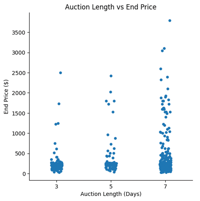
While preparing models, we also began visualizing relationships in the data. An increasingly prominent relationship we found was that the differences in price in a 3-day and 5-day auction are not of significant variance, but instead vary more when compared to a 7-day auction. Observing Figure 1, the difference in end price between a 3-day and 5-day auction is minimal, meaning that if a quick profit is needed, a 3-day auction would not diminish the auctioneer’s expected returns. However, if the auctioneer is fairly patient, they would see an increase in profit: 7-day auctions tend to generate more profit²⁰. With 10681 instances of data, we ran a multivariate regression analysis to evaluate the effect of auction duration on the final price of auctions. In the regression analysis, we controlled item type, opening price, and bidder rating. The results of the regression analysis show that 7-day auctions are associated with significantly higher end prices compared to 3-day auctions (β = 81.84, p = 0.008). Contrastingly, the difference between 3-day and 5-day auctions is not statistically significant (p = 0.361), supporting the idea of 3-day auctions raising about equal prices as 5-day auctions.

These findings are additionally supported by group means, which show overlap in confidence intervals between 3-day and 5-day auctions, but greater separation, and thus, a greater increase in price, for 7-day auctions.

Out-of-sample evaluation yielded an RMSE of 442.97, suggesting moderate predictive performance and supporting the model’s generalizability.

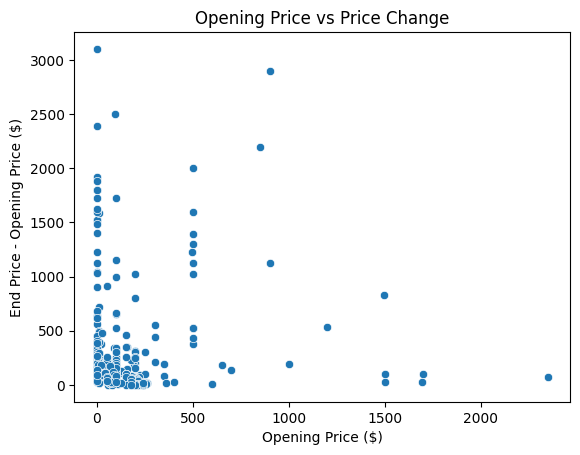
We found that lower opening prices often led to a higher auction final price. Referring to Figure 2, it is seen that the lower the opening price, the higher the difference between opening and ending price of the auction. Though it is not the only factor, it has led us to believe that, even though the opening price sets a minimum standard to the auction, a higher opening price does not incline customers to spend more in an auction.

We fit each of the following AI models onto our dataset and compared how each model reacted using a variety of error metrics. The statistical inputs we utilized consisted of the bid price, bid time, bidder rate, opening price of the auction, end price of an auction, and how long the auction was open for.

All of the models needed hyperparameter tuning except for Linear Regression. This is because Linear Regression simply does not have any tunable hyperparameters to improve performance, including no complexity parameters that control model complexity. Each of the other models have hyperparameters that directly impact model behavior, such as the regularization penalty in Ridge Regression, and the hidden layers hyperparameter in the MLPRegressor. Therefore, we found the hyperparameters for each model that maximized model performance to compare all models in an equal field, where each of them are in their best state. For all the models except Linear Regression, we used GridSearchCV to find the best hyperparameters for each model. The GridSearchCV that was used within the models already incorporated a validation set during training, meaning models were trained on the training set, found best hyperparameters with the validation set incorporated within the GridSearchCV, and tested against the unseen test set of the data. This pipeline creates a clear and organized order of data analysis, and ensures that no data biases are present in the outcomes of model performance. However, RandomSearchCV was used for the MLPRegressor before data engineering because of how resource intensive the MLPRegressor with the GridSearchCV before data engineering was.

Model Name	Search Ranges	Scoring Function	Final Best Hyperparameters	Software Versions	Random Seed
Linear Regression	N/A	N/A	N/A	scikit-learn 1.6.1	N/A
Random Forest Regressor	‘n_estimators’: [100, 200]   ‘max_depth’: [None, 10, 20]   ‘min_samples_split’: [2, 5, 10]   ‘min_samples_leaf’: [1, 2, 4]   ‘max_features’: [‘sqrt’, ‘log2’]	neg_mean_absolute_error	‘max_depth’: 20   ‘max_features’: ‘sqrt’   ‘min_samples_leaf’: 1   ‘min_samples_split’: 2   ‘n_estimators’: 200	scikit-learn 1.6.1	0
Ridge Regression	‘alpha’: [0.001, 0.01, 0.1, 1, 10, 100]   ‘fit_intercept’: [True, False]    ‘solver’: [‘auto’, ‘svd’, ‘cholesky’, ‘lsqr’]	neg_mean_absolute_error	‘alpha’: 100   ‘fit_intercept’: False   ‘solver’: ‘svd’	scikit-learn 1.6.1
MLPRegressor	‘mlp__hidden_layer_sizes’: [         (50,),         (100,),         (50, 50),         (100, 50),         (50, 30, 10)     ],     ‘mlp__activation’: [‘relu’, ‘tanh’],     ‘mlp__alpha’: [0.0001, 0.001, 0.01],     ‘mlp__learning_rate_init’: [0.001, 0.01]	neg_mean_absolute_error	‘mlp__activation’: ‘relu’   ‘mlp__alpha’: 0.0001   ‘mlp__hidden_layer_sizes’: (100, 50)   ‘mlp__learning_rate_init’: 0.01	scikit-learn 1.6.1	1
XGBoost	“n_estimators”: [100, 200]     “max_depth”: [3, 5, 7]     “learning_rate”: [0.01, 0.1, 0.2]     “subsample”: [0.8, 1.0]     “colsample_bytree”: [0.8, 1.0]	neg_mean_absolute_error	‘colsample_bytree’: 0.8   ‘learning_rate’: 0.1   ‘max_depth’: 5   ‘n_estimators’: 200   ‘subsample’: 1.0	scikit-learn 1.6.1	42
Decision Tree Regressor	‘dt__max_depth’: [None, 5, 10, 20, 30]     ‘dt__min_samples_split’: [2, 5, 10, 20]     ‘dt__min_samples_leaf’: [1, 2, 5, 10]     ‘dt__max_features’: [None, ‘sqrt’, ‘log2’]	neg_mean_absolute_error	‘dt__max_depth’: 20  ‘dt__max_features’: None  ‘dt__min_samples_leaf’: 2  ‘dt__min_samples_split’: 2	scikit-learn 1.6.1	1

Linear Regression

A Linear Regression model, mathematically described by the equation:

   

for regression with multiple independent variables, as in our case, is a machine learning algorithm that performs best when predicting a continuous single output from a range of linear input data with outliers modified to be overlooked^21,22. Here β₀ denotes the predicted output of the model, β is the intercept of the model, coefficients β are the weights for each independent variable, the x variables are the independent features, and k is the number of features. As mentioned in Linear and logistic regression models: when to use and how to interpret them? by Horacio Matias Castro and Juliana Carvalho Ferreira, Linear Regression seems to work most efficiently when a variety of independent variables are analyzed by a model to predict on singular continuous output²¹.

Random Forest

The Random Forest Regressor is another machine learning model that was tested on our data, as it divides the dataset into subgroups and utilizes trees to make predictions for each subgroup. The model then averages the outputs of each tree to declare a final prediction, described by:

   

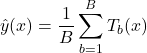
where  is the output, B is the number of trees, b is the tree index, and Tb(x) is the prediction from tree b.

Ridge Regression

The Ridge Model places more emphasis on penalizing outliers within the dataset, controlling the impact of outliers on our predictions²³. This model was chosen to compare the more strict version of the simplistic Linear Regression with other various models, in which the Ridge model, is described by:

   

where B_ridge contains the weights of each feature, X is the matrix of the inputs, X^T  flips the rows and columns of the inputs, X^T X measures how the features vary together,  is the penalty strength, I is a square matrix that makes sure the penalty is applied to every individual coefficient, (X^T X + λI)^-1 overall is the inverse matrix that adjusts coefficients accordingly, and y is the observed values for dependent variables. The equation of the ridge model demonstrates that the model estimates model coefficients while minimizing error and adding a penalty for larger coefficients, improving accuracy and creating a less overfit model²⁴.

Artificial Neural Network

Unlike other linear regression models, the MLPRegressor can combine and transform inputs to find new relationships, surfacing hidden dependencies that aid model prediction²⁵. The MLPRegressor is a neural network that includes layers of decision-making neurons to eventually come to an output, illustrated by

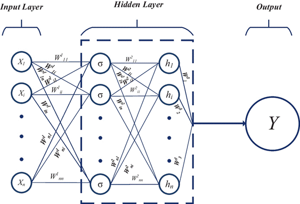
where x is the input vector, WL is the weight of the neuron layer of L, bL is the bias vector for layer L, fL() is the activation function for layer L, is the total number of layers, and  is the output of the model. After calculating the results of the weights (importance levels), the MLPRegressor comes to a singular output²⁶. This model was utilized in our research to see the outputs of a neural network compared to other, primarily tree-based models that split data between different decision-making branches.

XGBoost

The XGBoost model is a machine learning model with varying levels of decision trees within it, described by

   

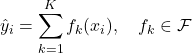
 is the predicted output of the sample, x_i is the input vector, f_k(x_i) is the prediction from the k tree, K is the total number of trees, f_k is the individual decision tree, x_i is the input features for the i data point, and F is the space of all possible regression trees. In XGBoost, each new decision tree is trained to correct the errors made by the ensemble of trees built so far and predictions are made by summing the results from each layer of trees and weighting them accordingly to arrive at a single outcome. Each tree adds more accuracy to the overall prediction. XGBoost was chosen to primarily compare previous models to a model that, at its core, uses gradient descent to consistently improve predictions.

Decision Tree Regressor

The Decision Tree Regressor is a nonlinear model illustrated by the equation:

   

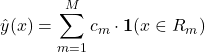
This equation represents the overall sum of the decisions made within the model to minimize model metrics in outputs. M is the number of leaf nodes, where the Decision Tree makes a prediction, Rm are the regions of data the model splits, and cm is the constant prediction of that leaf. x is the input. We tested the Decision Tree Regressor in an effort to analyze how an additional nonlinear model would perform against fairly linear data.

Training and Evaluation

The data was split into 5-fold cross validation subsets (20% each) following traditional data splitting guidelines for the best predictive outcomes, as more data leads to a better model, and is found that a 20% 5-fold split is often a good trade off between training and testing sets²⁷. We chose the subset splits using k-fold cross-validation, a method of model evaluation where the data is split into k folds. One of these folds is the validation fold, and the others are the training folds. The models are trained on the training folds and evaluated on the validation fold. The program then runs through every scenario in the k-fold iterations, meaning that after each validation evaluation, the validation fold changes until every training fold has been evaluated once. Then, the program averages the scores from the validation folds to produce the final metrics. In our pipeline, we utilized k-fold cross validation both before and after data engineering to see the extent of which data engineering was beneficial for model performance. We reported the accuracy of the different models using two error metrics: mean absolute error, and root mean squared error. The mean absolute error is similarly efficient in measuring model success because of its insensitivity to outliers and its simple interpretation, making it an effective but informative way of measuring error metrics. The root mean squared error penalizes larger errors more than smaller ones, increasing the population of lower, smaller error margins.

Results

Based on our results, we found that a Linear Regression model worked best with the dataset, along with the Ridge model. Having evaluated mean absolute error on both models, the Linear Regression model seemed to perform equivalent to the Ridge model, outperforming the other models with mean absolute errors of 17.96 ± 4.34. A Linear Regression model was particularly suitable for this task because of its low variance, meaning the model does not overfit easily and works well with fairly small datasets. In Figure 3, we compare the predictions of the Linear Regression model with the actual end prices of the auction. A perfect model would illustrate a graph of y = x.

The Ridge model was as effective and successful as the Linear Regression model; unlike Linear Regression, Ridge penalizes incorrect predictions and parameter values. The Ridge model only slightly performed better than the Linear Regression model, scoring a 17.96 ± 4.34 mean absolute error compared to Linear Regression’s 17.96 ± 4.34, a 37.17 ± 13.94 root mean squared error compared to Linear Regression’s 37.17 ± 13.93. By penalizing incorrect predictions that can help prevent overfitting, the model can thus be applied to different datasets and new statistical inputs²⁸. In this way, it accordingly minimizes the weight of irrelevant features in our dataset.

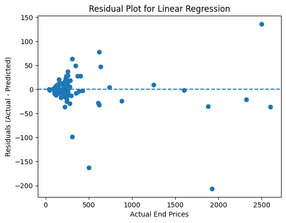
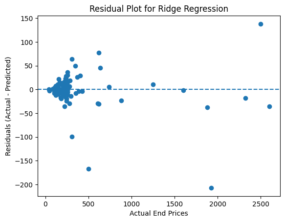
Both the Ridge and Linear Regression models demonstrated the highest accuracy among the models tested. The variety of the tested models ensures that we can visually measure which types of machine learning models perform the best in this predictive scenario. The variety of output calculation, including neural, tree-based, and linear models, tests all different model aspects of prediction. The understanding of nonlinearity and complex relationships is demonstrated through the predictions of the MLPRegressor, while the comprehension of irregular data and interactions between data is tested through the Random Forest Regressor and XGBoost. Algorithms oriented towards more straightforward and predictable trends are also tested through the Linear Regression and Ridge models.

Metric	Mean Absolute Error	Root Mean Squared Error
Linear Regression	90.85 ± 1.02	193.92 ± 14.59
Random Forest Regressor	49.28 ± 1.74	142.21 ± 12.05
Ridge	89.84 ± 1.18	194.24 ± 14.59
MLP Regressor	76.51 ± 1.57	176.90 ± 12.12
XGBoost	54.16 ± 2.55	148.84 ± 8.77
Decision Tree	57.22 ± 4.22	202.26 ± 12.40
Baseline (Mean Predictions)	234.22	444.37
Baseline (Opening + Avg Markup Predictions)	169.53	373.02

Metric	Mean Absolute Error	Root Mean Squared Error
Linear Regression	17.96 ± 4.34	37.17 ± 13.93
Random Forest Regressor	30.04 ± 11.35	84.04 ± 54.41
Ridge	17.96 ± 4.34	37.172 ± 13.94
MLP Regressor	20.26 ± 4.91	39.96 ± 14.77
XGBoost	28.77 ± 12.32	80.16 ± 60.01
Decision Tree	40.70 ± 12.51	106.07 ± 43.40
Baseline (Mean Predictions)	234.22	444.37
Baseline (Opening + Avg Markup Predictions)	169.53	373.02

Table 3 summarizes the performance metrics of each model using k-fold cross-validation before data engineering, while table 4 shows performance metrics using k-fold cross-validation after data engineering. Comparing table 3 and table 4, model performance drastically increased, with our top performing models after data engineering improving 56.25 and 71.88 mean absolute error points respectively, for the Ridge and Linear regression models. This drastic improvement could have happened because the engineered data revealed hidden relationships, allowing for more complex analysis and computation of the data. With more relationships to build on, the models have more connections to link to various outcomes, overall improving model performance. In the end, the Linear Regression and Ridge models worked best, as both models scored almost identical results, strongly outperforming other models. With the Linear Regression and Ridge models scoring 17.96 ± 4.34 and 17.96 ± 4.34, respectively, they outperformed the next best performing model by about two error metrics in both the mean absolute error and root mean squared error metrics. Comparatively to the two baseline predictors, the Linear Regression and Ridge models greatly outperformed baseline performance, demonstrating the improvement of predictions of the models from baseline accuracy. This means that both the Linear Regression and Ridge models would be extremely applicable in real predictive auction scenarios, allowing many to have a sense of final end prices on auctions.

One reason why the Ridge and Linear Regression models outperformed the other tested models could be because of the other models overfitting²⁹. This oftentimes happens when the training data is much larger and holds more information than the testing data, leading to models becoming more acclimated to memorizing outcomes rather than predicting end prices. Other models find high flexibility to noise and unrelated data, while Linear and Ridge regression do not.

Discussion

Throughout our work, we developed Linear Regression and Ridge models that can predict end prices of auctions for Cartier wristwatches, Palm Pilot M515 PDAs, and Xbox game consoles, within a 17 error metric range. This directly addressed our research objectives, as the model achieved a predictive accuracy of about 5.23% error, exact to our benchmark of a desired variation to within 5.23%. We came to this benchmark through finding the percentage error of an untuned Linear Regression model. We chose this model as a benchmark due to it being the strongest model available that could be implemented without unwanted complexity. The models performed essentially equal. We can deduce that the dataset was mostly linear, aiding Linear Regression in strong performance. Our aims served as a challenging yet achievable goal, and though this process required various code implementation and development, we were able to reach a proficient standard. Not only was the hypothesis met, but the model overachieved the goals we had set. This percentage of error is acceptable for real auction users, as the sub 10% error ensures that the model will predict accurately with minimal variation.

Though this research is fairly well-rounded, future work in this field would greatly benefit from a larger dataset, possibly with additional metrics such as time in between bids and the backgrounds of significant bidders and a larger variety of auction items³⁰. Additionally, it would be interesting to research how the error metrics of various models would perform when applied to data split into high-, medium-, and low-priced subdivisions of the overall auction data, to investigate whether or not the error varies with the target price. However, this research does provide a strong foundation for determining which machine learning method performed best. Based on this research, future research may proceed with an accurate, predetermined model to expand upon as appropriate to their situation³¹. Additionally, if the impact of typical personal preference for an item could be measured, it would provide a great deal of improvement for AI models. An emotion metric would allow models to determine the influence of attachment on customer bidding, further improving the end prediction.

Some individual limitations we faced in our work was having a limited variety of items being sold at auctions. If we had a larger variety of auctions being sold, our models could have been trained on much more data, increasing the overall accuracy of the end results and the applicability of the models. Furthermore, we lacked the emotional state of the participants, meaning the models did not have access to how the bidders felt when making bids at certain prices. This data would have been crucial to model development, as it would have allowed our models to make further relationships between the data in terms of emotion and financial activity.

Acknowledgments

Thank you to Omar Ramos Escoto, Victoria Lloyd and Inspirit AI for assisting me on this project.​ They were of much help throughout this process.

References

1. S. K. Reddy and M. Dass. “Modeling on-line art auction dynamics using functional data analysis.” Statistical Science. Vol. 21, no. 2, pp. 179–193, 2006. [↩]
2. P. W. Newberry. “The effect of competition on eBay.” International Journal of Industrial Organization. Vol. 40, pp. 107–118, 2015. [↩]
3. J. Zhang and H. Xu. “Auction design and bidder behavior: Understanding inequality in auction outcomes.” Proceedings of the AAAI Conference on Artificial Intelligence, 2022. [↩]
4. D. Ariely, A. Ockenfels, and A. E. Roth. “An experimental analysis of ending rules in internet auctions.” The RAND Journal of Economics. Vol. 36, no. 4, pp. 890–907, 2005. [↩]
5. A. Ockenfels and A. E. Roth. “Late and multiple bidding in second price Internet auctions: Theory and evidence concerning different rules for ending an auction.” Games and Economic Behavior. Vol. 55, no. 2, pp. 297–320, 2006. [↩]
6. A. E. Roth and A. Ockenfels. “Last-minute bidding and the rules for ending second-price auctions.” American Economic Review. Vol. 92, no. 4, pp. 1093–1103, 2002. [↩]
7. S. Lotz. Emotions in auctions: When and why bidders overbid. Doctoral dissertation, University of Mannheim, 2014. [↩]
8. S. Rafaeli and A. Noy. “Social presence and influence in online auctions.” Electronic Markets. Vol. 15, no. 2, pp. 158–175, 2005. doi:10.1080/10196780500083886. [↩]
9. D. Gefen and D. W. Straub. “Social presence and influence in online auctions.” Electronic Markets. Vol. 15, no. 2, pp. 131–138, 2005. [↩]
10. R. Bapna, P. Goes, and A. Gupta. “Analysis and design of business-to-consumer online auctions.” Management Science. Vol. 49, no. 1, pp. 85–101, 2003. [↩]
11. X. Li, Z. Lin, and Y. Li. “Predicting the final prices of online auction items.” IEEE International Conference on e-Business Engineering, 2006. [↩]
12. P. Bajari and A. Hortaçsu. “The winner’s curse, reserve prices, and endogenous entry: Empirical insights from eBay auctions.” The RAND Journal of Economics. Vol. 34, no. 2, pp. 329–355, 2003. doi:10.2307/1593721. [↩]
13. D. Nicholson and R. Paranjpe. A novel method for predicting the end-price of eBay auctions. CS229 Machine Learning Final Report, Stanford University, 2013. [↩] [↩]
14. W. Jank and G. Shmueli. Modeling Online Auctions. Wiley, 2010. [↩]
15. W. Wan and H.-H. Teo. “An examination of auction price determinants on eBay.” Proceedings of the 9th European Conference on Information Systems, 2001. [↩]
16. R. T. Wilcox. “Experts and amateurs: The role of experience in Internet auctions.” Marketing Letters. Vol. 11, no. 4, pp. 363–374, 2000. [↩]
17. P. Resnick and R. Zeckhauser. “Trust among strangers in internet transactions: Empirical analysis of eBay’s reputation system.” The Economics of the Internet and E-Commerce. Vol. 11, pp. 127–157, 2002. [↩]
18. M. I. Melnik and J. Alm. “Does a seller’s eCommerce reputation matter? Evidence from eBay auctions.” The Journal of Industrial Economics. Vol. 50, no. 3, pp. 337–349, 2003. [↩]
19. T. Firdose. “Filling missing values with mean and median.” Medium, 2023. [↩]
20. E. Haruvy and P. T. L. Popkowski Leszczyc. “The impact of online auction duration.” SSRN Electronic Journal, 2009. [↩]
21. H. M. Castro and J. C. Ferreira. “Linear and logistic regression models: When to use and how to interpret them?” Jornal Brasileiro de Pneumologia. Vol. 48, no. 6, 2023. doi:10.36416/1806-3756/e20220439. [↩] [↩]
22. D. F. Hamilton, M. Ghert, and A. H. Simpson. “Interpreting regression models in clinical outcome studies.” Bone & Joint Research. Vol. 4, no. 9, pp. 152–153, 2015. [↩]
23. J. Murel and E. Kavlakoglu. “What is ridge regression?” IBM, 2023. [↩]
24. “Ridge regression parameters.” OtasAI, 2024. [↩]
25. J. McCaffrey. “Regression using a scikit MLPRegressor neural network.” Visual Studio Magazine, 2023. [↩]
26. A. Kumar. “Sklearn neural network example – MLPRegressor.” Analytics Yogi, 2023. [↩]
27. A. Gholamy, V. Kreinovich, and O. Kosheleva. “Why 70/30 or 80/20 Relation Between Training and Testing Sets.” University of Texas at El Paso Technical Report TR-18-09, 2018. [↩]
28. H. Xu and S. Mannor. “Robustness and generalization.” arXiv, 2015. [↩]
29. “What is overfitting?” IBM, 2021. [↩]
30. R. Sehgal and F. T. Council. “AI needs data more than data needs AI.” Forbes, 2023. [↩]
31. T. Yarkoni and J. Westfall. “Choosing prediction over explanation in psychology: Lessons from machine learning.” PNAS. Vol. 116, no. 31, pp. 15849–15853, 2019. [↩]