Using Lifestyle Markers and Machine Learning to Detect Diabetes

Abstract

Diabetes is a prevalent chronic disease throughout the world and affects more than 100 million people just in the United States itself. Type 2 diabetes (T2D) can be prevented and controlled by managing lifestyle markers, such as diet and amount of exercise. In this project, a mathematical analysis of different lifestyle markers is presented along with a study using machine learning (ML) classifiers to detect prediabetes/diabetes cases. For this project, a dataset from the Centers for Disease Control and Prevention (CDC) containing 21 lifestyle markers (age, BMI, physical health, high blood pressure, etc.) and diagnosis of prediabetes/diabetes (binary label) from more than 250,000 adults was used. After conducting a comprehensive evaluation of several ML models (using 10-fold stratified cross-validation), it has been found that prediabetes/diabetes cases can be classified or detected with a high recall (>80%) using a Linear SVC model. In addition, this project presents an empirical relationship between lifestyle markers and their importance in the determination of diabetes by the model. A web application Diabetes Risk Analyzer has also been developed using the model trained in this project to detect prediabetes/diabetes based on lifestyle markers for use as a quick, robust, and widely accessible tool.

Keywords: diabetes, machine learning, supervised learning, classification

Introduction

Diabetes is a chronic disease that affects millions of people in the United States and the rest of the world. According to WHO, this chronic disease occurs when the pancreas does not produce enough insulin or when the body cannot use the insulin it produces effectively. By 2022, nearly 830 million people in the world were living with diabetes. In 2022, 14% of adults 18 years and older lived with diabetes. In 2021, diabetes was the direct cause of 1.6 million deaths and 47% of all deaths due to diabetes occurred before the age of 70 years. 

Diabetes can be divided into two categories, Type 1 diabetes (T1D) and Type 2 diabetes (T2D). More than 95% of people with diabetes have Type 2 diabetes (T2D). Type 2 diabetes was previously called non-insulin dependent or adult-onset. It prevents the body from using insulin properly, which can lead to high levels of blood sugar if not treated, and, over time, Type 2 diabetes can cause serious damage to the body, especially to nerves and blood vessels. Type 2 diabetes is often preventable. Factors that contribute to the development of type 2 diabetes include being overweight, not getting enough exercise, and genetics. Lifestyle changes are the best way to prevent or delay the onset of type 2 diabetes. Early diagnosis is important in preventing the worst effects of type 2 diabetes. In this project, the main contributions are the following: 

• Presenting the empirical relationship between different lifestyle markers, including their correlations and distributions between prediabetic/diabetic and nondiabetic populations. 

• Conducting a comprehensive evaluation of machine learning classifiers to detect prediabetes/diabetes using these lifestyle markers. This also includes identifying the top most influential markers for the model’s prediction. 

• Presenting a web application which uses the trained model in this project to detect prediabetes/diabetes based on the user’s current lifestyle markers.

While genetics and blood results can provide more comprehensive insights into the risk of diabetes for any individual, the scope of this project shows the screening potential using only lifestyle markers. Lifestyle markers are more widely available and easily accessible without incurring any medical tests or costs. An ML model is trained on the dataset used for this project in order to accurately classify prediabetes/diabetes cases based on lifestyle markers. 

Related work

In this paper¹, a machine learning model was trained to predict blood glucose levels using real-time data from monitored patients. Although this research and tool are useful for Type 1 diabetics, this applies only to patients already diagnosed with diabetes and insulin dependent. 

Similarly, in this paper², machine learning-based glucose prediction with the use of continuous glucose and physical activity monitoring data: The Maastricht study from the National Library of Medicine and machine learning is used to predict glucose levels accurately and safely based on continuous glucose monitoring (CGM). 

In this paper³, the authors have shown that physical activity is beneficial and can be used both for the management of Type 1 diabetes and for the prevention and management of Type 2 diabetes. Here too, it is emphasized that the presence of physical activity correlates with better physical and mental health. In addition, general health is one of the key attributes of the ML model in diagnosing diabetes. 

In this paper⁴, machine learning algorithms have also been used to diagnose diabetes with high precision. Here, the authors use a combination of lifestyle markers and medical information (insulin, glucose level, etc.) as input features for the ML models. However, medical measurements are not widely accessible to the general population and the determination of diabetes risk using such methods becomes limited. 

In this paper⁵, the authors have performed a similar analysis using the Receiver Operating Characteristic (ROC) on multiple data sets on diabetes. Their analysis spans only four machine learning classifiers, though, whereas this project covers the evaluation of eight machine learning classifiers.

In this paper⁶, six ML classifiers are evaluated using a dataset with only 768 data points consisting of eight markers (including BMI, age and clinical markers) and testset accuracies. 

In this paper⁷, three ML classifiers (logistic regression, naive bayes, adaboost) are evaluated on a dataset with lifestyle and clinical markers. 

 A key difference between this research paper and most related work on diabetes is that very few lifestyle markers have been explored for causative influence and correlation compared to this research, where 21 lifestyle markers from more than 250,000 adults were used.

Methods

Dataset

For this project, the CDC Diabetes Dataset from the UCI Machine Learning Repository was used. This dataset contains 253,680 data points, with 21 lifestyle markers (14 binary and 7 integer markers) pertaining to both men and women. 35,346 (=13.93%) cases are labeled as Yes (prediabetes/diabetes diagnosed) whereas the remaining 86.1% cases are labeled as No (prediabetes/diabetes not diagnosed). Table 1 below lists the different lifestyle markers to be used as input features for our model.

Feature	Type	Range	Description
Blood Pressure	Binary	0 – 1	0 indicates absence, 1 indicates presence.
Cholesterol	Binary	0 – 1	0 indicates absence, 1 indicates presence.
Cholesterol Check	Binary	0 – 1	0 indicates absence, 1 indicates presence.
Smoker	Binary	0 – 1	0 indicates absence, 1 indicates presence.
Stroke	Binary	0 – 1	0 indicates absence, 1 indicates presence.
Heart Disease or Attack	Binary	0 – 1	0 indicates absence, 1 indicates presence.
Physical Activity	Binary	0 – 1	0 indicates absence, 1 indicates presence.
Fruits	Binary	0 – 1	0 indicates absence, 1 indicates presence.
Veggies	Binary	0 – 1	0 indicates absence, 1 indicates presence.
Heavy Alcohol Consumption	Binary	0 – 1	0 indicates absence, 1 indicates presence.
Health Care	Binary	0 – 1	0 indicates absence, 1 indicates presence.
No Doctor Due to Cost	Binary	0 – 1	0 indicates absence, 1 indicates presence.
Walking Difficulty	Binary	0 – 1	0 indicates absence, 1 indicates presence.
Gender	Binary	0 – 1	0 = female 1 = male
BMI (kg/m2)	Integer	12 – 98	Body Mass Index in kg/m2
General Health	Integer	1 – 5	1 = excellent 2 = very good 3 = good 4 = fair 5 = poor
Mental Health	Integer	1 – 30	For how many days during the past 30 days was your mental health not good?
Physical Health	Integer	1 – 30	For how many days during the past 30 days was your physical health not good?
Age	Integer	1-13	13-level age category 1 (18-24 years) 2 (25-29 years) 3 (30-34 years) 4 (35-39 years) 5 (40-44 years) 6 (45-49 years) 7 (50-54 years) 8 (55-59 years) 9 (60-64 years) 10 (65-69 years) 11 (70-74 years) 12 (75-79 years) 13 (80+ years)
Education	Integer	1-6	Education level 1 (No school/only Kindergarten) 2 (Grades 1-8) 3 (Grades 9-11) 4 (High School Graduate) 5 (1-3 years of college) 6 (College Graduate)
Income	Integer	1-8	Income scale 1 (< $10,000) 2 ($10,000 – $15,000) 3 ($15,000-$20,000) 4 ($20,000-$25,000) 5 ($25,000-$35,000) 6 ($35,000-$50,000) 7 ($50,000-$75,000) 8 ($75,000+)

Age, Education, and Income are multi-category variables. Since their respective integer values correspond to intrinsic ordered ranges as shown in Table 1 above, we use these numeric values directly and do not use one hot encoding. This keeps our feature dimensionality low and avoids addition of sparse features.

These lifestyle markers play a vital role in the classification of prediabetes/diabetes cases. Using these lifestyle markers and the data from the dataset, the machine learning model chosen will be able to detect prediabetic/diabetic cases. 

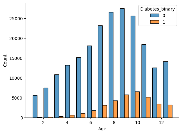
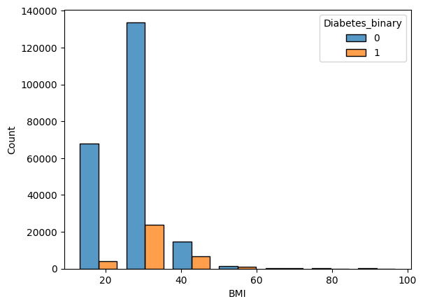
Figure 1 shows the distributions of the different age groups for the prediabetic/diabetic and non-diabetic population. For group 10 (ages⁸ 65-70), the count for diabetes peaks. Similarly, Figure 2 shows the distribution of BMI. Some lifestyle markers cannot be changed, such as gender and age, while others can be altered, such as intake of fruits, vegetables, and increase in physical activity. A Pearson correlation matrix, shown in Figure 3, was computed to explain and analyze the correlations between the different lifestyle markers.

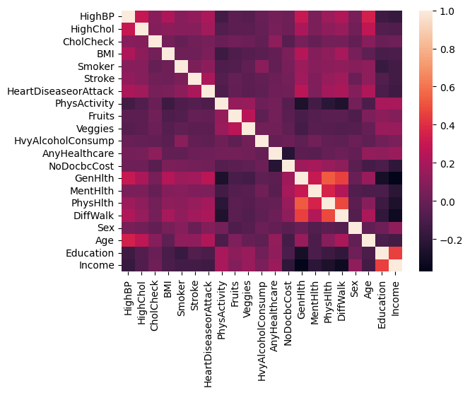
Cells in lighter colors show positive correlation, whereas cells in darker colors show negative correlation. This correlation matrix helps explain how lifestyle markers are related to each other. As shown in Figure 3, physical activity is negatively correlated with health markers (health markers in this dataset denote the number of days the patient’s health was not good). Hence, the presence of physical activity will influence good physical and mental health. Higher education and income groups also correlate with absence of high blood pressure, cholesterol, and low BMI. These are only rough measures and do not indicate full causal relationships. Table 2 depicts the mean and standard deviation for each feature, as shown below.

Feature	Training dataset (n=202944)	Validation dataset (n=25368)	Testing dataset (n=25368)
High Blood Pressure	0.429089 (0.494947)	0.427507 (0.494727)	0.429793 (0.495056)
High Cholesterol	0.424156 (0.494215)	0.423802 (0.494169)	0.424156 (0.494224)
Cholesterol Check	0.962561 (0.189835)	0.96468 (0.184591)	0.961526 (0.192341)
BMI	28.384303 (6.614076)	28.35872 (6.620453)	28.390492 (6.553833)
Smoker	0.442541 (0.496689)	0.441343 (0.496557)	0.450016 (0.497505)
Stroke	0.04044 (0.196989)	0.042179 (0.201002)	0.040011 (0.195989)
Heart Disease or Attack	0.094218 (0.292133)	0.096026 (0.294633)	0.092085 (0.289151)
Physical Activity	0.756036 (0.429472)	0.759618 (0.427324)	0.757529 (0.428586)
Fruits	0.634116 (0.481678)	0.635919 (0.481181)	0.633712 (0.481799)
Vegetables	0.811229 (0.391328)	0.809997 (0.392311)	0.814372 (0.388813)
Heavy Alcohol Consumption	0.056863 (0.231581)	0.053532 (0.225096)	0.053532 (0.225096)
Any Health Care	0.950986 (0.215897)	0.950173 (0.217591)	0.95246 (0.212795)
No Doctor Because of Cost	0.084477 (0.278102)	0.084989 (0.278871)	0.080968 (0.272792)
General Health	2.511038 (1.06769)	2.511944 (1.072901)	2.513679 (1.070379)
Mental Health	3.186037 (7.409267)	3.151766 (7.392514)	3.207663 (7.461807)
Physical Health	4.246462 (8.721475)	4.216138 (8.686586)	4.232971 (8.721354)
Difficulty Walking	0.168253 (0.374092)	0.165721 (0.371837)	0.17049 (0.37607)
Gender	0.439949 (0.496382)	0.444458 (0.496915)	0.439372 (0.49632)
Age	8.028776 (3.053709)	8.047304 (3.058033)	8.043677 (3.05454)
Education	5.051921 (0.984684)	5.04147 (0.993025)	5.047501 (0.9872)
Income	6.054931 (2.069851)	6.038789 (2.085603)	6.060509 (2.067018)

Table 2 summarizes the central tendency and variability of each lifestyle marker in the dataset by reporting the mean and standard deviation. 

Procedure

The original dataset was divided randomly into three mutually exclusive subsets⁹: a training set (80%), a validation set (10%), and a held-out test set (10%). The training set was used for model selection using cross-validation, the validation set was used for model operating point selection (threshold tuning) based on Receiver Operating Characteristic (ROC) analysis, and the testing set was used finally only once for reporting performance metrics. All these dataset splits were performed using stratified sampling¹⁰ to preserve the proportion of positive (prediabetes/diabetes) and negative cases across subsets. Feature standardization^11,12 (zero mean, unit variance) was fitted on the training data and applied to the validation and test sets to avoid data leakage. We use default hyperparameters from scikit-learn library for all model cross-validations or training.

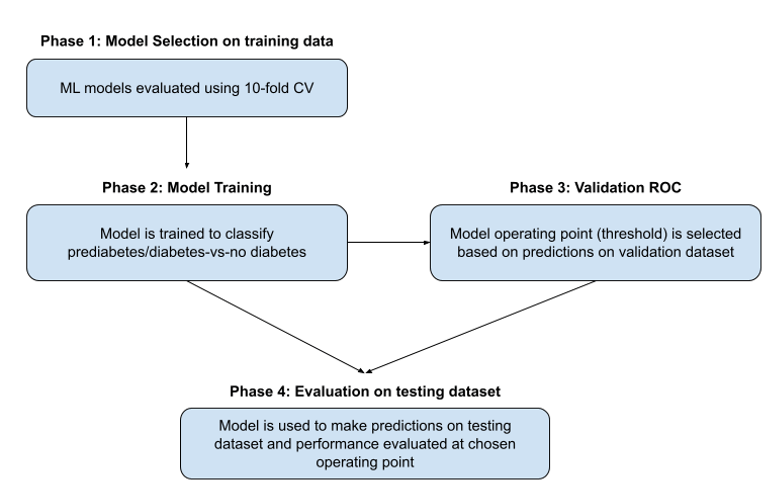
In this project, there were four main phases in the experimental project as shown in Figure 4. 

Phase 1: 10-fold stratified cross validation

In this phase, multiple ML classifiers were evaluated using 10-fold stratified cross-validation^13,14,15 (StratifiedKFold) with AUC (Area Under the ROC Curve) as the scoring metric on the training dataset. An AUC^16,17 close to 1 means the model effectively separates prediabetic/diabetic and non-diabetic cases well, while an AUC near 0.5 implies classification is almost random.  Stratified cross validation was used so that each fold has a similar proportion of prediabetic/diabetic and non-diabetic cases. Since the dataset is class-imbalanced (13.9% positive), model performance was evaluated using AUC. Scikit-learn, an API library for ML classifiers, was used for this purpose. Table 3 lists the eight different classifiers evaluated along with their AUC scores in ranked order. The Linear SVC model ranked highest with an AUC = 82.3% and was selected as the best model for this dataset and classification task. While Linear SVC, Logistic Regression¹⁸, and AdaBoost¹⁹ models performed similarly, Linear SVC (top-ranked) was selected for simplicity and interpretability. For all these models, we use default hyperparameters from scikit-learn.

ML Classifier Model	AUC
Linear SVC	82.30%
Logistic Regression	82.26%
AdaBoost	82.20%
Random Forest	79.84%
Naive Bayes	78.41%
QDA	78.06%
Nearest Neighbors	76.43%
Decision Tree	59.75%

Phase 2: Training

The Linear SVC model is then trained on the entire training dataset. For obtaining class probabilities, CalibratedClassifierCV was used with default parameters. The CalibratedClassifierCV uses cross-validation internally to both estimate the parameters of a classifier and subsequently calibrate a classifier. This is required since the LinearSVC model predicts only class labels and does not return class probabilities. 

Phase 3: Validation

In this phase, the trained Linear SVC model from Phase 2 makes predictions on the validation dataset. A Receiver Operating Characteristic (ROC) curve, depicting the relationship between the True Positive Rate (TPR) vs. the False Positive Rate (FPR), for the entire range of probability scores, is plotted for the validation dataset predictions. For this dataset, the Yes points (prediabetes/diabetes diagnosed) will be the positives and the No points (not diagnosed) will be the negatives. The True Positive Rate or Recall is defined as the ratio of the number of true positives (data points predicted correctly) by the model to the total number of positive data points. The False Positive Rate is defined as the ratio of the number of false positives (negative data points the model classified as positive), to the total number of negative data points. From the ROC plot, the optimal threshold is chosen as the operating point²⁰ of the model. This threshold represents a probability value, for classifying data points as positive with probability score above the threshold and Negative for data points scoring below the threshold.

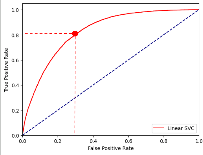
A conservative threshold of 0.1175 was chosen for the Linear SVC model, as shown by the red point in the ROC plot in Figure 5. A threshold of 0.1175 for the model corresponds to a true positive rate of 80.31% and a false positive rate of 31.71% on the validation dataset.

Phase 4: Testing 

In this phase, the trained Linear SVC model from Phase 2 makes predictions on the held-out testing dataset. The threshold selected from the validation set in Phase 3 is then applied without modification to the held-out test set to generate the final confusion matrix and performance metrics. The test set contains 25,368 individuals (3,534 with prediabetes/diabetes and 21,834 without).

Results

Linear SVC had the highest AUC, making it the optimal model for this project as shown in Table 3 above. A confusion matrix was created to depict the results based on the Linear SVC predictions on the testing dataset, as shown in Table 4 below. The test set contains 25,368 individuals (3,534 with prediabetes/diabetes and 21,834 without).

		Predicted label		Accuracy	70.08%
		No	Yes	Total	Recall
True label	No	14928	6906	21834	68.37%
	Yes	685	2849	3534	80.62%
	Total	15613	9755	25368
	Precision	95.61%	29.21%

Confusion matrices are utilized to depict the results of a machine learning classifier by comparing its predicted labels to the actual labels. The diagonal cells are the number of data points the model was able to correctly identify as positive or negative. The off-diagonal cells are the number of data points the model was not able to correctly predict. Overall, the model successfully achieved an accuracy of ~70%. In addition, the Linear SVC model was also able to achieve a 80.62% recall, which is more important, since the cost of classifying a non diabetic patient as prediabetic/diabetic is much less than the cost of classifying a prediabetic/diabetic patient as non diabetic. 

While prioritizing recall is most important for this project, the potential costs of false positives must be acknowledged as well. Potential costs include unnecessary anxiety for users, additional medical consultations, and possible strain on healthcare resources. Therefore, the model output should be interpreted strictly as a preliminary screening signal rather than a diagnostic result. In practice, any high-risk classification would need confirmation through standard clinical tests. The threshold value implemented reflects a deliberate trade-off favoring sensitivity over specificity to reduce missed cases, but different deployment contexts could justify alternative thresholds depending on acceptable false positive rates.

We also check how well calibrated are the model prediction probabilities as compared to the true outputs in the held-out testing dataset. The calibration curve²¹ is as shown below in Fig. 6.

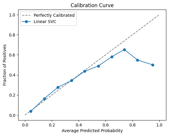
From Fig. 6, we find that the model scores are well-calibrated up to probability = 0.5 after which the model is over-predicting. For our classification context, we are using a conservative threshold of 0.1175 only to flag prediabetic/diabetic cases. We are not using these model prediction probabilities as risk scores.

Performance is also evaluated on different subsets of the testing dataset:

• Young adults: For this subset, the age groups 1 and 2 corresponding to populations with ages 18-24 and 25-29 respectively in the testing dataset are evaluated. There are 1,286 cases here with only 2% labeled as prediabetics/diabetics. The Linear SVC model still achieves a recall of ~42% for the positive class and an overall accuracy of 95%.

		Predicted label		Accuracy	95.10%
		No	Yes	Total	Recall
True label	No	1213	49	1262	96.12%
	Yes	14	10	24	41.67%
	Total	1227	59	1286
	Precision	98.86%	16.95%

• Men: For this subset, the male population in the testing dataset is evaluated. There are 11,208 cases here with 15.27% of prediabetics/diabetics. Recall for the positive class is ~81%, which is very similar to that of the entire testing dataset (=80.62%). Overall accuracy is 67.58%, which is slightly less than overall accuracy of entire testing dataset (=70.08%)

		Predicted label		Accuracy	67.58%
		No	Yes	Total	Recall
True label	No	6193	3303	9496	65.22%
	Yes	331	1381	1712	80.67%
	Total	6524	4684	11208
	Precision	94.93%	29.48%

• Women: For this subset, the female population in the testing dataset is evaluated. There are 14,160 cases here with 12.87% of prediabetics/diabetics. Recall for the positive class is ~81%, which is very similar to the male population recall and that of the entire testing dataset (=80.62%). Overall accuracy is 72.06%, which is more than overall accuracy of male population (=67.58%) and slightly more than that of the entire testing dataset (= 70.08%).

		Predicted label		Accuracy	72.06%
		No	Yes	Total	Recall
True label	No	8735	3603	12338	70.80%
	Yes	354	1468	1822	80.57%
	Total	9089	5071	14160
	Precision	96.11%	28.95%

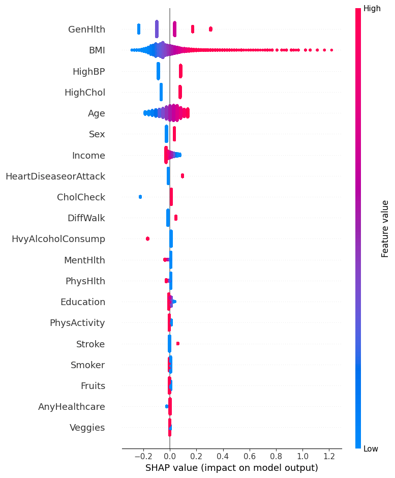
SHAP Analysis

A SHapley Additive exPlanations (SHAP) plot was created to explain which lifestyle markers most strongly influenced the model prediction output, as shown in Figure 7. SHAP is a library that can attribute the overall contribution of each lifestyle marker to the final prediction. General health, BMI, and High BP are the strongest contributors for the final decision from the Linear SVC model. The purpose of this SHAP^22,23,24 plot is to quantitatively measure the contributions each lifestyle marker had on the prediction of the model, essentially providing a ranked list of the most influential markers. For General health, the range of values correspond to 1 = excellent, 2 = very good, 3 = good, 4 = fair and 5 = poor. According to the SHAP plot, higher BMI²⁵, poorer general health (higher values), and HighBP²⁶ (=1) increased the predicted model score, whereas lower BMI, HighBP (=0), and better general health (lower values) decreased it.

Here are some data examples from the validation dataset in the following Table 8 for some current prediabetic/diabetic cases. Table 9 shows the corresponding SHAP feature contributions.

HighBP	BMI	GenHlth	Gender	Age	Label
1	28	5	1	9	1
1	34	2	0	10	1
1	50	4	0	8	1

HighBP	BMI	GenHlth	Gender	Age	Max factor
0.0808	-0.0351	0.3077	0.0341	0.0278	GenHlth
0.0808	0.0724	-0.0989	-0.0257	0.0545	HighBP
0.0808	0.3592	0.1721	-0.0257	0.0011	BMI

All of the code was developed in Python on Google’s Colab notebook and is available on GitHub.

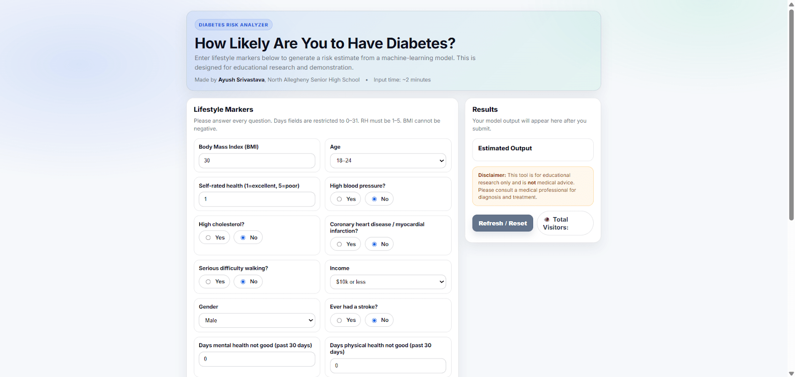
Web application

The web application created utilizes a Flask server hosting the trained Linear SVC model in the back-end. Users enter their lifestyle markers, which are then passed to the model for predictions. Based on the lifestyle markers of the user, the model outputs “HIGH” if the prediction is above the chosen threshold of 0.1175 and “LOW” if the prediction is below the chosen threshold, as shown in Figure 8. While this web application aims to provide users with their classification of prediabetes/diabetes, it does not aim to provide medical advice or replace professional medical diagnosis. This is only for preliminary screening use only. This web application is deployed on AWS and it does not log or store any users’ data (form entries) or IP addresses. The user inputs are only passed to the model for prediction purposes.

Discussion

In conclusion, the Linear SVC model was able to achieve an 80.62% prediabetes/diabetes classification recall on the held-out testing dataset, comprising 10% of the total dataset. While this was a single‐dataset and multiple‐split evaluation conducted, external validation is future work. A trivial baseline classifying all individuals as non-diabetic would achieve ~86% accuracy but 0% recall for the positive class, demonstrating the need for a recall-oriented model.

A web application was created where the trained Linear SVC model can make a prediabetes/diabetes classification using the user’s input lifestyle markers. This project met all the objectives of an accurate model, a mathematical analysis, and the web application. 

The first objective, which was to train a machine learning classifier to accurately differentiate between positive cases and negative cases, was achieved through the selection of the best classifier, the training procedure of the model, and the optimal threshold chosen. 

The second objective, which was to analyze and explain which lifestyle markers were the most correlated with prediabetes/diabetes, was achieved by computing the SHAP plot and the correlation matrix. Both of these diagrams assist in the analysis and explanation of the model’s predictions. 

Lastly, the web application can be utilized to make quick, robust, and accessible prediabetes/diabetes classifications. Our model is not replacing any official test; it is an extra early warning using lifestyle only. In real clinics, a high‐risk flag would still need a blood test. Also, this model is mostly suited to populations similar to the CDC dataset, and its performance on other countries is still unknown or a future work. Some future goals with this project are to evaluate this model on more global diabetes datasets, such as the PIMA Indians Diabetes Database. 

References

1. A. Devi, P. Sasireka, K. Kovardhani, G. Premalatha, T. Sivasakthi and R. Subash, “Blood Glucose Diabetic Prediction using Machine Learning Algorithm,” 2024 2nd International Conference on Sustainable Computing and Smart Systems (ICSCSS), Coimbatore, India, 2024, pp. 1519-1522, doi: 10.1109/ICSCSS60660.2024.10625217. keywords: {Machine learning algorithms;Accuracy;Vectors;Diabetes;Glucose;Biosensors;Biomedical monitoring;Diabetes;Decision Trees;Machine Learning;Random Forests;Support Vector Machines} URL https://ieeexplore.ieee.org/document/10625217. [↩]
2. W. PTM Van Doorn, Y.D Foreman, N C Schaper, Hans HCM Savelberg, Annemarie Koster, Carla JH van der Kallen, Anke Wesselius, Miranda T Schram, Ronald MA Henry, Pieter C Dagnelie, et al. Machine learning-based glucose prediction with use of continuous glucose and physical activity monitoring data: The maastricht study. PloS one, 16(6):e0253125, 2021. URL https://doi.org/10.1371/journal.pone.0253125. [↩]
3. C. Hayes and A. Kriska. Role of physical activity in diabetes management and prevention. Journal of the American Dietetic Association, 108(4):S19–S23, 2008. URL https://doi.org/10.1016/j.jada.2008.01.016. [↩]
4. A. Mujumdar and V. Vaidehi. Diabetes prediction using machine learning algorithms. Procedia Computer Science, 165:292–299, 2019. ISSN 1877- 0509. doi: https://doi.org/10.1016/j.procs.2020.01.047. URL https://www.sciencedirect.com/science/article/pii/S1877050920300557. 2nd International Conference on Recent Trends in Advanced Computing ICRTAC -DISRUP – TIV INNOVATION , 2019 November 11-12, 2019. [↩]
5. Hang Lai, Huaxiong Huang, Karim Keshavjee, Aziz Guergachi, and Xin Gao. Predictive models for diabetes mellitus using machine learning techniques. BMC endocrine disorders, 19:1–9, 2019. URL https://doi.org/10.1186/s12902-019-0436-6. [↩]
6. Abdulhadi, Nour, and Amjed Al-Mousa. “Diabetes detection using machine learning classification methods.” 2021 international conference on information technology (ICIT). IEEE, 2021. URL https://doi.org/10.1109/ICIT52682.2021.9491788 [↩]
7. Mijwil, Maad M., and Mohammad Aljanabi. “A comparative analysis of machine learning algorithms for classification of diabetes utilizing confusion matrix analysis.” Baghdad Science Journal 21.5 (2024): 24. URL https://doi.org/10.21123/bsj.2023.9010 [↩]
8. Nanayakkara, Natalie, et al. “Impact of age at type 2 diabetes mellitus diagnosis on mortality and vascular complications: systematic review and meta-analyses.” Diabetologia 64.2 (2021): 275-287. URL https://doi.org/10.1007/s00125-020-05319-w [↩]
9. Burzykowski, Tomasz, et al. “Validation of machine learning algorithms.” American journal of orthodontics and dentofacial orthopedics 164.2 (2023): 295-297. URL https://www.ajodo.org/article/S0889-5406(23)00260-3/pdf [↩]
10. Khushi, Matloob, et al. “A comparative performance analysis of data resampling methods on imbalance medical data.” Ieee Access 9 (2021): 109960-109975. URL https://doi.org/10.1109/ACCESS.2021.3102399 [↩]
11. Mathivanan, Norsyela Muhammad Noor, et al. “Impact Of Feature Standardization On Heart Disease Prediction: A Comparative Analysis Of Logistic Regression And Support Vector Machine Models.” Malaysian Journal of Computing 10.2 (2025): 2159-2175. URL https://journal.uitm.edu.my/ojs/index.php/MJoC/article/download/6835/4908 [↩]
12. Sujon, Khaled Mahmud, et al. “When to use standardization and normalization: Empirical evidence from machine learning models and XAI.” IEEE access 12 (2024): 135300-135314. URL https://doi.org/10.1109/ACCESS.2024.3462434 [↩]
13. Yates, Luke A., et al. “Cross validation for model selection: a review with examples from ecology.” Ecological monographs 93.1 (2023): e1557. URL https://doi.org/10.1002/ecm.1557 [↩]
14. Stephen Bates, Trevor Hastie & Robert Tibshirani (2024) Cross-Validation: What Does It Estimate and How Well Does It Do It?, Journal of the American Statistical Association, 119:546, 1434-1445, URL https://doi.org/10.1080/01621459.2023.2197686 [↩]
15. Sweet, Lily-belle, et al. “Cross-validation strategy impacts the performance and interpretation of machine learning models.” Artificial Intelligence for the Earth Systems 2.4 (2023): e230026. URL https://journals.ametsoc.org/downloadpdf/view/journals/aies/2/4/AIES-D-23-0026.1.pdf [↩]
16. Polo TCF, Miot HA. Use of ROC curves in clinical and experimental studies. J Vasc Bras. 2020;19: e20200186. URL https://doi.org/10.1590/1677-5449.200186 [↩]
17. Yang, Tianbao, and Yiming Ying. “AUC maximization in the era of big data and AI: A survey.” ACM computing surveys 55.8 (2022): 1-37. URL https://dl.acm.org/doi/pdf/10.1145/3554729 [↩]
18. Zabor, Emily C., et al. “Logistic regression in clinical studies.” International Journal of Radiation Oncology* Biology* Physics 112.2 (2022): 271-277. URL https://doi.org/10.1016/j.ijrobp.2021.08.007 [↩]
19. Shahraki, Amin, Mahmoud Abbasi, and Øystein Haugen. “Boosting algorithms for network intrusion detection: A comparative evaluation of Real AdaBoost, Gentle AdaBoost and Modest AdaBoost.” Engineering Applications of Artificial Intelligence 94 (2020): 103770. URL https://doi.org/10.1016/j.engappai.2020.103770 [↩]
20. Hassanzad, Mojtaba, and Karimollah Hajian-Tilaki. “Methods of determining optimal cut-point of diagnostic biomarkers with application of clinical data in ROC analysis: an update review.” BMC medical research methodology 24.1 (2024): 84. URL https://link.springer.com/content/pdf/10.1186/s12874-024-02198-2.pdf [↩]
21. Austin, Peter C., Frank E. Harrell Jr, and David van Klaveren. “Graphical calibration curves and the integrated calibration index (ICI) for survival models.” Statistics in Medicine 39.21 (2020): 2714-2742. URL https://doi.org/10.1002/sim.8570 [↩]
22. Mosca, Edoardo, et al. “SHAP-based explanation methods: a review for NLP interpretability.” Proceedings of the 29th international conference on computational linguistics. 2022. URL https://aclanthology.org/2022.coling-1.406.pdf [↩]
23. Ponce‐Bobadilla, Ana Victoria, et al. “Practical guide to SHAP analysis: Explaining supervised machine learning model predictions in drug development.” Clinical and translational science 17.11 (2024): e70056. URL https://doi.org/10.1111/cts.70056 [↩]
24. Wang, Huanjing, et al. “Feature selection strategies: a comparative analysis of SHAP-value and importance-based methods.” Journal of Big Data 11.1 (2024): 44. URL  https://doi.org/10.1186/s40537-024-00905-w [↩]
25. Chandrasekaran, Preethi, and Ralf Weiskirchen. “The role of obesity in type 2 diabetes mellitus—An overview.” International journal of molecular sciences 25.3 (2024): 1882. URL https://doi.org/10.3390/ijms25031882 [↩]
26. Naseri, Mohammad Wali, Habib Ahmad Esmat, and Mohammad Daud Bahee. “Prevalence of hypertension in Type-2 diabetes mellitus.” Annals of Medicine and Surgery 78 (2022). URL https://doi.org/10.1016/j.amsu.2022.103758 [↩]