Simulating Incompressible Fluid Flow in a 2D Channel: From Poiseuille’s Law to Realistic Navier-Stokes Solutions

March 30, 2026

Abstract

This study uses numerical simulations to investigate incompressible viscous fluid flow in a two-dimensional (2D) channel, beginning with the ideal laminar case described by planar Poiseuille’s flow and extending to more complex geometries with constrictions, wall roughness, and suspended particles. A 2D incompressible Navier–Stokes solver was implemented to explore the effects of channel constrictions, wall roughness, and varying Reynolds numbers. The simulations reproduce the classical parabolic velocity profile in smooth channels and reveal how constrictions generate jet-like acceleration, recirculation zones, and vortex shedding. Quantitative analysis shows that flow resistance and energy dissipation rise with both Reynolds number and constriction severity, while sharp step-like constrictions amplify vortex shedding compared to smooth Gaussian ones, with hydraulic resistance governed by both local dissipation and downstream pressure recovery. A simplified Lagrangian particle transport was also modeled, highlighting inertial focusing on low Reynolds numbers and increased wall deposition at higher Reynolds numbers, especially near constrictions. These results illustrate how channel imperfections and flow instabilities contribute to energy losses and particle accumulation. Extension to real-world applications, such as blood flow in vascular vessels or fluid transport in pipelines, would require fully 3D modeling and substantially more sophisticated and computationally intensive simulations.

Keywords: Fluid dynamics, Navier-Stokes equations, rectangular channel, Reynolds number, laminar flow, vortex shedding, sedimentation

Introduction

Fluid dynamics governs how liquids and gases move, from phenomena like water flow in channels, air around airplane wings to ocean currents. The mathematical models to describe the motion of viscous fluid substances were developed in the 19th century as the Navier-Stokes equations, by applying Newton’s second law to fluid, accounting for viscosity, pressure, and external forces¹^,². They are a set of partial differential equations (PDE), however, are notoriously difficult to solve analytically due to their nonlinear and coupled nature. The nonlinear convective term in the equation causes chaotic behavior, i.e. the solution is highly sensitive to initial conditions. The velocity and pressure fields are interdependent, making the system a set of coupled PDEs. In 2000, the Clay Mathematics Institute designated the Navier-Stokes existence and smoothness problem as one of its seven Millennium Prize Problems³.

While the general analytical solutions to Navier-Stokes equations are still elusive and probably non-existing in 3D, there are a few simple cases with existing analytical solutions by some assumptions of steady-state, incompressibility, and certain symmetry to simplify the equations⁴. Laminar flow is one of the simplest types of fluid motion. It occurs when a fluid flows in parallel layers, with minimal mixing and no turbulence. The velocity field in the steady state is described by Poiseuille’s law⁵. Real-world pipes, however, like blood vessels or industrial pipelines, have imperfections such as constrictions and rough surfaces⁶. Flows may become unsteady or turbulent and result in large pressure drops along the channels and energy losses.

This study investigated fluid flow in a channel by starting with planar Poiseuille’s flow and progressively adding complexity to approach realistic scenarios. Using numerical simulations by a full 2D Navier-Stokes solution without the laminar assumption, we modeled: (1) laminar flow in an ideal smooth no-slip channel that a parabolic velocity profile is developed in the channel regardless of Re numbers (2) vortex shedding which deviate from laminar flow with different shapes of constrictions and random roughness (3) particle transport and deposition in the flow to study clogging at constrictions under varying Re numbers. The research is to understand: How channel imperfections and unsteady effects can alter flow compared to the ideal Poiseuille case, and how these changes contribute to energy losses, and reveal about the Navier-Stokes equations’ complexity. The combined analytical and numerical methods explore ideal and realistic flow scenarios in 2D. We emphasize that understanding and accurately simulating real-world systems, such as blood flow in affected vessels or viscous fluid transport in complex pipelines, would require fully 3D modeling and substantially more computationally intensive methods.

Navier-Stokes Equations

We start by introducing the Navier-Stokes equations for an incompressible fluid:

Momentum Equation:

(1) $\begin{equation*}\frac{\partial \mathbf{u}}{\partial t} + \mathbf{u} \cdot \nabla \mathbf{u} = -\frac{1}{\rho}\nabla p + \nu \nabla^2 \mathbf{u} + \mathbf{G}\end{equation*}$

Continuity Equation:

(2) $\begin{equation*}\nabla \cdot \mathbf{u} = 0\end{equation*}$

Here:

$\mathbf{u} = (u_x, u_y, u_z)$ : Velocity vector field of the fluid.
$t$ : Time. %
$\rho$ : Density of fluid.
$p$ : Pressure field.
$\nu$ : Kinematic viscosity of fluid.
$\mathbf{G}$ : External forces.
$\nabla$ : Gradient operator.
$\nabla^2$ : Laplacian operator.
$\mathbf{u} \cdot \nabla \mathbf{u}$ : Convective term.

The equations describe how the velocity, pressure and density of a fluid evolve over time and space.
It is instructive to understand each term in the momentum equation: $\frac{\partial \mathbf{u}}{\partial t}$ is the rate of change of the velocity field or acceleration of fluid particles;
$\mathbf{u} \cdot \nabla \mathbf{u}$ is the nonlinear convective term, representing how the fluid’s velocity transports itself, leading to complex behaviors like turbulence;
$-\frac{1}{\rho}\nabla p$ is the pressure gradient force, driving fluid from high to low pressure;
$\nu \nabla^2 \mathbf{u}$ is the viscous term, modeling the diffusion of momentum due to viscosity;
$\mathbf{G}$ is external forces, such as gravity or electromagnetic forces.
The continuity equation ensures mass conservation, i.e. for an incompressible fluid, the volume of fluid entering a region equals the volume leaving it⁴.

Poiseuille’s Law

Poiseuille’s Law is a specific solution to Navier-Stokes equations under simplified conditions for laminar flow in a planar channel⁷. The laminar flow is in steady state and moving in parallel layers, so $\frac{\partial \mathbf{u}}{\partial t} = 0$ and $\mathbf{u} \cdot \nabla \mathbf{u} = 0$ .
The velocity field in a planar channel does not change along the channel’s length, only varying radially, therefore, in a planar coordinate $(r, z)$ , the velocity field $\mathbf{u} = (u_r, u_z) = (u(r), 0)$ , where $r$ is the radial distance from the channel center, $z$ is the axial direction along the channel.
Pressure only varies along $z$ with a constant pressure gradient $\frac{\partial p}{\partial z} = -\frac{\Delta P}{L}$ and there are no external forces along the channel.

The Navier-Stokes equation in the z-direction becomes:

(3) $\begin{equation*}0 = \frac{\Delta P}{L} + \mu \frac{1}{r} \frac{\partial}{\partial r} \left(r \frac{\partial u}{\partial r}\right)\end{equation*}$

Rearrange the equation:

(4) $\begin{equation*}\frac{\partial}{\partial r} \left(r \frac{\partial u}{\partial r}\right) = -\frac{\Delta P}{\mu L} r\end{equation*}$

Integrate with respect to r:

(5) $\begin{equation*}r \frac{\partial u}{\partial r} = -\frac{\Delta P}{2\mu L} r^2 + C_1\end{equation*}$

(6) $\begin{equation*}\frac{\partial u}{\partial r} = -\frac{\Delta P}{2\mu L} r + \frac{C_1}{r}\end{equation*}$

To avoid singularity at $r=0$ , set the constant $C_1=0$ :

(7) $\begin{equation*}\frac{\partial u}{\partial r} = -\frac{\Delta P}{2\mu L} r\end{equation*}$

Integrate again:

(8) $\begin{equation*}u = -\frac{\Delta P}{4\mu L} r^2 + C_2\end{equation*}$

Apply the no-slip boundary condition $u(R)=0$ at the channel wall:

(9) $\begin{equation*}0 = -\frac{\Delta P}{4\mu L} R^2 + C_2\end{equation*}$

We obtain the parabolic velocity profile for laminar flow in a channel:

(10) $\begin{equation*}u(r) = \frac{\Delta P}{4\mu L} (R^2 - r^2)\end{equation*}$

The Poiseuille’s Law describes the relationship between volume flow rate and pressure drop of laminar flow through a long planar channel and is therefore obtained by integrating the above equation over the channel’s cross-sectional area:

(11) $\begin{equation*}Q = \int_0^R u(r) \cdot 2\pi r \, dr = \int_0^R \frac{\Delta P}{4\mu L}(R^2 - r^2) \cdot 2\pi r \, dr = \frac{\pi \Delta P R^4}{8\mu L}\end{equation*}$

Poiseuille’s law strictly applies only to steady, fully developed flow in constant-width channels.
It is therefore not applied within constricted or varying-width regions of the channel.

Full 2D Navier-Stokes Simulation

Analytical solution to the Navier-Stokes equations is difficult, however, the numerical methods and approximations allow engineers and scientists to use the Navier-Stokes equations effectively to study fluid dynamics in complex geometries as in aerodynamics and weather modeling.
Without going to the full extent to simulate the fluid flow in 3D, which might require commercial software and significant computational power, we solve the incompressible Navier-Stokes equations in a 2D rectangular channel, which represents a cut-away view of a pipeline, with different shapes of constrictions and random wall roughness, to capture time-dependent and turbulence-like effects.

The incompressible Navier-Stokes equations in 2D are:

Momentum equation:

(12) $\begin{equation*}\frac{\partial u_x}{\partial t} + u_x\frac{\partial u_x}{\partial x} + u_y\frac{\partial u_x}{\partial y} = -\frac{1}{\rho}\frac{\partial p}{\partial x} + \nu\left(\frac{\partial^2 u_x}{\partial x^2} + \frac{\partial^2 u_x}{\partial y^2}\right) + G_x\end{equation*}$

(13) $\begin{equation*}\frac{\partial u_y}{\partial t} + u_x\frac{\partial u_y}{\partial x} + u_y\frac{\partial u_y}{\partial y} = -\frac{1}{\rho}\frac{\partial p}{\partial y} + \nu\left(\frac{\partial^2 u_y}{\partial x^2} + \frac{\partial^2 u_y}{\partial y^2}\right) + G_y\end{equation*}$

Continuity equation:

(14) $\begin{equation*}\frac{\partial u_x}{\partial x} + \frac{\partial u_y}{\partial y} = 0\end{equation*}$

The external body force $\mathbf{G} = (G, 0)$ is applied in the x-direction and serves as the driving force to induce and sustain the fluid flow through the channel, which is equivalent to a constant pressure gradient and central to Poiseuille’s Law.
This is a common numerical technique in computational fluid dynamics (CFD) simulations of channel or Poiseuille-like flows.
If without non-zero $G$ in simulation and the simulation starts from rest, $u_x = u_y = 0$ , the velocities will remain zero indefinitely, as there’s nothing to initiate motion and the flow would be stagnant with no time evolution.

In incompressible channel flow, a constant streamwise body force $f_x$ is mathematically equivalent to a constant pressure gradient.
Specifically, imposing a uniform body force $f_x$ is equivalent to imposing a constant pressure gradient satisfying

(15) $\begin{equation*}\frac{1}{\rho} \frac{\partial p}{\partial x} = -f_x\end{equation*}$

Therefore, although the numerical implementation uses a body-force formulation rather than explicit pressure boundary conditions, the flow is physically pressure-driven.
This approach is standard in computational studies of Poiseuille and channel flows and avoids complications associated with pressure boundary specification while preserving the correct momentum balance.

In the early 20th century, the Stream Function–Vorticity formulation emerged, e.g. in Horace Lamb’s Hydrodynamics 1879, as an alternative way to write the Navier–Stokes equations. It is particularly useful for 2D incompressible flows.
It simplifies the equations by eliminating the pressure term by working with vorticity ( $\omega$ ) and automatically satisfying continuity equation using a stream function ( $\psi$ )

The stream function is defined such that the continuity is satisfied automatically:

(16) $\begin{equation*}u_x = \frac{\partial \psi}{\partial y}, \quad u_y = -\frac{\partial \psi}{\partial x}\end{equation*}$

Vorticity is the curl of the velocity field to measure rotation:

(17) $\begin{equation*}\omega = \frac{\partial u_y}{\partial x} - \frac{\partial u_x}{\partial y}\end{equation*}$

We can therefore plug in $u_x, u_y$ from stream function to get the Poisson equation connecting $\omega$ and $\psi$ :

(18) $\begin{equation*}\omega = \frac{\partial}{\partial x}\left(-\frac{\partial \psi}{\partial x}\right) - \frac{\partial}{\partial y}\left(\frac{\partial \psi}{\partial y}\right) = -\left(\frac{\partial^2 \psi}{\partial x^2} + \frac{\partial^2 \psi}{\partial y^2}\right) = -\nabla^2 \psi\end{equation*}$

Take the curl of both sides of Navier-Stokes equation:

(19) $\begin{equation*}\nabla \times \left( \frac{\partial \mathbf{u}}{\partial t} + \mathbf{u} \cdot \nabla \mathbf{u} \right) = \nabla \times \left( -\frac{1}{\rho}\nabla p + \nu \nabla^2 \mathbf{u} + \mathbf{G} \right)\end{equation*}$

Apply curl properties and obtain the vorticity transport equation:

(20) $\begin{equation*}\frac{\partial \omega}{\partial t} + \mathbf{u} \cdot \nabla \omega = \nu \nabla^2 \omega\end{equation*}$

In 2D:

(21) $\begin{equation*}\frac{\partial \omega}{\partial t} + u_x \frac{\partial \omega}{\partial x} + u_y \frac{\partial \omega}{\partial y} = \nu \left( \frac{\partial^2 \omega}{\partial x^2} + \frac{\partial^2 \omega}{\partial y^2} \right)\end{equation*}$

In terms of physical meaning, vorticity represents the curl of the velocity field and quantifies the local angular velocity of fluid elements.
It can reveal fine-scale structures that might be invisible in velocity field plot for detection of turbulent transitions.
Streamlines are tangent to the velocity vector of the fluid and represent the paths a massless particle would flow.

Though streamfunction and vorticity have their clear and intuitive physical meaning, the numerical solver employed in this study is not a streamfunction–vorticity formulation.
The incompressible Navier–Stokes equations are advanced in time using a projection method in primitive variables $(u_x, u_y, p)$ .
The streamfunction $\psi$ and vorticity $\omega$ fields are computed only in post-processing from the velocity field for visualization purposes.
As a result, no vorticity boundary conditions are imposed or required in the numerical time stepping.

Boundary Conditions

The simulations are performed in a two-dimensional channel of length $L_x$ and height $H$ . Periodic boundary conditions are imposed in the stream $x$ direction for both velocity and pressure fields, consistent with a spatially repeating channel segment. In the wall-normal $y$ direction, no-slip and impermeable boundary conditions are enforced on the top and bottom walls, such that

(22) $\begin{equation*}\mathbf{u} = (0, 0) \quad \text{on } y=0 \text{ and } y=H\end{equation*}$

Channel imperfections and obstacles are modeled as solid walls. No-slip and no-penetration conditions are imposed on all obstacle boundaries.

The flow is driven by a uniform body-force term in the stream direction, which is equivalent to a constant mean pressure gradient in a periodic domain.

Reynolds Number

The Reynolds number (Re) is a dimensionless quantity in fluid dynamics. It compares the relative importance of inertial forces to viscous forces in the fluid. It is defined as:

(23) $\begin{equation*}Re = \frac{\rho U L}{\mu} = \frac{U L}{\nu} \end{equation*}$

where $\rho$ is the fluid density, U is a characteristic velocity (e.g., mean or maximum flow speed), L is a characteristic length scale (e.g., channel height or pipe diameter), $\mu$ is the dynamic viscosity, and $\nu$ is the kinematic viscosity.

In the case of channel flow, Re is often computed using the centerline velocity and half-channel height as $Re = \frac{G H^3}{16\nu^2}$ (where G is the driving force of the flow and H is the full channel height).

Physically, Re is used to characterize the nature of fluid flow:

a) Laminar Flow: Typically occurs at low Re, $Re < 2,000$ for channel flow. The flow is smooth, with fluid moving in parallel layers where viscous forces dominate. b) Transitional Flow: Occurs at intermediate Re, e.g., $2,000 < Re < 4,000$ , where the flow can change between laminar and turbulent. c) Unsteady separated flow: can occur at high Re, e.g., $Re > 5,000$ .

This is the region where inertial forces prevail, leading to irregular motion and eddies in the flow⁸ It enables similarity analysis for results from models on different scales but similar Re number.

This is essential in aerospace, automotive, and civil engineering for designing efficient systems without full-scale prototyping. Therefore, in our simulation Re is used as a control parameter to characterize different classes of flows from laminar to unsteady flow.

Nondimensionalization

To express the governing equations and simulation results in a general, scale-independent form, all variables are nondimensionalized using characteristic reference quantities.
Length is scaled by the full channel height $H$ , velocity by a reference velocity $U_{ref}$ , and pressure by $\rho U_{ref}^2$ .
The nondimensional variables are defined as

(24) $\begin{equation*}x^* = \frac{x}{H}, \quad y^* = \frac{y}{H}, \quad \mathbf{u}^* = \frac{\mathbf{u}}{U_{ref}}, \quad p^* = \frac{p}{\rho U_{ref}^2}\end{equation*}$

Substituting these into the incompressible Navier–Stokes equations yields the nondimensional form

(25) $\begin{equation*}\frac{\partial \mathbf{u}}{\partial t} + \mathbf{u} \cdot \nabla \mathbf{u} = -\nabla p + \frac{1}{Re}\nabla^2 \mathbf{u} + \mathbf{F}, \quad \nabla \cdot \mathbf{u} = 0\end{equation*}$

where the Reynolds number is defined as, $Re = \frac{U_{ref} H}{\nu}$ . The reference velocity $U_{ref}$ is chosen as the centerline velocity of the planar Poiseuille solution in a smooth channel subject to the same driving force

(26) $\begin{equation*}U_{ref} = \frac{G H^2}{8\nu}\end{equation*}$

where $G$ is the imposed streamwise body force (equivalent to a constant pressure gradient).
With this choice, the theoretical planar Poiseuille velocity profile and flow rate provide a direct nondimensional reference against which simulation results are compared.
All velocities, times, pressures, and derived quantities reported in the Results section are expressed in these nondimensional units.

Flow with Channel Imperfections

We introduce channel imperfections to study how the laminar flow is affected by deviating from the ideal case. We add a constriction at the channel’s midpoint which reduces the half-height by up to 70% of the channel half‑height, mimicking the patient case of stenosis in coronary arteries with ≥ 70% narrowing often needing intervention of stent or bypass. The constriction shape can be either step-like, triangular or Gaussian with smooth narrowing. A random roughness of 1% of the half-height is added to the channel wall. The combined effect of the constriction and wall roughness is to introduce irregular boundary conditions, therefore, contribute to the vortex or irregular flow. Poiseuille’s law is used only as a baseline reference for fully developed flow in the upstream constant-width sections of the channel. The energy loss due to channel imperfections is calculated to be compared with ideal case.

Vortex shedding

In fluid dynamics, vortex shedding is created when a fluid flow past an obstacle at certain velocities. Periodic vortices are formed in the downstream, such as Von Kármán vortex street behind a cylinder. As a result, the periodic forces cause potential structural vibrations in engineering issues like bridge collapses or chimney swaying.⁹^,¹⁰

Mathematically, vortex shedding is characterized by the dimensionless Strouhal number (St), which relates the shedding frequency to flow parameters:

(27) $\begin{equation*}St = \frac{f D}{U}\end{equation*}$

where f is the shedding frequency, D is a characteristic length (e.g., constriction width or cylinder diameter), and U is the free-stream velocity (or mean channel velocity).

Methods

We numerically solved the above 2D Navier-Stokes equations with no-slip boundary conditions on the walls. A fractional step scheme (Chorin projection) was employed for time evolution¹¹^,¹². The numerical simulation used finite difference method to discretize the equation on a 2D rectangular grid with spacing $dx = \frac{L_x}{n_x}, dy = \frac{L_y}{n_y}$ , where $n_x, n_y$ were number of grid points.
On each grid point $(x_i, y_j)$ where $x_i = i \cdot dx, y_j = j \cdot dy$ , we stored the field $u, v, \psi, \omega$ where $u, v$ were velocity along x and y axis respectively.
The channel boundaries were defined with optional constrictions of different shapes (Gaussian, step, or triangular) and random roughness.
The fluid flow simulation started from rest, i.e. $u_x$ and $u_y$ were initialized to zero.
The Reynolds number $Re = \frac{G L_y^3}{16\nu^2}$ and the theoretical Poiseuille velocity at the center of the channel was $U_{Poiseuille} = \frac{G L_y^2}{8\nu}$
The simulation time was advanced using time step $\Delta t$ that was subject to two stability conditions¹³^,¹⁴:
CFL condition: $\Delta t_{CFL} = \frac{\min(dx, dy)}{c_{CFL} \cdot \max(u_x, u_y)}$ , where $c_{CFL} = 5$ in the channel flow case
Viscous stability: $\Delta t_{visc} = \frac{\min(dx, dy)^2}{c_v \cdot \nu}$ , where $c_v = 4$ in the channel flow case
$\Delta t = \min(\Delta t_{CFL}, \Delta t_{visc})$ is used in the simulation

To handle the nonlinear convective term $\mathbf{u} \cdot \nabla \mathbf{u}$ stably, especially at high Reynolds numbers, a semi-Lagrangian scheme was used.
In fully explicit finite-difference schemes, stability requires very small time steps to satisfy a strict CFL condition, which can make long-time simulations prohibitively expensive.
In this work, advection is treated using a semi-Lagrangian approach, in which velocity values are updated by tracing characteristics backward in time and interpolating the velocity field at the departure points.
This scheme is unconditionally stable with respect to the advective CFL constraint and therefore allows the use of larger time steps in high-Reynolds-number regimes.
The primary trade-off of the approach is the introduction of numerical diffusion due to interpolation, and the method does not strictly conserve kinetic energy.
However, the present study prioritizes robustness and qualitative accuracy of large-scale flow features (jet acceleration, separation, recirculation, and unsteadiness) over exact energy conservation.

For each grid point $(x_i, y_j)$ , the departure point was computed as:

(28) $\begin{equation*}x_b = x_i - \Delta t \cdot u_{x, i, j}^n, \quad y_b = y_j - \Delta t \cdot u_{y, i, j}^n\end{equation*}$

The velocity fields $u_x, u_y$ at $(x_b, y_b)$ were interpolated using bilinear interpolation.
The advective velocities were $u_{x, adv} = \text{interp}(u_x^n, x_b, y_b)$ and $u_{y, adv} = \text{interp}(u_y^n, x_b, y_b)$ using the python interpolator scipy.interpolate.interpn.
The velocity component was advanced explicitly after accounting for the viscous term $\nu\nabla^2\mathbf{u}$ as follows:

(29) $\begin{equation*}\begin{split}u_{x, diff, i, j} &= u_{x, adv, i, j} + \Delta t \cdot \nu\nabla^2 u_{x, adv, i, j}, \\u_{y, diff, i, j} &= u_{y, adv, i, j} + \Delta t \cdot \nu\nabla^2 u_{y, adv, i, j}\end{split}\end{equation*}$

where the subscript “diff” stood for “diffusion” and the Laplacian operator was discretized as:

(30) $\begin{equation*}\nabla^2 f_{i, j} = \frac{f_{i+1, j} - 2f_{i, j} + f_{i-1, j}}{dx^2} + \frac{f_{i, j+1} - 2f_{i, j} + f_{i, j-1}}{dy^2}\end{equation*}$

The predicted velocity was obtained by incorporating the driving force.
$u_x^<em>, u_y^</em>$ at the wall were set to zero for no-slip conditions

(31) $\begin{equation*}u_{x, i, j}^* = u_{x, diff, i, j} + \Delta t \cdot G, \quad u_{y, i, j}^* = u_{y, diff, i, j}\end{equation*}$

The divergence of the predicted velocity was computed using central differences:

(32) $\begin{equation*}\begin{split}\nabla \cdot \mathbf{u}{i, j}^* &= \frac{\partial u_x^}{\partial x}{i, j} + \frac{\partial u_y^}{\partial y}{i, j} \ &= \frac{u{x, i+1, j}^* - u_{x, i-1, j}^}{2dx} + \frac{u_{y, i, j+1}^ - u_{y, i, j-1}^*}{2dy}\end{split}\end{equation*}$

The Poisson equation was solved for the pressure correction $\nabla^2 \phi = \frac{\nabla \cdot \mathbf{u}^}{\Delta t}$ with homogeneous Neumann boundary conditions, i.e. $\frac{\partial \phi}{\partial n} = 0$ on the walls.
It could be effectively solved by SciPy’s banded solver. Finally the velocity was corrected to satisfy incompressibility condition using:

(33) $\begin{equation*}u_{x, i+1, j}^{n+1} = u_{x, i, j}^* - \Delta t \cdot \frac{\partial \phi}{\partial x}{i, j}, \quad u{y, i+1, j}^{n+1} = u_{y, i, j}^* - \Delta t \cdot \frac{\partial \phi}{\partial y}{i, j} \end{equation*}$

The energy dissipation rate measures the irreversible conversion of kinetic energy into heat due to viscous effects. For incompressible Newtonian fluids, the local dissipation rate per unit volume is given by:

(34) $\begin{equation*} \Phi = 2\nu S{ij} S_{ij}\end{equation*}$

where $S_{ij}$ is the symmetric strain rate tensor $S_{ij} = \frac{1}{2}\left(\frac{\partial u_i}{\partial x_j} + \frac{\partial u_j}{\partial x_i}\right)$ , and repeated indices imply summation (Einstein notation).
In 2D Cartesian coordinates $i, j = x, y$ :

(35) $\begin{equation*}S_{xx} = \frac{\partial u_x}{\partial x}, \quad S_{yy} = \frac{\partial u_y}{\partial y}, \quad S_{xy} = S_{yx} = \frac{1}{2}\left(\frac{\partial u_x}{\partial y} + \frac{\partial u_y}{\partial x}\right)\end{equation*}$

Thus,

(36) $\begin{equation*}\begin{split}\Phi &= 2\nu(S_{xx}^2 + S_{yy}^2 + 2S_{xy}^2) \\&= 2\nu\left[\left(\frac{\partial u_x}{\partial x}\right)^2 + \left(\frac{\partial u_y}{\partial y}\right)^2 + \frac{1}{2}\left(\frac{\partial u_x}{\partial y} + \frac{\partial u_y}{\partial x}\right)^2\right]\end{split}\end{equation*}$

The total dissipation rate $\epsilon$ over the domain is the volume integral: $\epsilon = \int \Phi \, dV$ .
The numerical simulation is implemented in Python and is available at request.

Results

Ideal Case

We start with the ideal case, i.e. the channel walls are smooth, no constrictions are present, and a constant external pressure gradient is applied to the flow along the channel direction. The simulation starts from rest at time zero and stops at 100 second. As a standard practice in CFD simulation, all quantities are calculated as dimensionless quantities to reduce the number of parameters and generalize findings applicable across different physical scales without dependency on specific units.

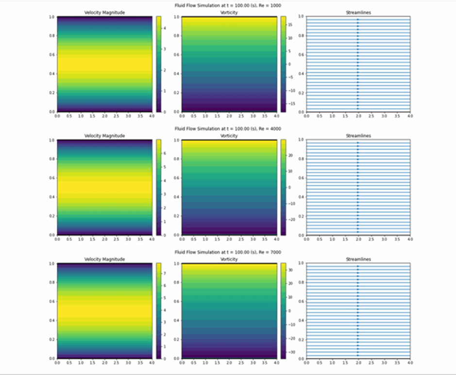
In Figure 1, it visualizes the simulation results at time 100s: the velocity magnitude $|\mathbf{u}| = \sqrt{u_x^2 + u_y^2}$ and vorticity magnitude as color plots and streamline in the rectangular channel.
The Re number is changing from 1,000 to 7,000.
As can be observed, regardless of the Re number, the flows develop a similar profile with the highest velocity at the channel center and smoothly reduce to zero at the wall to satisfy the no-slip condition.
The channel center velocity increases with higher Re number, as higher Re is indicating higher fluid velocity with all other factors remain constant.
The vorticity and streamline plots demonstrate there is nearly no curl of velocity field, and the fluid motion is characterized by smooth and orderly movement of fluid particles in parallel layers, with no mixing between those layers.
The observations are consistent with the Poiseuille’s Law in the ideal case.
Poiseuille’s Law describes the ideal steady-state where the fluid’s time evolution has reached its final state.
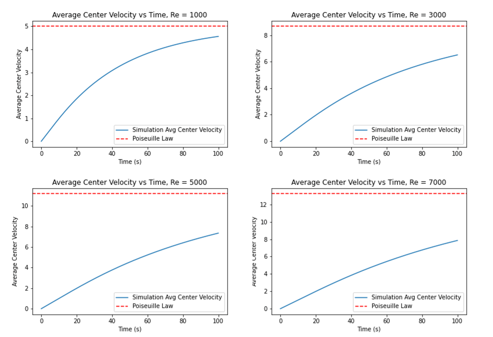
In Figure 2, the simulated center velocity is plotted as a function of time for different Re number, and the dashed line is the theoretical Poiseuille’s Law velocity as a comparison.
It can be observed that the center velocity is approaching to the final Poiseuille’s velocity in all cases but with different approaching rate.
It takes longer time to reach the final steady state for fluid with higher Re number.
This is because the time required for the initial velocity to propagate from the walls to the center is governed by the viscous diffusion timescale, which is approximately $t \sim \frac{L_y^2}{\nu}$ , where $L_y$ is the channel height and $\nu$ is the kinematic viscosity.
At higher $Re \sim \frac{1}{\nu^2}$ , the viscosity $\nu$ is lower, this results in a longer diffusion time for higher Re.
Therefore, approximately it is expected to see $t \sim \frac{L_y^2}{\nu} \sim \frac{L_y^2}{Re}$ .
For example, simulations show velocity reaches ~63% of steady state at 100 seconds at $Re=7,000$ but it takes only ~40 seconds to reach the same velocity at $Re=1,000$ .
Plug in the numbers from simulation, we observe the simulation matches with expectation consistently.

(37) $\begin{equation*}\frac{t_{Re=1,000}}{t_{Re=7,000}} = \frac{40}{100} \sim \frac{L_y^2 / 1,000}{L_y^2 / 7,000} \approx 0.38\end{equation*}$

Figure 2 | Channel Center Velocity as a Function of Simulation Time, Comparing with Poiseuille’s Law

Flow with perturbations

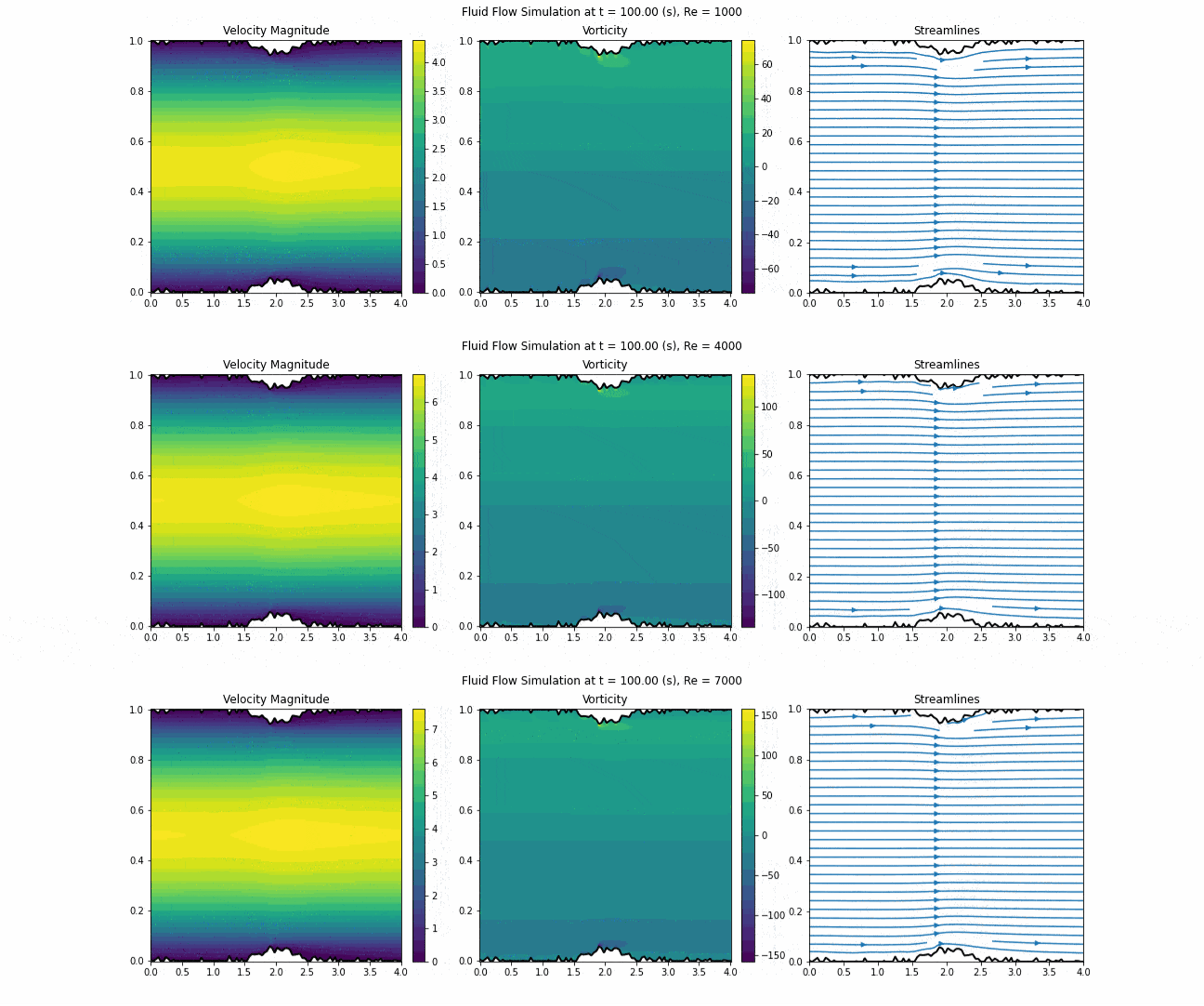
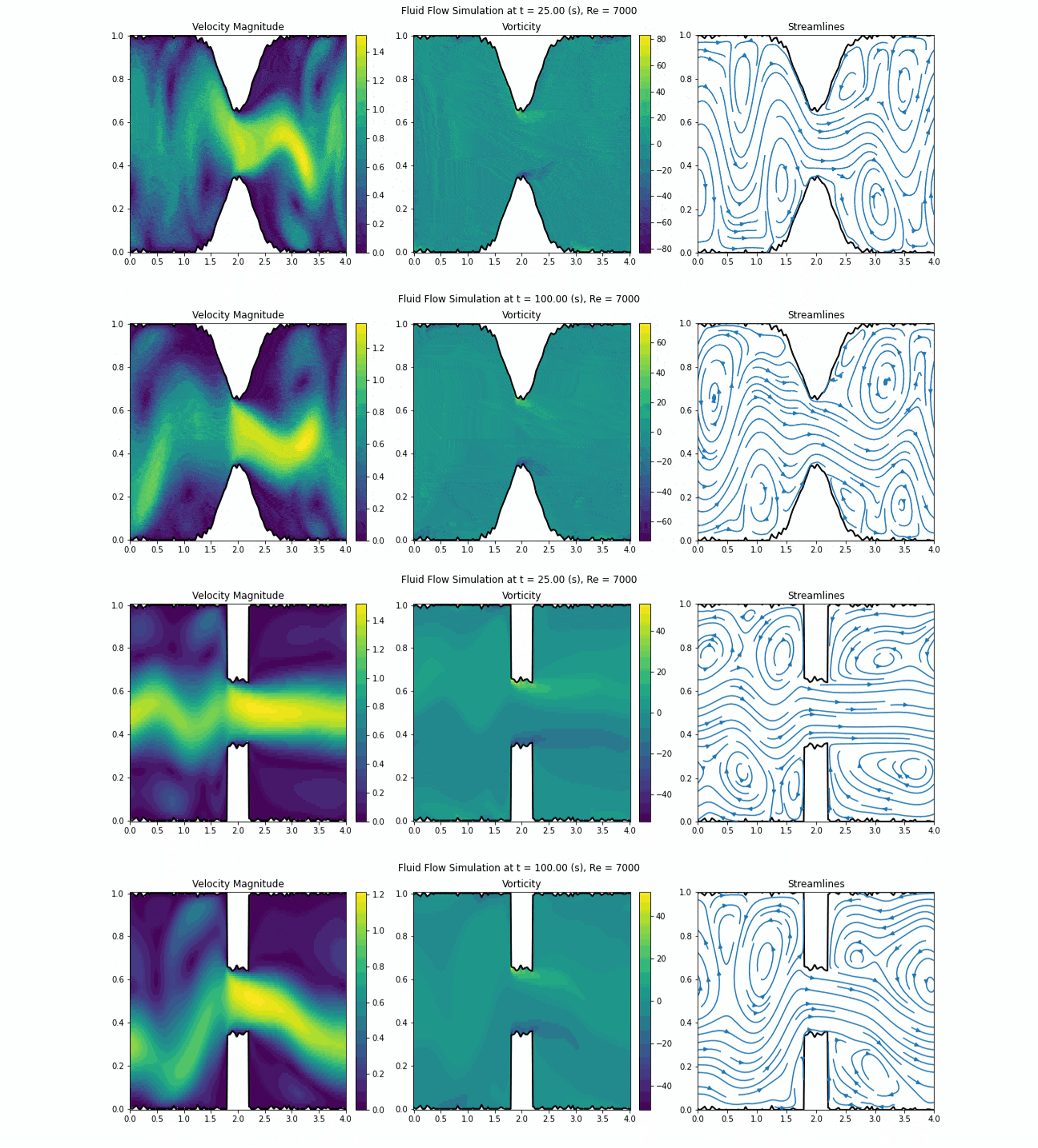
In the next study, we introduce perturbations, i.e. random roughness on the channel wall and different constriction shapes (Gaussian and step-like), to numerically investigate the system with hydraulic resistance, vortex shedding, and viscous energy dissipation in 2D channel flows, for ranging from 1,000 to 7,000. The wall roughness is kept as 1% of the channel half-height and the constriction height increases from 5% to 35% of the channel half-height to simulate different degree of constriction strength. The simulation results at 100s are shown in Figure 3 for Gaussian constriction at 5% strength. It is observed from the streamline plot that the overall flow remains laminar regardless of Re numbers, except that a variation of velocity at the center along the channel direction is induced by the constriction. A higher velocity, ~8%, is observed at the middle of constriction, compared to the leftmost inlet center far away from the middle of constriction. This is because of mass conservation (continuity equation), when the constriction reduces the cross-section area of the channel, the incompressible fluid passes through the narrower region with higher velocity. The vorticity plot shows some small curl of velocity field around the rough wall and constriction as expected.

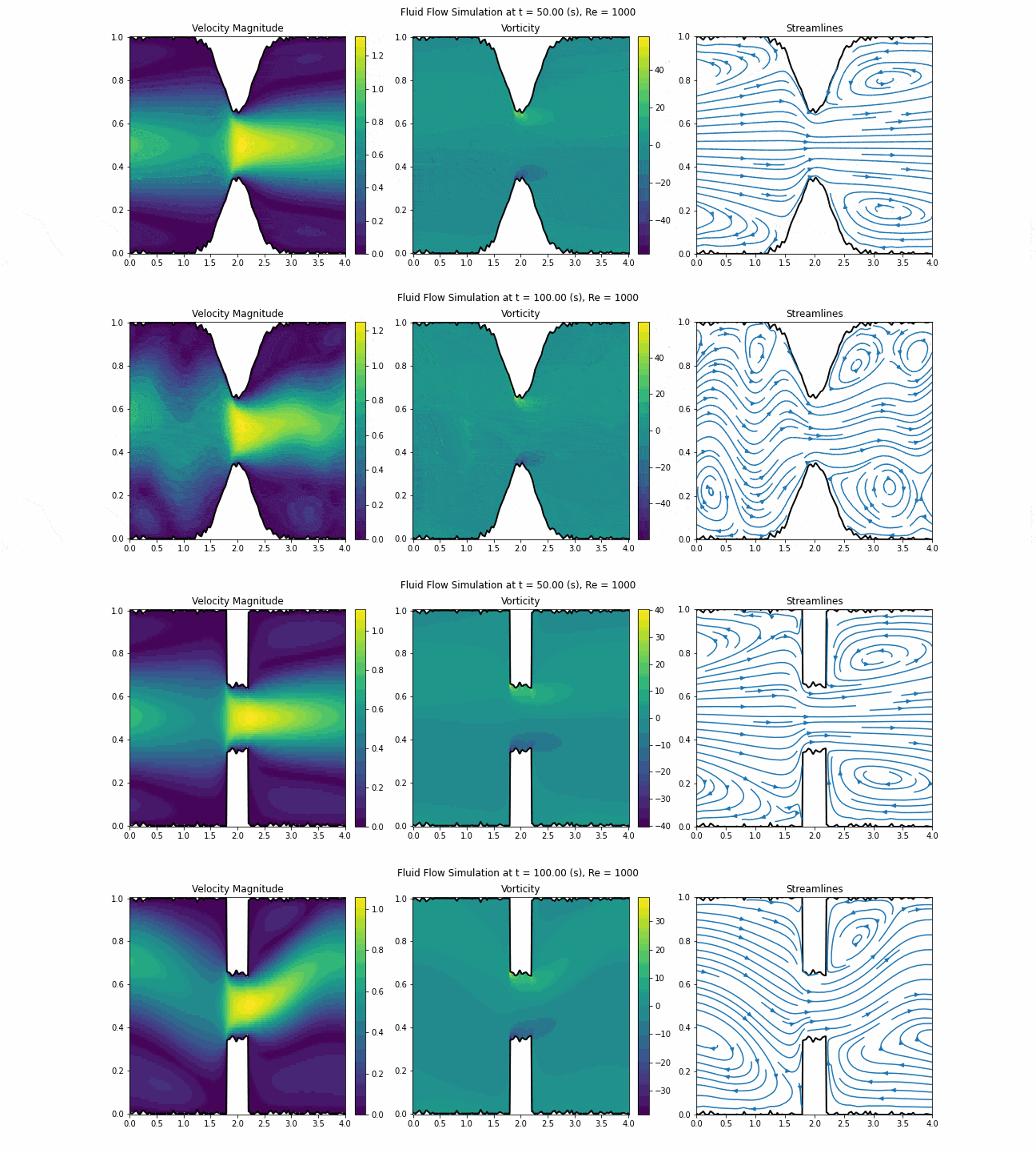
Figure 3 | Fluid Flow at 100s with 5% Gaussian Constriction with Different Re

Now we turn to a more interesting case where the constriction strength is increased to 35% of the channel half-height.
As the simulation results become time dependent, two snapshots at 50s and 100s are shown in Figure 4. At 50s the flow accelerates significantly in the constriction region, indicating a jet-like flow through the narrowing.
Alternating regions of positive and negative vorticity suggest the formation of vortices.
Streamlines converge smoothly into constriction with laminar entry condition. The upstream and downstream show clear recirculation zones due to constriction. At 100s, besides the pronounced high-speed jet flow through the constriction, the velocity and streamline plots show more evident curvature and instability, i.e. vortex shedding, but not fully turbulent with irregular eddies and no periodicity.

If Re is raised to 7,000, significant inertial effect is introduced. As can be seen in Figure 5, periodic vortex shedding and unsteady flow starts to develop as early as 25s and become quasi-periodic at the simulation end time 100s. Compared to Re=1,000 case, stronger jets, larger vortices, and more significant recirculation can be observed.

Figure 4 | Fluid Flow with 35% Gaussian and Step Constriction at 50s and 100s with Re=1,000

To quantify the observations for different simulation cases, we calculate three quantities:
1) Resistance R, defined as the pressure drop normalized by flow rate at the inlet $R = \frac{\Delta p}{Q}$ .
It measures the hydraulic resistance. Higher R indicates greater difficulty for fluid to pass through, typically due to narrower sections, sharper geometries, or flow instabilities. 2) St, Strouhal number, as defined in Section `Nondimensionalization’, f is the shedding frequency measured via FFT on the vorticity time series at a point downstream of the constriction, D is the width of constriction and U is the theoretical Poiseuille velocity at the center. 3) Diss, energy dissipation rate, as defined in Section 2.6. It measures the rate at which kinetic energy is converted to heat due to viscous friction.

Figure 5 | Fluid Flow with 35% Gaussian and Step Constriction at 25s and 100s with Re=7,000

The simulation results are summarized in Table 1 for constriction shape Gaussian and step-like, constriction strength is varied from 5% to 35% and Re is varied from 1,000 to 7,000.
For both Gaussian and step shapes, R increases significantly with strength due to heightened flow obstruction, and generally rises with Re, reflecting inertial losses dominating at higher Re.
Step shapes exhibit slightly higher R than Gaussian, because sharper geometries amplify drag.
St remains low overall (0.0002–0.0349) but shows spikes at high constriction strength/Re for Gaussian and step.
Diss roughly remains flat at low constriction strength and Re for both shapes but increases with higher Re when constriction strength is high.
This is reasonable because, at low constriction strength, the flow remains steady and spatially smooth in the ideal constant-width channel over the Reynolds numbers examined, whereas at high constriction strength, the flow becomes unstable, developing more vortices and shedding, which increases energy dissipation¹⁵^,¹⁶. To provide scale interpretation, we map one of the nondimensional results (5% Gaussian contriction) to a representative vessel diameter $H=3$ mm using blood properties $\rho=1,060$ kg/m³ and $\mu=3.5$ mPa·s, kinematic viscosity $\nu \approx 3.3 \times 10^{-6}$ m²/s.
For $Re=1,000$ , the reference velocity is $U_{ref} = Re , \nu/H$ , giving $U_{ref} \approx 1.1$ m/s.
The dominant unsteadiness is characterized by $St = f D_c / U_{ref}$ with $D_c = H$ , then $f = St , U_{ref} / H$ (e.g., $St = 0.0091 \Rightarrow f \approx 3.3$ Hz at $Re = 1000$ ) and Diss = 1.15, which translates to physical viscous dissipation power $P \approx 4.9$ W/m.
This mapping is provided purely for order-of-magnitude interpretation; because the model is 2D with rigid walls and steady forcing, it does not constitute a predictive hemodynamic model, and higher Reynolds numbers in Table 1 would correspond to either unrealistically high velocities for a 3 mm vessel or to larger vessel diameters.

Constriction Shape	Constriction Strength	Re	R	St	Diss	$\|\nabla \cdot \mathbf{u}\|_2$	$\|\nabla \cdot \mathbf{u}\|_\infty$	$\max \frac{x Q(x) - \bar{Q}}{\bar{Q}}$
Gaussian	5%	1,000	0.84	0.0005	0.10	0.055	3.234	0.04%
Gaussian	5%	4,000	2.93	0.0003	0.08	0.061	4.377	0.06%
Gaussian	5%	7,000	4.43	0.0002	0.07	0.062	4.745	0.07%
Gaussian	35%	1,000	5.32	0.0091	1.15	0.064	3.417	1.09%
Gaussian	35%	4,000	16.30	0.0106	1.91	0.068	4.014	1.08%
Gaussian	35%	7,000	30.53	0.0133	2.14	0.069	4.383	1.09%
Step	5%	1,000	0.95	0.0005	0.08	0.069	4.366	0.07%
Step	5%	4,000	3.69	0.0003	0.07	0.076	4.948	0.09%
Step	5%	7,000	6.52	0.0009	0.07	0.077	5.133	0.09%
Step	35%	1,000	5.76	0.0124	1.14	0.073	4.849	1.99%
Step	35%	4,000	5.55	0.0152	1.06	0.079	7.065	1.63%
Step	35%	7,000	5.96	0.0169	1.86	0.079	6.193	1.78%

Table 1 | Constriction and Re Impact on Fluid Flow

To assess the numerical robustness of the simulations underlying these results, we evaluated several diagnostic and verification metrics.
First, incompressibility enforcement was quantified by computing divergence residuals on the grid over fluid cells: $|\nabla \cdot \mathbf{u}|_2 = \sqrt{\langle(\nabla \cdot \mathbf{u})^2\rangle}$ and $|\nabla \cdot \mathbf{u}|_\infty = \max |\nabla \cdot \mathbf{u}|$ , which tell the typical incompressibility residual level and the worst-case local violation, often near boundaries, respectively.
For a representative case (Re = 1,000, Gaussian constriction, strength 5%), the final-step residuals were $|\nabla \cdot \mathbf{u}|_2 = 5.5 \times 10^{-2}$ and $|\nabla \cdot \mathbf{u}|_\infty = 3.2$ .
This pattern with moderate RMS residuals and larger pointwise maxima, is typical, because $|\cdot|_\infty$ is often dominated by a small number of cells near sharp boundaries or constriction corners.
Mass conservation was independently verified by evaluating the cross-section flow rate $Q(x) = \int u(x,y) \, dy$ along the channel.
For the same case, the maximum relative deviation from the mean was 1.08%, defined as

(38) $\begin{equation*}\max \frac{x Q(x) - \bar{Q}}{\bar{Q}}\end{equation*}$

As can be seen for all the test cases, the incompressibility is preserved, except some local violation around boundaries.
For mass conservation under mild constrictions, this deviation remained $< 0.1\%$ , while for the strongest narrowing (35%) it increased modestly, reaching $\sim 1.1\%$ for Gaussian and up to $\sim 2.0\%$ for step-shaped constrictions.
A time-step refinement study was performed using three time-step sizes ( $\Delta t$ , $\Delta t/2$ , $\Delta t/4$ ) with all other parameters fixed for a representative case (Re = 1,000, Gaussian constriction, strength 5%), and summary metrics were averaged over the last 10 saved time steps at $t_{end} \approx 100$ (short-run diagnostics, see Table 2).
The Strouhal number exhibits excellent convergence, with a relative change of $4 \times 10^{-6}$ between $\Delta t/2$ and $\Delta t/4$ .
The dissipation rate also converges well, with a relative change of approximately $1 \times 10^{-4}$ over the same refinement.
In contrast, the resistance $R = \Delta p / Q$ remains more sensitive to time-step size.
This is expected and not a numerical failure, however, it reflects that the long averaging time is required for pressure-drop statistics in unsteady separated flows.

$\Delta t$	$R_{avg}$	$St_{avg}$	$Diss_{avg}$
0.0005	0.84193	0.00052	0.10396
0.00025	1.67934	0.00052	0.10398
0.000125	3.31223	0.00052	0.10399

Table 2 | Time-step Convergence of Fluid Flow Metrics

Finally, we validated the solver against a canonical benchmark using the 2D Taylor–Green vortex in a periodic box $[0, 2\pi) \times [0, 2\pi)$ with initial condition¹⁷.

(39) $\begin{equation*}u(x,y) = U_0 \sin x \cos y, \quad v(x,y) = -U_0 \cos x \sin y\end{equation*}$

which is analytically divergence-free. For this fundamental mode, the spatially averaged kinetic energy

(40) $\begin{equation*}E(t) = \frac{1}{2}(u^2 + v^2)\end{equation*}$

decays as $E(t) = E_0 e^{-4\nu t}$ . We evolve the flow under periodic boundary conditions using the same numerical structure (semi-Lagrangian advection, viscous diffusion, and projection step for incompressibility), and compare $E_{numerical}(t)$ to the analytical decay law at multiple times, reporting relative errors.
Because semi-Lagrangian advection with bilinear interpolation introduces additional numerical diffusion, agreement with the analytical energy decay is evaluated over short times (t = 0.1s), where the numerical diffusion is negligible compared with physical viscosity.
Over long integration times, the numerical diffusion causes faster-than-physical energy decay, so long-time energy matching is not used as a quantitative benchmark.

Figure 6 | Comparing the Simulated Fully Developed Profile to the Analytical Solution

The relative kinetic-energy error at t=0.1s was 0.04%, confirming correct viscous decay behavior.

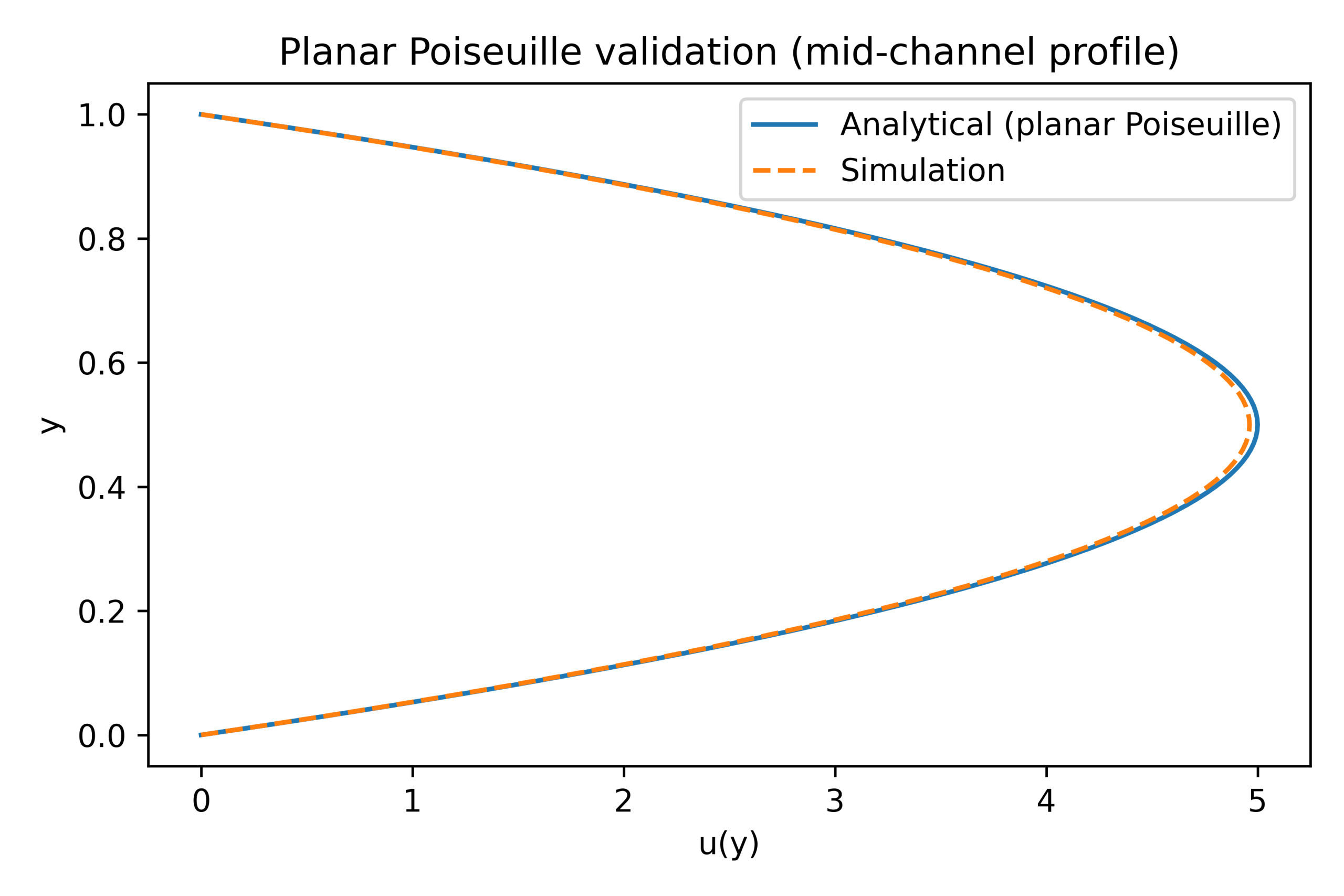
We additionally validated the channel solver against planar Poiseuille flow by comparing the simulated steady velocity profile to the analytical solution (see Figure 6), showing close agreement in the fully developed upstream region.

E_{numerical} — Table 3 | Short-Time Validation of Viscous Decay Using the Taylor–Green Vortex

Particle Deposition in Channel Flow

The fluid flow simulations above reveal how constrictions and Re affect velocity profiles, vorticity, and energy dissipation, real-world applications such as blood flow in vessels or mass transport in pipelines often involve suspended particles that can deposit and cause blockages. To extend the analysis, we now incorporate particles into the channel flow and model their transport, sedimentation, and deposition under gravity, particularly at constrictions. This allows me to investigate clogging dynamics and how flow instabilities influence particle behavior. To simulate realistic scenarios, particles are added to the channel flow where each particle’s motion is governed by Stokes drag from the fluid velocity, gravity-induced sedimentation. The particle motion model assumes Stokes drag, which is formally valid when the particle Reynolds number $Re_p = \rho |\mathbf{u} - \mathbf{u}_p| d_p / \mu \ll 1$ .. Using characteristic velocity differences from the simulations and representative particle sizes, $Re_p$ is expected to remain small at low Reynolds numbers but may approach or exceed unity locally at higher Reynolds numbers (e.g., $Re=7000$ ), particularly near constrictions where velocity gradients are large. In such cases, Stokes drag provides only an approximate description, and higher-order drag corrections would be required for quantitative accuracy. Accordingly, particle-deposition results at high Reynolds numbers should be interpreted qualitatively, as the simplified drag model does not fully capture inertial drag corrections outside the Stokes regime. When a particle intersects a wall or constriction boundary, it is removed from the flow and classified as deposited with a prescribed sticking probability $P_s = 0.2$ . This probabilistic rule is intended as a simplified surrogate for complex adhesion mechanisms and does not represent a calibrated physical sticking law¹⁸. Particles are modeled as passive Lagrangian point particles whose trajectories are integrated in time using an explicit forward-Euler update. At each time step, particle velocities are updated based on the local fluid velocity interpolated from the Eulerian grid using bilinear interpolation. Particle motion includes advection by the flow and a constant gravitational settling term in the wall-normal direction. Hydrodynamic interaction between particles and the fluid is represented using a simplified Stokes-drag approximation, which is valid for small particles at low particle Reynolds number. Particle–particle interactions, finite-size effects, lift forces, lubrication forces near walls, and feedback from particles to the fluid are neglected. As a result, the particle model should be interpreted as a qualitative transport model rather than a quantitative predictor of deposition rates. The simulation sweeps over Re = 1,000 and 7,000, constriction strengths = 5% and 35%, with 1,000 particles. We calculate the clog fraction as No. of stuck particles/total No. of particles. To simulate a continuous flow system, after the particles exits the channel at the right most outlet, they reenter the channel from the left inlet at random positions particle injection locations and wall-collision outcomes are stochastic, the clogging fraction exhibits run-to-run variability. To account for this, reported clogging fractions are interpreted as statistical quantities rather than deterministic outcomes. In this study, the clogging fraction is reported as the mean value over repeated simulations with different random seeds, and variability is characterized using the standard deviation. Trends discussed below are robust relative to this stochastic variability.

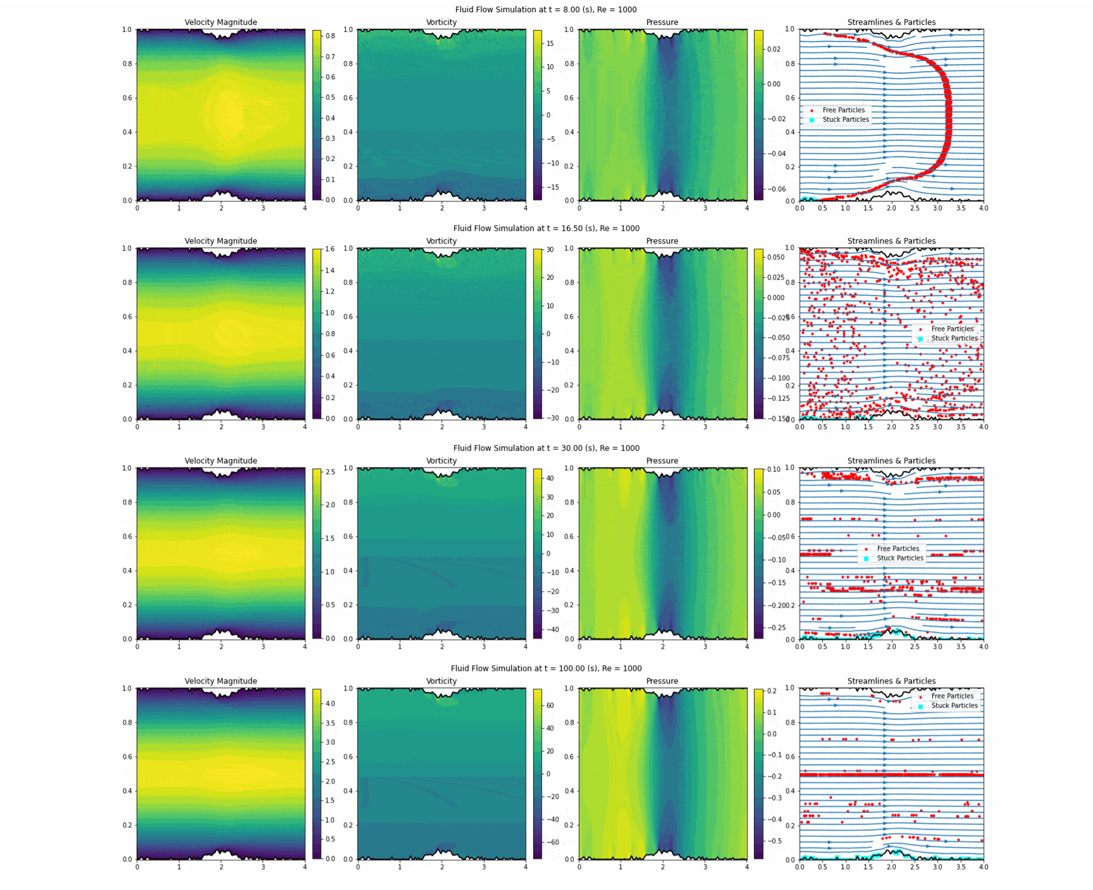
Figure 7 | Particle Transport with Gaussian Constriction at 5% and Re of 1,000 at time 8s, 16.5s, 30s and 100s

Figure 6 shows snapshots of particle positions and trajectories for Re = 1,000 and 5% strength. After 30s of simulation, it illustrates a phenomenon called inertial focusing, where particles align into streamlines near the channel center¹⁹. At moderate Re, inertial forces become significant compared to viscous forces. The nonlinear convective term in the Navier-Stokes equations causes particles to move away from the walls toward regions of lower shear, typically the channel center. often forming single-file lines or focused bands²⁰. While at higher constriction strength of 35% in Figure 7 particles migrate toward walls, depositing near the constriction due to recirculation zones and gravity. At the end of simulation time, there is no inertial focusing that can carry particles through the flow, but significant number of particles deposited at constriction.

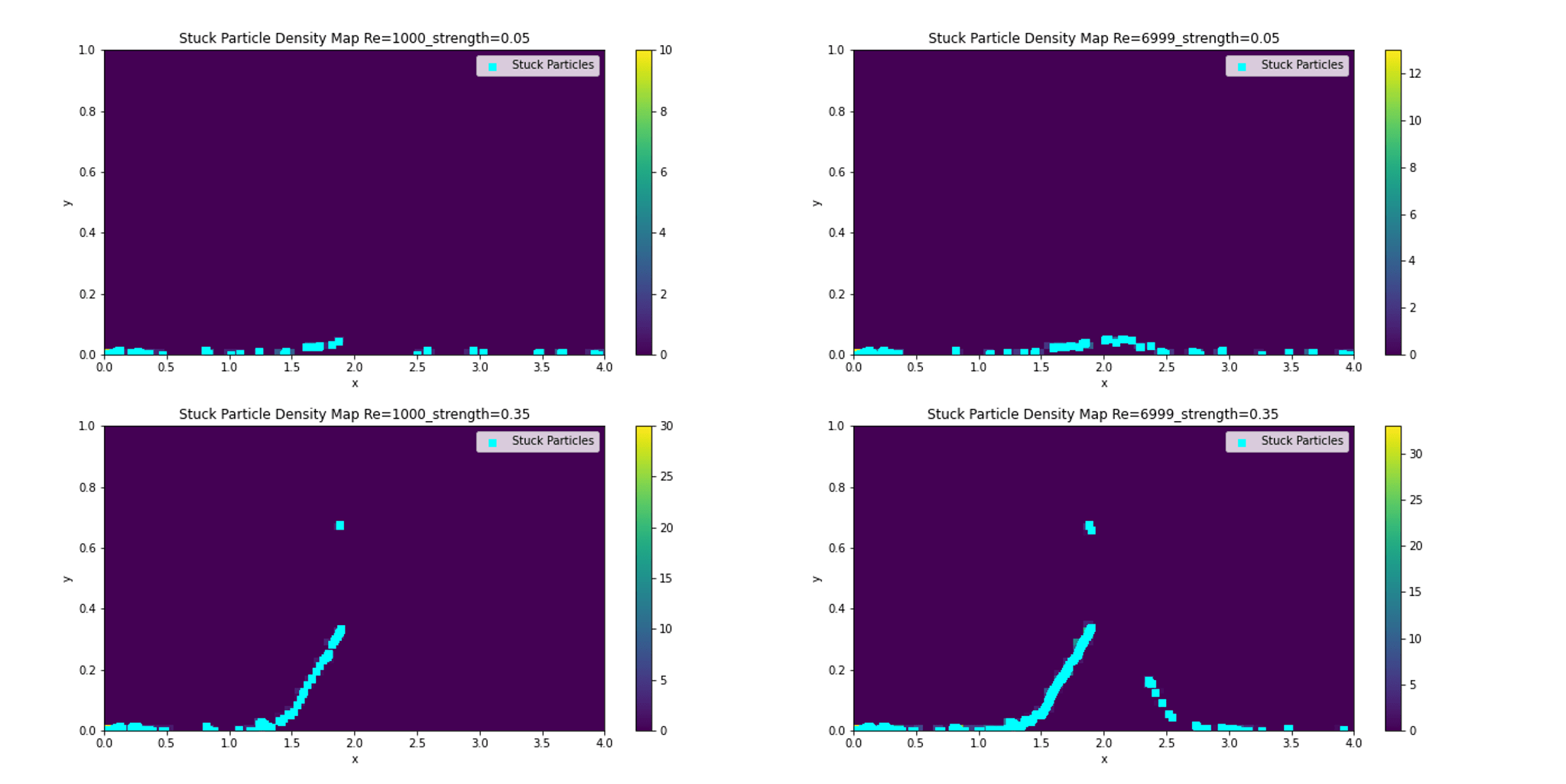
Figure 8 shows the accumulated particles density map at the end of simulation time. The clog fraction increases with Re and strength, from 0.45 at Re=1000, 5% to 0.92 at Re=7000, 35%. The higher inertia amplifies sedimentation and trapping. This aligns with studies on turbulent channel flows, where vortex shedding enhances deposition²¹^,²²^,²³. It effectively narrows the channel, qualitatively illustrating how recirculation-driven deposition can reduce effective flow area in simplified channel flows. One limitation of the study is that it does not consider particle size effect and the probability of particle reentering into flow after deposition. These results still provide insights into the sedimentation or clog formation and help potential for optimizing designs to minimize deposition. The particle-deposition results depend on several modeling parameters, most notably the sticking probability and particle properties such as effective size and density. Increasing the sticking probability would trivially increase the measured clogging fraction, while decreasing it would reduce deposition without altering the underlying flow structures. Similarly, larger or denser particles would experience stronger gravitational settling and enhanced wall encounters, whereas smaller particles would more closely follow fluid streamlines. Although a full parametric sweep is beyond the scope of this study, these dependencies are consistent with established particle-transport theory and do not alter the qualitative conclusion that recirculation zones near constrictions promote increased wall interaction in simplified channel flows.

Figure 9 | Density Map of Particle Deposition of Gaussian Constriction for Different Strength and Re

Discussion

We used numerical simulations to study the dynamics of incompressible fluid flow in channels in a direct and visual manner. At different Reynolds numbers, our solutions successfully reproduced the parabolic velocity profile described by Poiseuille’s law, and the simulations agreed closely with the theoretical analytical solution. To better mimic realistic scenarios, we introduced rough channel walls and localized constrictions. In these cases, we observed that the fluid accelerated through the narrow regions, forming jet-like flows and recirculation zones. This effect was particularly pronounced at higher Reynolds numbers, where inertial forces dominate over viscous dissipation.

To quantify the impact of constriction severity and Reynolds number, we calculated the flow resistance, Strouhal number, and energy dissipation. The results showed that both resistance and energy dissipation increased with stronger constrictions and higher Reynolds numbers. The Strouhal number remained nearly constant at mild constrictions but rose with Reynolds number when the constrictions became severe. At high Reynolds numbers, the hydraulic resistance $R = \Delta p / Q$ depends not only on local dissipation but also on how pressure recovers downstream of the constriction. For sharp step-shaped constrictions, the flow separates abruptly but often reattaches over a relatively short downstream distance, leading to faster pressure recovery. In contrast, smoother Gaussian constrictions can sustain longer shear layers and extended recirculation zones, delaying pressure recovery²⁴^,²⁵. Due to computational limits, the resolution of our simulations was relatively modest, and the simulation times were capped at 100 seconds. With greater computational power in the future, we expect to obtain higher-fidelity results and further insights. Because the simulations are two-dimensional, they cannot capture 3D turbulent transition mechanisms; the observed unsteadiness reflects 2D vortex shedding and separation rather than fully developed turbulence.

We also introduced particles into the flow to investigate transport and deposition patterns under varying constriction geometries and Reynolds numbers, with relevance to phenomena such as arterial blockage or sediment deposition in pipelines. At low Reynolds numbers, we observed inertial focusing, a phenomenon where particles migrate to stable equilibrium positions within the cross-section rather than depositing on the walls. This effect has been observed experimentally in microfluidic channels, blood flow in capillaries, and industrial particle separation systems. At higher Reynolds numbers, deposition increased and became more uniformly distributed along the channel walls. Under strong constrictions, particles accumulated primarily upstream of the narrowing due to the recirculation zones. At even higher Reynolds numbers, irregular flow enhanced particle deposition both upstream and downstream of the constriction, producing a broader and more uniform distribution. Because the particle model neglects finite-size hydrodynamics, particle–particle interactions, wall adhesion physics, and physiological flow conditions, the results should not be interpreted as quantitative predictions of arterial plaque formation or industrial fouling rates, would require substantially more detailed physical modeling and fully three-dimensional, experimentally validated simulations.

All of these studies were carried out in two dimensions. The potential future work can extend the simulations to three dimensions to provide a more realistic picture and capture additional physical mechanisms. Overall, our work demonstrates how the Navier–Stokes equations capture essential features of fluid dynamics in simplified 2D settings and offers qualitative insight into particle transport and deposition mechanisms in confined flows.

References

C.L.M.H. Navier. Mémoire sur les lois du mouvement des fluides. Mémoires de l’Académie Royale des Sciences de l’Institut de France 5, 389–440 (1822). [↩]
G.G. Stokes. On the theories of the internal friction of fluids in motion, and of the equilibrium and motion of elastic solids. Transactions of the Cambridge Philosophical Society 8, 287–305 (1845). [↩]
Clay Mathematics Institute. Navier-Stokes Equation. (2000). [↩]
P. A. Davidson. Turbulence: An Introduction for Scientists and Engineers. Oxford University Press (2015). [↩] [↩]
J.L.M. Poiseuille. Recherches expérimentales sur le mouvement des liquides dans les tubes de très petits diamètres. Comptes Rendus 19, 1164–1171 (1844). [↩]
Ku, D. N. (1997). Blood flow in arteries. Annual Review of Fluid Mechanics, 29, 399–434. (1997). [↩]
J.L.M. Poiseuille. Recherches expérimentales sur le mouvement des liquides dans les tubes de très petits diamètres. Comptes Rendus 19, 1164–1171 (1844). [↩]
F. M. White. Fluid Mechanics. McGraw-Hill Education (2011). [↩]
Williamson, C. H. K., Vortex dynamics in the cylinder wake. Annual Review of Fluid Mechanics, 28, 477–539 (1996). [↩]
Blevins, R. D., Flow-Induced Vibration. Van Nostrand Reinhold (1990). [↩]
A. J. Chorin. Numerical solution of the Navier-Stokes equations. Mathematics of Computation 22(104), 745–762 (1968). [↩]
Temam, R., Sur l’approximation de la solution des équations de Navier–Stokes par la méthode des pas fractionnaires. Archive for Rational Mechanics and Analysis, 33, 377–385. (1969). [↩]
LeVeque, R. J., Finite Difference Methods for Ordinary and Partial Differential Equations: Steady-State and Time-Dependent Problems. Society for Industrial and Applied Mathematics (2007). [↩]
Ferziger, J. H., Perić, M., & Street, R. L. Computational Methods for Fluid Dynamics. Springer, (2020). [↩]
J. P. Matas, J. F. Morris, É. Guazzelli. Inertial migration of rigid spherical particles in Poiseuille flow. Journal of Fluid Mechanics 515, 171–195 (2004). [↩]
D. Di Carlo. Inertial microfluidics. Lab on a Chip 9(21), 3038–3046 (2009). [↩]
Taylor, G. I., & Green, A. E., Mechanism of the production of small eddies from large ones. Proceedings of the Royal Society of London A, 158, 499–521 (1937). [↩]
G. Segre, A. Silberberg. Radial particle displacements in Poiseuille flow of suspensions. Nature 189, 209–210 (1961). [↩]
D. Di Carlo, D. Irimia, R. G. Tompkins, M. Toner. Continuous inertial focusing, ordering, and separation of particles in microchannels. Proceedings of the National Academy of Sciences 104(48), 18892–18897 (2007). [↩]
J. P. Matas, V. Glezer, É. Guazzelli, J. F. Morris. Trains of particles in finite-Reynolds-number pipe flow. Physics of Fluids 16(11), 4192–4195 (2004). [↩]
M. R. Sippola, W. W. Nazaroff. Modeling particle loss in ventilation ducts. Atmospheric Environment 38(36), 6113–6122 (2004). [↩]
C. Marchioli, M. V. Salvetti, A. Soldati. Some issues concerning large-eddy simulation of inertial particle dispersion in turbulent bounded flows. Physics of Fluids 20(4), 040603 (2008). [↩]
Guha, A.,Transport and deposition of particles in turbulent and laminar flow. Annual Review of Fluid Mechanics, 40, 311–341. (2008). [↩]
Pope, S. B., Turbulent Flows. Cambridge University Press. (2000) [↩]
Schlichting, H., & Gersten, K., Boundary-Layer Theory. Springer. (2017). [↩]

t	$E_{numerical}$	$E_{TG}$	Error%
0	0.2500	0.2500	0.00%
0.025	0.2597	0.2499	3.92%
0.05	0.2547	0.2499	1.93%
0.075	0.2517	0.2498	0.77%
0.1	0.2496	0.2498	0.04%

Simulating Incompressible Fluid Flow in a 2D Channel: From Poiseuille’s Law to Realistic Navier-Stokes Solutions

Abstract