A Course Scheduling System Based on an Improved Genetic Algorithm for Complex Scenarios

Abstract

The automated course scheduling problem is a classical NP-complete problem characterized by complex, multi-dimensional constraints arising from real-world teaching scenarios. (NP problems are those for which a proposed solution can be verified quickly (in polynomial time), but for which no efficient (polynomial-time) algorithm to find a solution is currently known.) Traditional enumeration and backtracking algorithms are often inefficient when faced with high constraint densities and complex scheduling requirements such as parallel courses, biweekly alternations, and fixed or consecutive time slots. Unlike many previous scheduling systems that overlooked such special requirements, this work uniquely incorporates support for biweekly alternating courses and parallel courses directly into chromosome adaptation and fitness evaluation, while maintaining extensibility to accommodate emerging scheduling needs. To address these challenges, this paper proposes an improved genetic algorithm (GA) tailored for course scheduling in administrative class-based systems. The algorithm incorporates sequence-based chromosome encoding, a constraint-weighted fitness function, rank-based roulette selection, partially matched crossover (PMX), and an adaptive mutation strategy. Special handling is designed for parallel courses, fixed-time, blocked-time, and consecutive-period courses to ensure solution validity. The system is implemented on a Django-based backend with modular architecture, enabling data configuration, algorithm execution, and result visualization. Experimental validation on real-world high school data—specifically a 12th-grade cohort including 16 teachers, 18 courses, and 3 classes— demonstrates the system’s capability to generate conflict-free schedules efficiently, achieving complete convergence rapidly within a small number of generations. Compared to traditional GAs, the enhanced design significantly improves convergence speed and conflict resolution accuracy, particularly in highly constrained datasets. Results indicate that the proposed GA exhibits strong stability, scalability, and practical applicability, offering a robust solution for complex educational scheduling tasks.

Introduction

Research Background

The automated course scheduling problem is essentially a typical NP-complete problem, with the scheduling process constrained by various factors such as classes, time slots, teachers, classrooms, and so on. Particularly, when considering the specific teaching plans of schools, there are many special scheduling requirements, such as parallel courses that are held at the same time period but attended by different groups of students, biweekly alternating courses, fixed-schedule or non-fixed-schedule courses and others. These requirements cause the complexity of the scheduling problem to grow exponentially. Mathematically, the course scheduling problem is a combinatorial planning problem under multi-dimensional constraints, with teaching plans and various special requirements as the limiting factors. Its essence is to resolve conflicts between various factors. A perfect timetable does not only mean resolving all conflicts, such as hard conflicts where a teacher is assigned to teach multiple classes in the same time period; but also needs to consider the practical operability of the timetable, for example, it needs to address whether the special scheduling requirements mentioned above can be reasonably solved, whether a teacher has to teach multiple courses consecutively in one day, or whether the same course is overly concentrated within a narrow time window, all of which are refered to as soft conflicts. Traditional manual scheduling often requires weeks of time, while automated scheduling can leverage the high-performance computing power of computers to provide optimized and faster solutions. Traditional scheduling algorithms typically use enumeration or backtracking methods. However, they often struggle to deliver acceptable computational efficiency, making them inadequate for real-world applications. Enumeration algorithms require traversing all possible combinations of courses (n), time slots (t), classrooms (r), and teachers (m), which leads to a complexity of ; Backtracking algorithms, while capable of pruning optimization, still often involve a significant amount of ineffective search. For instance, each recursive step tries  possible choices, with a depth of n courses, resulting in a complexity of . Both algorithms have exponential complexity, which can easily lead to long computation times and combinatorial explosion.

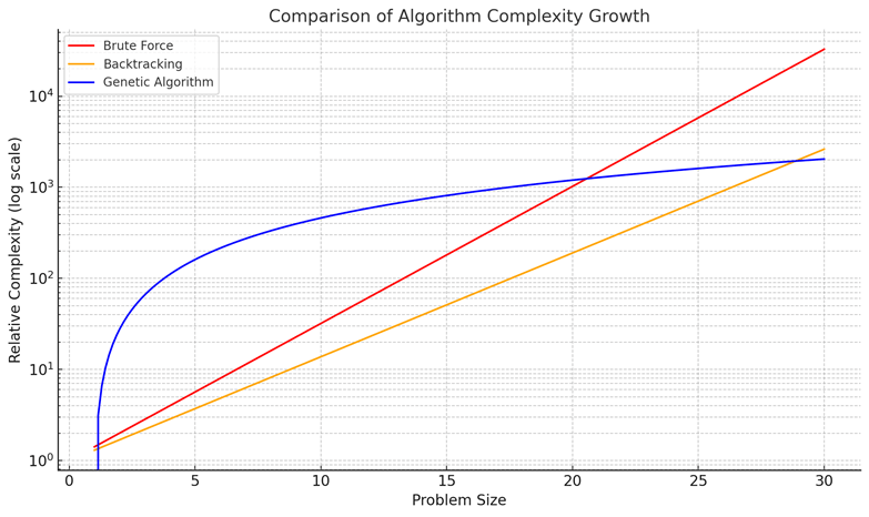
To provide a clearer comparison of algorithmic growth trends, Figure 1 illustrates the relative complexity of enumeration, backtracking, and genetic algorithms as problem size increases. It should be emphasized that this figure is intended for qualitative analysis rather than precise quantitative measurement. The visualization highlights that both enumeration and backtracking methods grow exponentially, quickly becoming computationally infeasible, whereas genetic algorithms, despite initial overhead, exhibit slower growth and maintain better scalability for larger problem sizes.

Heuristic search algorithms are particularly suitable for solving problems with complex solution spaces, such as course scheduling, nurse rostering, and workshop resource allocation. By introducing heuristic information (e.g., domain-specific experience or prior knowledge), these algorithms guide the search process and thus can find approximate solutions close to the global optimum within limited time and hardware resources. Representative algorithms of this class include the Greedy Algorithm, Simulated Annealing, Tabu Search, Particle Swarm Optimization, Ant Colony Optimization, and Genetic Algorithms.

Greedy Algorithm. At each step, the system chooses the currently optimal course arrangement, thereby gradually approaching the global optimum. Papers¹ and² apply the Greedy Algorithm to match students, teachers, and classrooms based on their availability, ensuring that most courses are reasonably scheduled. Paper³ introduces 120 heuristic rules, adopting different course and classroom ordering strategies. However, selecting the best heuristic rule still depends on the specific problem. Essentially, the Greedy Algorithm is based on choosing locally optimal solutions. Although it is simple to implement and runs quickly³, in complex solution spaces it may lead the algorithm to fall into local optima and cannot completely avoid manual intervention.

Simulated Annealing (SA). This algorithm simulates the annealing process in physics, where the key lies in gradually lowering the system temperature to search for the optimal solution. It is suitable for large-scale problems, with a relatively high probability of escaping local optima and converging to the global optimum⁴. However, it is sensitive to parameters such as the initial temperature and cooling rate, which need to be reasonably tuned during the algorithm process⁵. Moreover, due to its probabilistic nature, simulated annealing may not handle soft constraints (such as teacher preferences or classroom utilization) effectively, requiring further optimization of the fitness function⁶.

Tabu Search. As a heuristic algorithm based on local search, it continuously explores the neighborhood of the current solution to seek the optimum. Its core idea is to maintain a Tabu List that records previously visited solutions or executed operations, thus preventing the search from revisiting already explored solutions and avoiding entrapment in local optima^7,8. The performance of Tabu Search largely depends on parameter settings such as the size of the Tabu List, tabu tenure, neighborhood definition, and stopping criteria. Although Paper⁹uses adaptive mechanisms for parameter tuning, further improvements are still needed to reduce dependence on specific parameter settings.

Particle Swarm Optimization (PSO) and Ant Colony Optimization (ACO). Both algorithms are inspired by the behavior of biological systems in nature. PSO simulates the foraging behavior of bird flocks, where each bird is regarded as a particle. Particles share information, and each particle adjusts its position and velocity based on individual and group experiences. Papers¹⁰and¹¹validate PSO using real datasets from middle schools and universities, achieving strong performance, though its effectiveness may decline under more complex and fine-grained constraints. Paper¹²applies PSO to schedule thesis defenses, generating feasible timetables within a reasonable time, but its suitability for more complex scheduling scenarios remains uncertain. ACO, on the other hand, simulates ants’ food-foraging process, where each ant chooses paths based on pheromone concentrations left by previous ants, while also depositing pheromones to influence subsequent ants’ choices. Paper¹³applies ACO to university lab scheduling, while Paper¹⁴and¹⁵apply it to exam scheduling. These works achieved good results and were put into practice, but it is still unclear whether the method is effective in other more complex scheduling scenarios.

Genetic Algorithm (GA) is a heuristic optimization algorithm that simulates the natural selection mechanism in biological evolution. It is particularly suitable for solving NP-complete combinatorial optimization problems like course scheduling. Compared to traditional enumeration or backtracking algorithms, it has the following significant advantages in scheduling: it performs directed searches in high-dimensional solution spaces, utilizes fitness functions to handle various constraints, and, and obtains the optimal solution within a limited timeframe by evaluating either the fitness threshold or the number of evolutionary iterations. However, traditional genetic algorithms, when dealing with real-world scenarios that have high constraint densities, face two major challenges: they tend to converge slowly and are prone to being trapped in local optima, while also being difficult to meet special teaching requirements, such as teachers’ preferences and special teaching requirements^16,17. Therefore, this paper proposes an improved genetic algorithm to better adapt to complex scheduling requirements in complicated scenarios. This algorithm is suitable for scheduling courses based on administrative classes, but not for individualized or elective-based models (e.g., modular or flexible grouping). Hence, classroom resources are not considered a constraint in this scheduling system, as classrooms for most administrative classes are fixed.

Definition of Terms

The following are explanations for some special scheduling constraints in the teaching scenario:

• Parallel Courses: Different students within the same class take different courses during the same time slot.
• Biweek alternating Courses: For the same class and time slot, two courses alternate between odd and even weeks.
• Fixed/Blocked Time Slot Courses: Courses need to be scheduled during a specified time slot, or they cannot be scheduled during a specified time slot.
• Consecutive Period Courses: According to the teaching plan, certain courses need to be scheduled consecutively. For example, Course A is taught 6 times a week, but requires two consecutive periods, which will be completed in three sessions.

Methods

Algorithm Workflow

• Obtain course configuration data;
• Based on the course configuration, randomly generate multiple timetable chromosomes to form the initial population;
• Evaluate the fitness of each timetable chromosome by calculating the weighted sum of conflicts;
• Use a rank-based roulette wheel selection to select high-quality chromosomes;
• Perform crossover and mutation operations on the selected high-quality chromosomes;
• Repeat steps 3–5 until the fitness meets the required threshold or the maximum number of generations is reached.

Chromosome Encoding

In genetic algorithms, chromosome encoding determines the feasibility and convergence speed of the algorithm. Common encoding methods include sequence encoding, binary encoding, and real-number encoding. Considering that scheduling resources (such as courses, teachers, classes, etc.) are limited discrete values and mutually exclusive with an inherent order, this system adopts sequence encoding for the chromosome to ensure the legality of the timetable.

It is worth noting that in the first step of the algorithm—obtaining the course configuration—the mapping between teachers, classes and courses is manually specified. This means that teacher teaches which course to which class is predetermined based on the school’s teaching plan. The same teacher can teach different classes or different courses, and the same course in different classes can be taught by different teachers. In chromosome encoding, each possible timetable is represented as a chromosome, where each gene corresponds to a course instance. It should be noted that a “course instance” here refers to a specific course uniquely determined by the combination of a class and a teacher. For example, Teacher A teaching Course C to Class 1 and Teacher B teaching Course C to Class 2 are different genes in the chromosome, even though they both teach Course C, because the teacher and class differ. If a course instance has n periods in a week, then this course instance will appear n times in the chromosome. Therefore, a gene can be represented by the expression:

   

where i,j,k, represent j-th time period on the i-th school day of the week for class k; m represents the m-th course in the course set; and n represents the n-th occurrence of course m for class k in that week. The chromosome is a one-dimensional array, with each gene arranged in the order of “day – period – class”. Suppose that the school days are Monday to Friday（i (1-5)）, with seven periods per day (j (1-7)), and three classes for one grade (k (1-3)), courses m are randomly selected from the course set and filled into the array following the order (i,j,k). Meanwhile, n keeps track of how many times course m has been scheduled for class k during the week. This results in a chromosome similar to:

   

where represents Class 1 is assgined the first occurrence of Course 1 in the first period on Monday, and represents Class 3 is assigned the second occurrence of Course 4 in the seventh period on Monday, the same structure applies to the rest of the timetable.

The total length of the chromosome is given by the product of the number of school days (I), the number of class periods per day (J), and the number of classes (K), that is, I × J × K. This reflects the total number of time slots that need to be assigned across all classes within a week.

When generating the timetable chromosome, in order to speed up convergence, avoid unnecessary conflicts, and improve the quality of feasible solutions, constraints must be applied when inserting genes into the chromosome based on special teaching requirements. The strategies that can be considered are as follows:

   

which indicates that the first occurrence of Course 1 and Course 2 for Class 1 are scheduled in the first period on Monday. Biweek alternating courses can also be represented as a gene combination that occupies only a single gene position. Regardless of whether it is the odd or even week, the same position in the chromosome must be assigned a course that is conflict-free with respect to other scheduled courses. In practice, these types of courses are stored in a sequence data structure, where multiple courses are treated as a single element. During fitness evaluation, the algorithm iterates each course through the array to compute conflicts and penalties accordingly.

1. For Fixed/Blocked time slot courses, these courses can be sequentially arranged into specified time slots based on settings, or they can be avoided and inserted into other available time slots in the chromosome.
   – For consecutive period courses, they can be assigned to adjacent gene positions based on the number of consecutive sessions specified in the course configuration. However, care must be taken to avoid situations where consecutive courses cannot be scheduled due to the time slots being too late in the morning or afternoon.
2. To ensure the feasibility of the timetable, course instances inserted into the chromosome need to be randomly selected with a uniform probability to achieve a balanced distribution. However, perfect balance is not necessary, as the fitness function incorporates a penalty for uneven course distribution, allowing the evolutionary process to iteratively refine the timetable toward a more optimal configuration.

Fitness Calculation

In genetic algorithms, fitness and the evolutionary process have a “two-way driving” relationship. The fitness function guides the evolution direction of the genetic algorithm, while the evolutionary process continuously optimizes the fitness function through population evolution and iteration. The fitness function in this algorithm aims to evaluate the degree to which each chromosome (i.e., timetable) satisfies the constraint conditions. The fitness function is calculated as the cumulative penalty for constraint violations, considering both the frequency and the severity of violations. The fitness function is as follows:

   

Where,

• ​ represents the fitness of the i-th chromosome;
• Req_k represents the fitness of the k-th constraint;
• n represents the total number of constraints to be checked
• ​ represents the penalty weight for the k-th constraint;
• T_k represents the number of times the k-th conflict occurs.

The constraints are divided into two levels:

• Primary constraints (also called hard constraints) are the essential ones that must be satisfied. If any primary constraint is violated, the chromosome (timetable) is considered invalid.
• Secondary constraints (also called soft constraints) are applied after the primary constraints are satisfied, aiming to adjust the timetable to make it more practically feasible. The weight for primary constraints is typically larger than that for secondary constraints.

The penalty weights are deliberately set with different magnitudes to distinguish between hard and soft constraints. Higher weights (typically between 8–12, such as 10 for Constraint 1) are assigned to hard constraints that must be satisfied, ensuring they are prioritized during early convergence. Lower weights (ranging from 0.1–1, such as 0.1 for Constraint 4) are used for soft constraints, which allows the algorithm to fine-tune solutions in later iterations without overwhelming the search process. This scale differentiation accelerates convergence by strongly penalizing infeasible schedules first, and then gradually optimizing toward more balanced and practical timetables.

Based on the teaching requirements, this system defines five constraints, each with its definition and penalty calculation method as follows:

Constraint 1: Teacher Schedule Conflicts
A teacher cannot teach different classes at the same time period. This constraint also applies to parallel courses and biweek alternating courses. The penalty weight for each conflict is 10.

Constraint 2: Teachers with Special Time Slot Requirements
Teachers with specific time slot requirements cannot be scheduled on certain school days or during specified time slots. The penalty weight for each conflict is 1.

Constraint 3: Maximum Period Number of a Course per Day for a Class
A class cannot have more than three periods of the same course on the same day, unless the user explicitly configures the course to require consecutive periods exceeding three, in which case no penalty is applied. The penalty weight for each conflict is 0.3.

Constraint 4: Teacher’s Consecutive Periods on the Same Day
A teacher cannot teach too many consecutive peroids on the same day, e.g., no more than four consecutive periods, even if they are different courses . The penalty weight for each conflict is 0.1.

Constraint 5: Course Distribution Balance for Each Class
The courses for each class should be evenly distributed throughout the week. The balance coefficient for each course instance is calculated using the following formula:calculated using the following formula:

   

Where，

• ​ represents the balance coefficient for the k-th course instance.
• MaxDay represents the number of days required for the most balanced distribution. If the number of periods for the course instance exceeds the number of school days in the week, MaxDay equals the number of school days; otherwise, it equals the number of periods. ActualDay represents the actual number of school days occupied by the course instance in the chromosome.
• The value 1 in the denominator represents the number of days occupied under the most unbalanced distribution, where the course instances are all scheduled on the same day.
• W is the weight coefficient, set to 0.1.

Example: Suppose a course has 3 periods per week and the school week has 5 days. In the most balanced case, the 3 periods should be spread across 3 separate days, so MaxDay=3. If in a given schedule these 3 periods are only arranged across 2 days, then ActualDay =2. Substituting into the formula gives:

   

This reflects a partial imbalance, since the course is not fully spread across the available days.

The sum of the balance coefficients for all course instances is:

   

Where M is the total number of course instances.

From the fitness function perspective, the smaller the fitness value, the fewer the conflicts or the lighter their severity. Primary constraints must be fully satisfied (e.g., Constraints 1 and 2); otherwise, the chromosome will be considered a poor gene and will gradually be eliminated. Soft conflicts should be minimized as much as possible. If the fitness is less than or equal to the specified minimum fitness, the chromosome is considered a high-quality gene, potentially even the optimal solution.

Population Iteration

In genetic algorithms, common population models include the Steady-State Model and the Generational Model¹⁸. The Generational Model refers to replacing the entire parent population with offspring during each generation. This approach may result in the loss of high-fitness chromosomes from the parent generation, or in the offspring having worse fitness than their parents, leading to oscillations during the evolutionary process.

In this system, the Steady-State Model is adopted for population iteration. Specifically, a new generation of offspring with the same population size as the parent generation is generated. Then, all individuals (both parents and offspring) are sorted based on their fitness. To maintain a fixed population size, the top-performing chromosomes are retained to form the new population, while the bottom half of the lower-quality chromosomes are eliminated. In the course scheduling context, retaining high-quality individuals is particularly important because feasible timetables that satisfy hard constraints (e.g., avoiding teacher or classroom conflicts) may be rare, and once such solutions appear, losing them could significantly delay or even prevent convergence to a valid schedule. This ensures a continuous optimization trend for the entire population and avoids falling into local optima.

Crossover Operation

The crossover of chromosomes ensures that the genetic algorithm can continuously generate new offspring individuals.

First, it is essential to select suitable parent chromosomes to produce offspring. Common selection methods include roulette wheel selection, rank-based roulette selection, elitist selection, and tournament selection¹⁹. Since the fitness differences between chromosomes can be significant, traditional roulette wheel selection tends to overemphasize a few individuals with the best fitness, which can reduce population diversity and ultimately affect the quality of evolution. To address this, the system adopts the rank-based roulette selection strategy:
     Chromosomes are first ranked based on their fitness values, and then selection probabilities are assigned proportionally based on their ranks, which enhances both the stability and diversity of the selection process.

Since course chromosomes use sequential encoding, crossover operations must ensure that the resulting chromosomes do not lose or duplicate any genes. This requires relatively complex calculations. The system adopts the Partially Matched Crossover (PMX) approach²⁰. PMX is particularly suitable here because it is designed for sequence-based representations, ensuring that the sequential structure of timetable chromosomes is preserved while maintaining gene validity. PMX works by randomly selecting two crossover points to define a crossover region. A mapping relationship is then established within this region between the chromosomes of each parent to correct for any repeated genes and ensure gene validity. The detailed process is illustrated in Figure 2:

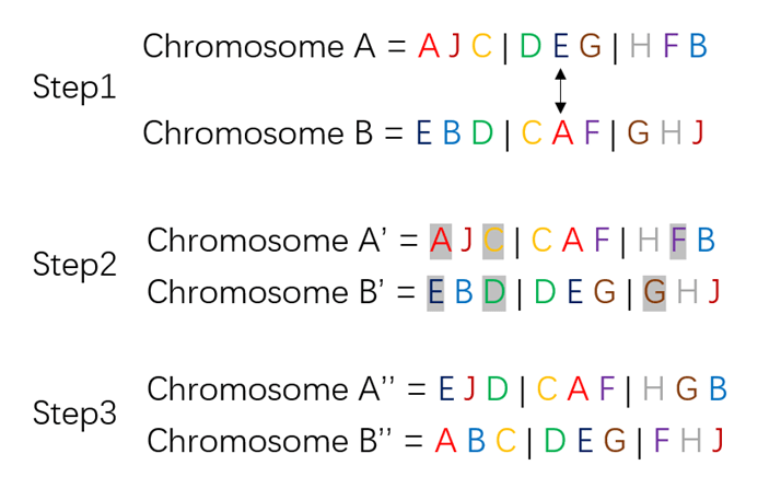
As shown in Figure 2, Step 1 selects two crossover points and swaps the corresponding segments; Step 2 establishes the mapping relationship and corrects duplicate genes; Step 3 produces the final valid offspring chromosomes. This ensures that each gene appears exactly once while maintaining the sequential structure of the chromosome.

Special handling is required for special types of courses during crossover:

• Fixed time-slot courses retain their fixed positions during crossover and do not participate in crossover operations to maintain chromosome validity.
• Blocked time slot course must be carefully checked after crossover to ensure their assigned positions do not fall within any forbidden time slots.
• Consecutive period courses must be treated as a whole during crossover to maintain continuity and prevent scheduling across non-consecutive time slots.

Mutation Operation

In this system, the mutation probability is determined by an adaptive probability based on individual fitness²¹. The specific fitness-based function is as follows:

   

Where:

•  is the mutation probability of the current gene;
• is the minimum mutation probability, set to 0.1;
• ​ is the maximum mutation probability, set to 0.5;
•  is the fitness of the i-th chromosome;
• ​ is the average fitness of the population;
• ​ is the best fitness in the population.

This formula indicates that for low-quality individuals (i.e., those with fitness worse than the population average), the mutation should be carried out with the maximum probability to enhance exploration ability and avoid falling into local optima. For high-quality individuals (i.e., those with fitness better than the population average), the mutation probability should be reduced to preserve advantageous genes.

The value =0.1 and =0.5​ are set empirically. A maximum of 0.5 provides sufficient exploration without excessively disrupting chromosome structures, while a minimum of 0.1 maintains a baseline of randomness to prevent premature convergence.

     The mutation operation is performed by randomly selecting two courses within a chromosome marked for mutation and swapping their positions. To ensure the validity of the result chromosome, special handling is applied for special courses. During mutation, courses scheduled in fixed time slots are excluded — their positions remain unchanged throughout the evolution and do not participate in the swap operation. Blocked time slot courses must not be swapped into these restricted periods. Consecutive period courses should be treated as indivisible units during mutation to prevent their continuity from being disrupted..

System Architecture

The backend of this system is developed using the Django framework, and its overall architecture is composed of four functional applications (Apps), each responsible for a different subsystem task:

Presets (Preset Processing App): Responsible for parsing scheduling data imported by users (such as teacher information, course information, etc.), performing legality checks, and converting the data into structured formats.

Projects (Project Management App): Enables users to create and manage scheduling projects, including managing basic project information (such as classes, grades, etc.), maintaining project status, and performing project edits.

Scheduler (Scheduling Execution App): Handles the invocation of the scheduling algorithm and manages each scheduling task and its results.

Users (User Management App): Provides user registration, login, and permission management functionalities, supporting concurrent access by multiple users.

     The system uses a modular design to achieve logical separation and functional independence, which facilitates future maintenance and scalability. Additionally, Django’s built-in ORM (Object-Relational Mapping) mechanism is employed to manage data models, eliminating the need to manually write SQL statements and reducing redundancy. The data models of each functional module are defined using Python classes and automatically mapped to relational database tables via ORM. This results in tight integration between business logic and database operations. In practice, the use of ORM allows the project to manage data models through object structure editing, thus saving development time.

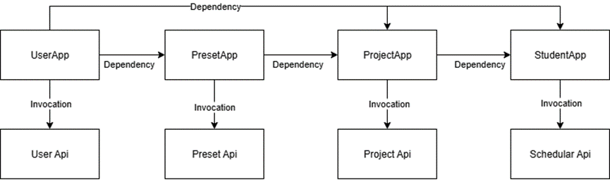
Figure 3 illustrates the invocation relationships among the application modules of the system. The arrows in the diagram represent the dependency and invocation relationships between modules. For example, the ProjectApp depends on user data from the UserApp and preset information from the PresetApp to complete user binding and preset loading when creating a scheduling project. Similarly, the SchedulerApp calls data from the ProjectApp to execute specific scheduling tasks.

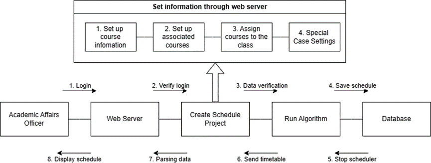
The system’s operational workflow follows a three-tier logic structure of “Data Configuration – Algorithm Execution – Result Visualization” (as shown in Figure 4).

     In the data configuration phase, academic staff complete multi-step setups across several pages, including course-to-class associations, class allocations, and the marking of unavailable time slots for teachers. After validation by the Presets module, the data is passed to the Scheduler module, which invokes the improved genetic algorithm to generate a conflict-free timetable. The final results are then distributed based on user role permissions — for example, students can only view their own class schedule, and teachers can only view their own teaching assignments.

     The system defines four user roles to meet the operational needs and permission levels of different user types:

1. Super Administrator: Holds the highest level of system privileges, responsible for overall platform management, including system-level operations such as the creation and modification of academic staff accounts.
2. Academic Staff (Schedulers): Have full control over scheduling functions. They can create and edit timetables, run scheduling tasks, and publish results. They are also responsible for creating and managing teacher and student accounts.
3. Teachers: Have restricted access and can only view schedule information related to their own courses.
4. Students: Can view their own class timetables to check their personal course arrangements.

     The hierarchical permission structure significantly enhances system maintainability and scalability, especially as the number of users or the complexity of scheduling grows. Super administrators focus only on top-level configurations and global academic account management, rather than being burdened with managing every user directly. Instead, lower-level administrators and academic staff are empowered to handle routine scheduling tasks, user account operations, and day-to-day adjustments. By restricting teachers and students to only the information and functions relevant to them, the design avoids permission clutter, preserves clarity, and maintains both operational efficiency and a positive user experience.

Result and discussion

This system selects a 12th-grade cohort from the Senior High School Division of a typical urban high school as the test case. The selected division includes 16 teachers, 18 different courses, and 3 classes.

Experimental Results

Figure 5 shows the class timetable generated by the system.

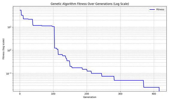
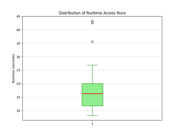
Figure 6 shows the relationship between the number of evolutionary generations and the fitness value. It can be observed that the fitness value decreases as the number of generations increases. Around the 417th generation, the fitness value reaches 0, indicating that all hard constraints—such as no course conflicts and no violations of special scheduling requirements—are satisfied. At the same time, soft constraints like continuous teaching for teachers and unbalanced course distribution are also resolved. The total execution time of the program on a standard notebook environment (Intel i7-10875H CPU, 16 GB RAM) is 19.8699 seconds. To further evaluate the efficiency of the algorithm, Figure 9 shows the distribution of runtime across 30 independent runs. The average runtime is 18.29 ± 8.87 seconds, indicating that most runs complete within a practical time budget, with only a few outliers.

Analysis

From Figure 6, it can be seen that the fitness value of the genetic algorithm decreases most significantly within the first 100 generations. This indicates that the algorithm exhibits strong global search capabilities in the early stages, quickly identifying and preserving high-quality individuals. In particular, the fitness drops sharply in a step-like pattern during the first 50 generations, suggesting that high-quality solutions are rapidly optimized at the beginning, and most hard conflicts with higher weights are effectively resolved early on.

As the number of generations increases, the rate of fitness improvement gradually slows down. After around the 150th generation, the algorithm enters a convergence phase, with the fitness changes stabilizing. This reflects the algorithm’s shift from global search to localized fine-tuning. At this stage, population diversity decreases, and mutation and selection operations mainly focus on slight improvements around existing high-quality individuals. The emphasis shifts to resolving soft constraints, resulting in a slower convergence pace. This fast-then-slow convergence pattern can also serve a practical role: in the early stage, the algorithm provides users with a preliminary acceptable solution range and an expectation of the final outcome. If the expected solution fails to resolve primaryconflict (hard conflict), the system can prompt users to review and adjust their data settings.

Overall, the genetic algorithm implemented in this system achieves effective convergence within approximately 400 generations. The final fitness value reaches 0, confirming the effectiveness of the designed selection, crossover, and mutation strategies for this specific problem.

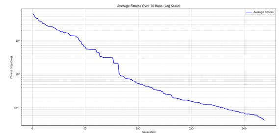
Figure 7 shows the average fitness decline trend over multiple independent runs. Despite differences in the initial populations and search paths of each run, the overall trend remains highly consistent. The average curve also shows a clear “fast-then-slow” convergence pattern. While not every run reaches a fitness value of 0, all hard constraints are successfully resolved (as each hard conflict carries a penalty weight of 1 or greater). In some runs, the final fitness falls between 0.015 and 0.025, indicating that a small number of courses are slightly unbalanced in distribution, but still yield acceptable and usable schedules.

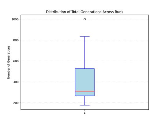
Figure 8 presents the distribution of the total number of generations required for convergence across 30 runs. On average, convergence is achieved within 414.27 ± 217.15 generations, with the majority of runs stabilizing before the 500th generation.

Under a fixed computational budget, the algorithm achieves an average final fitness of 0.0016, with a success rate of 93.3% in reaching a fitness value of 0. These results demonstrate that the algorithm has strong stability and robustness.

Repeated runs consistently optimize the solution space effectively, further verifying the reliability and practicality of the algorithm in solving the scheduling problem.

Conclusion

In summary, this system is designed and implemented to address complex course scheduling scenarios using an improved genetic algorithm. By incorporating a rank-based roulette wheel selection strategy, partially matched crossover mechanism, constraint-driven fitness function, and an adaptive mutation method, the system demonstrates strong convergence and practical applicability when tested on real teaching data.

Experimental results show that the system can quickly generate conflict-free schedules that satisfy various special scheduling requirements. In real-world educational administration, this significantly improves the efficiency of scheduling tasks and provides greater flexibility in handling special constraints and personalized teaching requirements. Since this study focuses on class-based scheduling, each administrative class is assumed to have a fixed classroom. There is limited demand for additional classrooms. Thus the system does not address additional classroom allocation for elective or cross-class courses. In future work, the system could be extended to support elective course models, where student satisfaction rates are incorporated into the genetic fitness function as an additional evaluation factor.

References

1. J. Xiao，The application of greedy algorithm in the course selection and scheduling system of college students, Applied and Computational Engineering, Vol. 75, pp. 48-53 (2024). [↩]
2. J. B. C. Legaspi, R. M. D. Angel, A. Lagman, J. H. J. Ortega，Web Based Course Scheduling System Using Greedy Algorithm，International Journal of Simulation: Systems, Science & Technology, Vol. 20, No. S2, pp.14.1-14.7 (2019). [↩]
3. B. M. Coşar, B. Say, T. Dökeroğlu，A New Greedy Algorithm for the Curriculum-based Course Timetabling Problem，Düzce University Journal of Science and Technology, Vol. 11, Issue 2, pp. 1121-1136 (2023). [↩] [↩]
4. J.Frausto-Solís, F. Alonso-Pecina, J.Mora-Vargas, An Efficient Simulated Annealing Algorithm for Feasible Solutions of Course Timetabling. MICAI 2008: Advances in Artificial Intelligence, Vol. 5317, pp. 675–685 (2008). [↩]
5. C. Akkan, A. Gülcü, Z. Kuş, Bi-criteria Simulated Annealing for the Curriculum-Based Course Timetabling Problem with Robustness Approximation, Journal of Scheduling, Vol. 25(4), 477–501 (2022). [↩]
6. N. Basir, W. Ismail, N. M. Norwawi, A Simulated Annealing for Tahmidi Course Timetabling, Procedia Technology, Vol.11, pp. 437-445 (2013). [↩]
7. Z. Lü, J. Hao, Adaptive Tabu Search for course timetabling, European Journal of Operational Research, Vol 200 (1), pp. 235-244 (2010). [↩]
8. A. R. Mushi, Tabu Search Heuristic For University Course Timetabling Problem, African Journal of Science and Technology (AJST) Science and Engineering Series, Vol. 7(1), pp. 34-40 (2006). [↩]
9. S. Hooshmand, M. Behshameh, O. Hamidi, A tabu search algorithm with efficient diversification strategy for high school timetabling problem, International Journal of Computer Science & Information Technology (IJCSIT),Vol 5(4), pp. 21-34 (2013). [↩]
10. I. X. Tassopoulos, G. N. Beligiannis，Using particle swarm optimization to solve effectively the school timetabling problem, Soft Computing, Vol.16, pp.1229–1252 (2012). [↩]
11. I. S. F. Ho, S. Deris, S. Z. Mohd Hashim, University course timetable planning using hybrid particle swarm optimization, Proceedings of the 1st ACM/SIGEVO Summit on Genetic and Evolutionary Computation, pp. 239–245 (2009). [↩]
12. G. Christopher, A. Wicaksana，Particle swarm optimization for solving thesis defense timetabling problem，TELKOMNIKA Telecommunication Computing Electronics and Control, Vol.19(3), pp.762–769 (2021). [↩]
13. V. D. Matijaš, G. Molnar, M. Čupić, D. Jakobović, B. Dalbelo Bašić, University course timetabling using ACO: A case study on laboratory exercises, Knowledge-based and intelligent information and engineering systems. Part I, pp. 100-110 (2010). [↩]
14. K. Dowsland, J. M. Thompson, Ant colony optimization for the examination scheduling problem, Journal of the Operational Research Society, Vol.56(4), pp. 426–438 (2005). [↩]
15. A. F. Khair, M. Makhtar, M. Mazlan, M. A. Mohamed, M. N. Abdul Rahman. Solving examination timetabling problem in UniSZA using ant colony optimization. International Journal of Engineering and Technology, Vol. 7(2.15), pp.132–135 (2018). [↩]
16. X. Chen, X.G. Yue, R. Y. M. Li, A. Zhumadillayeva, R. Liu, Design and application of an improved genetic algorithm to a class scheduling system, International Journal of Emerging Technologies in Learning (iJET), Vol.16(01), pp. 44–59 (2021). [↩]
17. G. Qin, H. Ma, An Intelligent Course Scheduling Model Based on Genetic Algorithm, TELKOMNIKA Indonesian Journal of Electrical Engineering, Vol.12(4), pp. 2985-2994 (2014). [↩]
18. G. Syswerda, “Uniform Crossover in Genetic Algorithms”, Proc 3rd International Conf on Genetic Algorithms, Morgan Kaufmann, pp 2-9 (1989). [↩]
19. R. Hurbans, “Grokking Artificial Intelligence Algorithms”, pp 133-144, Manning Publications (2020). [↩]
20. Q. OuYang, H.Y. Xu, “The study of comparisons of three crossover operators in genetic algorithm for solving single machine scheduling problem”, The 6th International Conference on Manufacturing Science and Engineering (ICMSE), pp 293-297 (2015). [↩]
21. M. Srinivas, L.M. Patnaik, “Adaptive Probabilities of Crossover and Mutation in Genetic Algorithms”, IEEE Trans Syst Man and Cybernetics, 24(4) : pp.656~667 (1994). [↩]