Multi-Source Machine Learning for Short-Term Chlorophyll-a Forecasting in Tampa Bay

Abstract

Harmful algal blooms (HABs) pose serious ecological, economic, and public health risks along the West Florida Shelf. Existing prediction efforts often fail to perform adequately due to reliance on single data sources and lack of regional calibration in the complex water system of Tampa Bay. This study combines machine learning with in-situ water-quality and meteorological observational data with satellite measured chlorophyll-a levels to improve short-term HAB forecasting. Using multi-sourced environmental data and engineered temporal features, this framework enhances predictive skills compared to standard models. Among all models evaluated, gradient-boosted decision trees produced the most accurate chlorophyll-a forecasts and a Random Forest accurately classified high-biomass (chlorophyll-a–defined) events vs non-events. The results demonstrate that frequent chlorophyll-a measurements combined with readable, engineered thresholds improve region specific HAB predictions. This work provides a region-specific, data-driven tool to support environmental monitoring and management in Tampa Bay and provides a framework for others looking to create region-specific models in other areas facing similar HABs.

Keywords: Harmful Algal Blooms; High-biomass Events; Tampa Bay; Machine Learning; Chlorophyll-a; Environmental Monitoring

Introduction

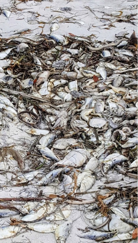
Harmful Algal Blooms (HABs) are a rapidly growing environmental concern worldwide due to their detrimental impacts on marine ecosystems, human health, and local economies. In particularly severe years, HABs can cause billions of dollars in losses. For example, in 2018 alone, damages of 2.7 billion dollars were reported in a single U.S. state—Florida¹. These blooms occur when a certain species of algae –Karenia Brevis in this case – multiply rapidly, often producing toxins that affect humans through contaminated seafood and respiratory irritation^2‘3. The frequency and severity of HABs has increased in recent decades, such as a 44% spike from the 2000s to 2010s, influenced by factors such as nutrient pollution as well as rapid increase in climate change^4‘5‘6.

In the Gulf of Mexico, particularly along the West Florida Shelf and Tampa Bay, Karenia brevis blooms (commonly known as red tides) have caused significant ecological damage and economic losses. These red tides specifically harm the tourism and fishing industries, as fish kills cause unsightly beaches and poor fishing^7‘8. Despite global trends of increasing HAB events, the frequency of regional events can differ due to local irregularities.

Machine learning (ML) has emerged as a novel approach to improve detection and prediction of HABs by utilizing large environmental datasets, including satellite remote sensing and hand sampling measurements. Studies have used ML to predict and define HABs using variables such as chlorophyll-a concentration and water temperature, including recurrent time-series models for short-term chlorophyll-a forecasting^9‘10. Comparative studies have shown that ensemble tree-based methods often outperform linear and neural-network models in short-term environmental forecasting tasks under limited data conditions, though performance varies substantially by region and feature design, particularly in operational coastal forecasting settings^11‘12‘13. Prior ML-based HAB studies have applied a range of approaches, including Random Forests, support vector machines, convolutional neural networks, and recurrent neural networks, to both bloom detection and chlorophyll-a forecasting tasks^{9‘11‘14‘15}. While these models demonstrate improved performance over traditional statistical methods, their effectiveness is often constrained by limited temporal coverage, reliance on satellite-only inputs, or lack of systematic comparison across model classes within the same study. Despite improvements, many existing ML models suffer from issues such as moderate accuracy, reliance on limited datasets, and lack of regional calibration, particularly for areas like Tampa Bay¹⁰.

Recent advances in ML-based HAB prediction have highlighted several persistent gaps. Most existing approaches depend on limited or low-frequency datasets, rely on single-source data such as satellites, and often lack regional calibration necessary for complex coastal systems. Satellite-driven ML models contribute strong spatial coverage but are frequently affected by cloud masking, optical complexity in coastal waters, and irregular sampling intervals, which reduce reliability in estuarine environments^16‘17. In contrast, in-situ and water-quality–based models offer higher temporal resolution but often suffer from sparse spatial coverage and short observational records, limiting their generalizability¹⁸. Additionally, data quality, measurement frequency, and interpretability continue to constrain operational use of ML models in management applications. Reviews emphasize the importance of developing integrated, high-quality, and explainable models tailored for specific environments to improve decision-making and predictive utility¹³.

While the use of environmental time-series data for HAB prediction is well established in the literature, key questions remain regarding optimal data integration strategies, feature engineering choices, and monitoring frequency in regionally complex systems. This study directly addresses these gaps by developing a multi-source, high-resolution HAB prediction framework tailored to Tampa Bay. It integrates in-situ, satellite, and field-sample data to overcome the limitations of single-source models and explicitly evaluates how chlorophyll-a measurement frequency affects predictive accuracy—providing quantitative guidance for monitoring design, which has been largely overlooked in prior work. Through the use of engineered temporal and threshold-based features and explainable ML (XAI) interpretation, the model enhances short-term forecasting skill and identifies interpretable environmental drivers. By focusing on local calibration, model transparency, and operational usability, this research bridges the gap between generalized ML studies and practical HAB management for regional coastal systems.

Methods

HAB Classification Framework

In this study, bloom conditions were identified using chlorophyll-a (Chl-a) concentration as a proxy for elevated phytoplankton biomass, rather than species-specific, cell-count–based bloom definitions. Chlorophyll-a was selected as the primary response variable because it is the most widely available and consistently measured indicator of phytoplankton biomass across both satellite remote sensing platforms (e.g., SeaWiFS, MODIS, VIIRS, Sentinel-3) and in-situ optical monitoring networks^2‘8. Its global coverage, multi-decadal continuity, and standardized retrieval algorithms enable scalable, automated analyses across large spatial domains and extended time periods. Consistent with this practice, a recent meta-analysis of approximately 420 peer-reviewed studies on HAB detection and monitoring identified chlorophyll-a as the most commonly used variable in remote-sensing–based HAB analyses¹⁹.

Regulatory and management agencies, including the Florida Fish and Wildlife Conservation Commission (FWC) and the Florida Department of Health (DOH), define harmful algal blooms such as Karenia brevis “red tide” using species-specific cell-count thresholds (e.g., 5 × 10³, 1 × 10⁴, and 1 × 10⁶ cells L⁻¹). However, such cell-count observations are spatially sparse, temporally irregular, and unavailable for much of the spatial and temporal extent considered in this study. As a result, the present analysis does not seek to replicate regulatory bloom classifications or to directly identify K. brevis red tide events. Instead, classification focuses on non-specific, high-biomass phytoplankton conditions that are detectable using routinely available optical data.

Chlorophyll-a–based categories were therefore employed to ensure consistent labeling across satellite-derived and in-situ optical datasets. Model training and evaluation were conducted with the explicit understanding that these categories represent phytoplankton biomass anomalies rather than taxon-specific or toxin-specific harmful algal bloom definitions.

Data

Data processing involved several steps. First, data were extracted by downloading observations from the Tampa Bay Observing Network (TBON) and NOAA remote satellite sources, then consolidated into spreadsheets.

Data Sources: TBON in-situ water quality and meteorological observations were accessed via the Tampa Bay Observing Network data portal (accessed June 2025). VIIRS chlorophyll-a products (Suomi-NPP and NOAA-20) were accessed via NOAA’s ocean color data services (accessed June 2025). A preprocessing step was subsequently applied to address data quality issues: duplicated entries were removed, and records with extended consecutive gaps were discarded, while continuous segments with valid measurements were retained. Missing values were not random but typically occurred during sensor downtime or adverse field conditions, which could introduce systematic bias if retained. For integration, the preprocessed dataset was converted from spreadsheets to CSV files and organized into folders by station identifier. The files were then categorized by measurement type as either water quality or meteorological data. Finally, a nearest neighbor interpolation technique was applied to generate a continuous dataset across sampling locations and times. This technique assigns each unsampled point the value of the nearest valid observation in multi-dimensional space, based on geographic coordinates and time, thereby producing a uniform and spatially coherent dataset suitable for model development.

Satellite Data Processing and Quality Control

We used satellite chlorophyll-a data from the VIIRS sensor on the Suomi NPP and NOAA-20 satellites. This data went through the standard process of the OCx blue–green band-ratio algorithm along with NOAA’s operational atmospheric correction.

The process masks pixels that fail basic quality checks, including those affected by clouds, high glint, invalid atmospheric correction, or low radiance. In this study, we relied on these default NOAA filters and thus used their filtered measurements. No other manual filters were applied.

Because Tampa Bay contains shallow, optically complex waters, some pixels were still unavailable after NOAA’s automated masking. These masked regions naturally remained excluded from analysis, and only the remaining valid pixels were used. This step reduced data quantity drastically, but was essential for obtaining only clean data.

After quality filtering via the NOAA Level-2 product, each satellite pixel was matched to TBON in-situ samples using nearest-neighbor interpolation. The closest valid pixel based on location and time was paired with hand-sampled data to create a table that combined engineered features, in-situ data, and satellite measured data.

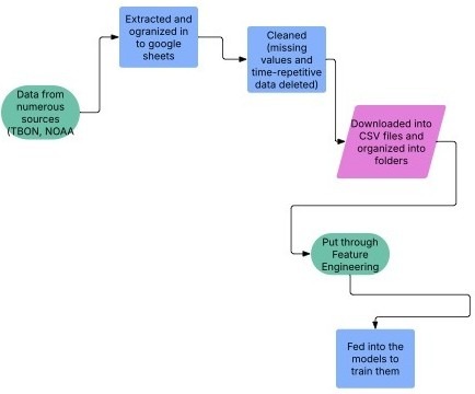
Figure 2 illustrates the end-to-end data pipeline used in this study. Raw in-situ water quality, meteorological, and satellite observations were first quality-controlled and temporally aligned, followed by feature engineering to generate lagged, rolling, and threshold-based predictors. The processed dataset was then used to train and evaluate regression and classification models for chlorophyll-a prediction and HAB detection.

As shown in the top of Figure 3, the temporal variability of chlorophyll-a was examined for one of the five monitored sites in the Tampa Bay Area, covering the period from April 2023 through July 2025. The time series reveals pronounced peaks and troughs in algal biomass, reflecting episodic growth events likely influenced by hydrological, meteorological, and nutrient-loading conditions. Similar trends were observed across the other four sites.

Complementing the temporal analysis, the two comparative plots in the lower panels of the same figure present the relationships between chlorophyll-a and key environmental parameters: water temperature and dissolved oxygen saturation. The scatterplots indicate that chlorophyll-a dynamics exhibit a nonlinear association with either variable. These patterns highlight the complexity of algal dynamics in estuarine systems and suggest the necessity of employing more advanced mathematical models to unravel the multivariate interactions and improve predictive performance of chlorophyll-a concentration.

Feature Engineering:

As part of the data preparation process aimed at identifying the most influential factors in predicting chlorophyll-a concentrations, extensive feature engineering procedures were implemented to enhance the explanatory power of the dataset. This process substantially expanded the set of predictor variables available to the machine learning (ML) algorithm. Specifically, the initial nine variables were systematically transformed into a feature space exceeding one hundred variables through the application of temporal lags, as well as the computation of rolling statistics such as moving averages, minima, and maxima. These transformations allowed the model to capture both short- and long-term dependencies in the data, thereby improving its capacity to represent underlying dynamics.

The use of lag-based variables was also motivated by similarities to other fields where past system states are strong predictors of future outcomes. In weather forecasting, for example, current atmospheric conditions often inform short-term predictions, with rainfall today increasing the likelihood of rainfall tomorrow²⁰. In medical diagnosis, previous cardiac events are frequently used to estimate the risk of future incident²¹. By drawing on these established principles, temporal lag features were incorporated to capture comparable autoregressive patterns in chlorophyll-a dynamics.

Additionally, threshold variables were introduced to identify instances where water temperatures exceeded 60 degrees F and chlorophyll-a values exceeded 40 mg/m³, indicative of bloom conditions. A detailed inventory and description of the resulting feature set, including original variables, derived lagged metrics, and threshold indicators, is provided in Table 1

Models were trained on varying degrees of the feature engineering, including without threshold variables, with all threshold variables, and with threshold variables measured every 24 hours.

The time series data was split to ensure accurate training and testing. The training spanned from 2023 to February of 2025, and the testing data spanned from February 2025 to August 2025. Additionally, the testing set was partially composed of a brand-new site: Tampa Bay Observing Network Site 08. This site was not part of the training set and entirely used for testing, showcasing how the model can be generalized on new sites in the Tampa Bay area.

Feature Name	Description	Units	Type	Raw / Feature Engineering	Source
water_temperature*	Temperature of the water at the bottom	°F	float	raw data	Tampa Bay observing network
air_temperature	Measured air temperature	°F	float	raw data	Tampa Bay observing network
dissolved_oxygen *	Amount of oxygen in the water	ppm	float	raw data	Tampa Bay observing network
oxygen_saturation *	Ratio of dissolved oxygen to the max oxygen the water can hold	%	float	raw data	Tampa Bay observing network
chlor_f *	Measured red light emitted by chlorophyll molecules	ppb	float	raw data	Tampa Bay observing network
wind_direction*	Degrees north that wind is blowing	degrees	float	raw data	Tampa Bay observing network
wind_speed*	Measured wind speed	mph	float	raw data	Tampa Bay observing network
salinity*	Measured dissolved salt in the water	PSU	float	raw data	Tampa Bay observing network
humidity*	Measured water vapor in the air	%	float	raw data	Tampa Bay observing network
Phycoerythrin*	Measure of the emitted light from Phycoerythrin molecules	ppb	float	raw data	Tampa Bay observing network
Above_threshold_chlor_a_avg_12h **	A 0 or 1 value depending on if a chlorophyll-a value in the past 12 hours was above 40 mg/m3	N/A	float	feature-engineered
Above_threshold_water_temp_12h **	A 0 or 1 value depending on if the water temp in the past 12 hours was above 60 degrees F	N/A	float	feature-engineered
water_temperature_avg12h	Average temperature of the water in the last 12 hours	°F	float	feature-engineered
water_temperature_avg24h	Average temperature of the water in the last 24 hours	°F	float	feature-engineered
water_temperature_avg48h	Average temperature of the water in the last 48 hours	°F	float	feature-engineered
water_temperature_min12h	Minimum temperature of the water in the last 12 hours	°F	float	feature-engineered
Water_temperature_max12h	Maximum temperature of the water in the last 12 hours	°F	float	feature-engineered

* Average values, minimum, and maximum were also estimated for the rest of the parameters. Values were spaced at 12, 24, and 48 hr intervals.
** This variable was also calculated for 24, 48, and 72hr

AI Models Implementation

The artificial intelligence (AI) approach was designed to address two related predictive tasks: (i) forecasting continuous chlorophyll-a concentrations and (ii) detecting the occurrence of harmful algal blooms (HABs). To evaluate model performance across both regression and classification contexts, a series of machine learning (ML) algorithms were implemented.

For the regression task, chlorophyll-a concentrations were treated as a continuous response variable. The modeling process began with a baseline linear regression model, followed by a regularized regression approach (Lasso), a feed-forward artificial neural network (ANN), and a gradient-boosting model (XGBoost). This sequence allowed for systematic comparison across models of varying complexity and capacity for capturing nonlinear interactions.

Then, hyperparameter optimization was conducted for the XGBoost using grid search and randomized search procedures were applied to tune key parameters, such as the maximum depth, learning rate, and number of estimators. Model selection was based on minimizing error metrics for regression.

Additionally, an alternative implementation of the XGBoost model was tested using a reduced predictor set. This subset removed features engineered to capture recent HAB conditions, of. The goal of this experiment was to assess whether emphasizing predictors directly linked to lagged indicators of elevated chlorophyll-a improved the prediction performance relative to models trained on a more limited feature set.

For the classification task, chlorophyll-a concentrations were evaluated using a threshold of 40 mg/m³, a value commonly associated with bloom conditions. A Random Forest classifier was trained to predict bloom versus non-bloom states, enabling assessment of model robustness in distinguishing ecologically critical events.

A brief description of the models used is below:

Regression Models:

Initial regression models were applied to predict continuous chlorophyll-a concentrations:

1. Linear Regression: Multivariate ordinary least squares (OLS) regression was used as a baseline model to estimate linear relationships between chlorophyll-a concentration and environmental predictors by minimizing the residual sum of squares. This model assumes additive effects and serves as a benchmark for evaluating the benefits of nonlinear approaches.`
2. XGboost: Extreme Gradient Boosting (XGBoost) was applied as an ensemble of decision trees optimized via gradient descent on a regularized objective function. This approach efficiently captures nonlinear interactions and temporal dependencies among environmental variables while controlling model complexity through built-in regularization.
   
   
3. Lasso Regression (regularization): Lasso regression extends linear regression by incorporating an L1 regularization penalty, which shrinks less informative coefficients toward zero and performs implicit feature selection. This approach reduces overfitting in high-dimensional feature spaces generated through extensive temporal feature engineering.

A feed-forward artificial neural network (ANN) was implemented to capture nonlinear relationships between predictors and chlorophyll-a concentration through multiple hidden layers and nonlinear activation functions. Model complexity was constrained to mitigate overfitting given the limited temporal extent of the dataset.

Classification Models

A Random Forest classifier was used to predict bloom versus non-bloom conditions by aggregating predictions from an ensemble of decorrelated decision trees trained on bootstrap samples. This ensemble approach reduces variance and improves robustness in binary classification of harmful algal bloom events.

Model performance was evaluated using chronological train–test splitting to preserve temporal dependence, with stratified sampling applied only within bootstrap resampling for classification performance analysis.

Model Evaluation

The performance of regression models was evaluated using the following error metrics:

Mean Absolute Error (MAE):

(1)  

Root Mean Squared Error (RMSE):

(2)  

Mean Absolute Percentage Error (MAPE):

(3)  

Symmetric Mean Absolute Percentage Error (SMAPE):

(4)  

The classification models were evaluated using accuracy, F1-score, and confusion matrices to assess the model’s ability to correctly categorize HAB severity. This structured methodology ensures that both continuous and categorical predictions of HABs are rigorously evaluated, while leveraging multiple data sources and advanced AI techniques to maximize predictive accuracy.

Model Selection Rationale

The models chosen for this study—linear regression, Lasso, ANN, XGBoost, and Random Forest—were selected to have a broad spectrum from simple, linear models to more advanced models commonly used in environmental settings. These models were prioritized because they balance performance, interpretability, and mesh well with the data we were working with.

More advanced deep learning approaches such as LSTM networks or spatial graph neural networks were not employed for two reasons. First, the data was restricted by its short timeframe as the TBON hand-sampling stations only overlapped with the NOAA chlorophyll-a data (2023-2025) which would hinder the effectiveness of these models. Secondly, the study sought to provide readable data for scientists and environmentalists rather than complex, uninterpretable data. This rationale led us to choose our models (XGBoost, Random Forest), rather than more advanced deep learning approaches.

The extensive use of lagged and rolling features introduces potential multicollinearity and increases the risk of overfitting. However, this risk was mitigated through the use of regularized models (Lasso), tree-based ensemble methods (XGBoost and Random Forest), and strict temporal train–test separation, all of which are known to be robust to correlated predictors.

Lasso and XGBoost Hyperparameter Tuning

LASSO hyperparameters were optimized using Bayesian optimization with the Optuna Python library, where the regularization parameter α was sampled from a log-uniform distribution. The optimal value of α was determined using 5-fold cross-validation, selecting the parameter that minimized the mean squared error on the validation set. Table 1 presents the hyperparameter search space and the final value selected.

Hyperparameter	Search distribution	Max Iterations	Trials / Evaluations	Selected value
α (LASSO)	log [1e-6, 1e1]	5,000	50	0.74

To identify the optimal configuration of the XGBoost model, we performed hyperparameter tuning using the Hyperopt Python library. The Tree-Structured Parzen Estimator (TPE) algorithm was employed due to its efficiency compared to grid or random search. The objective of the optimization was to minimize the Root Mean Squared Error (RMSE) on the validation set, using uniform probability distributions to sample each hyperparameter. The search space covered key XGBoost hyperparameters, including the learning rate, tree depth, and regularization coefficients. Table 1 shows the full search ranges and the final values selected by this process.

Hyperparameter	Search Range / Candidate Values	Selected Value
n_estimators	50–500	300
learning_rate	0.01 – 0.3	0.01
max_depth	3–10	5
min_child_weight	1-10	9
subsample	0.5–1.0	0.79
colsample_bytree	0.6–1.0	0.75
gamma	0–0.5	0.29
reg_alpha	{0.0, 0.01, 0.1-1}	0.60
reg_lambda	0.1-2.0	0.48
eval_metric	–	RMSE

Artificial Neural Network Architecture

The ANN architecture consisted of an input layer with 147 features, followed by two hidden layers. The hidden layers used ReLU activation function and contained 32 and 16 neurons, respectively. A dropout rate of 0.3 was applied after each hidden layer to reduce overfitting. The output layer consisted of a single neuron with a linear activation function. Training was conducted using the Adam optimizer with a learning rate of 0.001, a batch size of 32, and a maximum of 100 epochs. The mean squared error (MSE) was used as the loss function.

Results

Model Performance

All of the models performed poorly with no chlorophyll threshold variables. The majority produced a root mean squared error (RMSE) of around 27. However, the linear regression model produced a RMSE of 35.2, making it the worst performing model with no chlor-threshold variables. When all threshold variables were introduced with no tuning, the XGboost model performed the best (RMSE = 14.557), and the ANN performed the worst (RMSE = 22.2). Then, hyperparameters were introduced for model tuning on the XGboost model, which produced the lowest RMSE of all the models (13.67).

ML Model	Model Version	Tuned/ No tuned	MSE	RMSE	MAE	MAPE	SMAPE	R2
Lasso	All Variables	no tuned	214.482	14.645	12.119	0.771	44.689	0.674
	No Chlorophyll threshold variables	No tuned	734.027	27.093	21.941	1.571	66.469	-0.115
ANN	All Variables	No tuned	494.718	22.242	17.919	1.435	57.072	0.249
	No Chlorophyll threshold variables	No tuned	746.498	27.322	22.185	1.618	70.215	-0.133
Linear Regression	All Variables	No tuned	285.603	16.900	13.361	0.806	52.663	0.566
	No Chlorophyll threshold variables	No tuned	1238.574	35.193	23.981	1.387	74.225	-0.881
XGBoost	All Variables Included	no tuned	211.896	14.557	12.160	0.731	47.437	0.678
		tuned	186.882	13.670	11.263	0.670	44.423	0.716
	Only with 48h and 72h Clor-a threshold*	no tuned	318.595	17.849	14.020	0.893	50.258	0.516
		tuned	266.255	16.317	12.492	0.813	45.720	0.596
	No Chlorophyll threshold variables	no tuned	751.839	27.420	22.154	1.466	68.568	-0.142
		tuned	659.681	25.684	20.658	1.506	64.139	-0.002

* This degree of feature engineering can be applied to all models, but all models follow the same pattern, as more and more frequent chlor-a measurements are made, less error is produced.
**MAPE values may be higher than expected due to the majority of chlorophyll-a data being close to 0, thus creating disproportionally high MAPE values. Chlorophyll-a tends to range from 0-100 mg/m³. SMAPE is a better gauge.

Several baseline models produced negative R² values when chlorophyll-a threshold variables were excluded, indicating performance worse than a naïve mean predictor and highlighting the limited explanatory power of physical and meteorological variables alone.

Table 6 shows the top 10 most important variables in the initial feature engineering stage versus the final stage alongside their respective importance.

Statistical Comparison of Machine Learning Models Using Bootstrap Resampling

Bootstrap resampling was applied to the test data subset to evaluate and compare the predictive performance of the ANN, XGBoost, and Lasso models using all available predictor variables, and a reduced predictor set excluding chlorophyll threshold variables. For each bootstrap iteration, RMSE values were computed, generating empirical performance distributions for each model (Figure 1). The analysis reports comprehensive descriptive statistics to summarize the central tendency and variability of model performance. Table 5 presents the descriptive statistics of the bootstrap RMSE distributions for all models and predictor configurations.

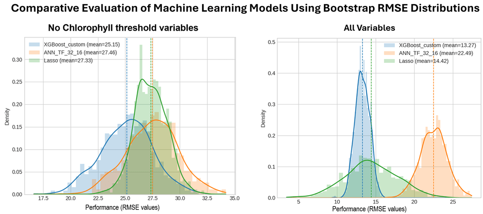
Then, pairwise comparisons between models were conducted using Wilcoxon signed-rank tests applied to the bootstrap RMSE distributions. Conventional cross-validation approaches were not employed because the data are structured as a time series, and random or k-fold splitting would violate the temporal dependence among observations.

Model Version	No Chlorophyll Threshold Variables			All Variables
Variable/Model	XGB	Lasso	ANN	XGB	Lasso	ANN
N	1000	1000	1000	1000	1000	1000
Minimum	16.64	22.36	18.89	11.06	2.92	17.08
Maximum	31.98	32.23	34.21	15.70	24.63	28.05
Mean	25.15	27.33	27.46	13.62	14.60	22.61
Median	25.26	27.29	27.53	13.59	14.59	22.60
Std. Dev.	2.38	1.49	2.38	0.69	3.44	1.89

For the models excluding chlorophyll threshold variables, the Wilcoxon signed-rank tests reveal clear but differentiated performance differences among the three machine learning models. The comparison between XGBoost and ANN yields an extremely small p-value (3.33 x 10^-165) with a test statistic of 0.0, indicating a perfectly consistent difference across all paired samples and providing overwhelming evidence that XGBoost outperforms ANN. The XGBoost–Lasso comparison is also highly significant (p=5.24 x 10^-95), demonstrating a robust performance advantage for XGBoost, although with greater variability in the paired differences. In contrast, the ANN–Lasso comparison does not reach statistical significance at the 5% level (p=0.0555), suggesting comparable predictive performance between these two models under this predictor configuration. Overall, these results identify XGBoost as clearly superior, while ANN and Lasso exhibit similar performance when chlorophyll threshold variables are excluded.

When all chlorophyll variables are included, the Wilcoxon test results provide very strong evidence of performance differences among all three models. As before, XGBoost significantly outperforms ANN (p=3.33 x 10^-165, statistic = 0.0), indicating complete consistency across resamples. Significant differences are also observed between XGBoost and Lasso (p=8.82 x 10^-16) and between ANN and Lasso (p=6.27 x 10^-164), demonstrating clear separation in predictive performance across all model pairs. In general, these findings indicate a well-defined performance ranking when chlorophyll variables are included, with XGBoost, ANN, and Lasso each exhibiting statistically distinct predictive behavior.

Variable (initial feature engineering stage )	Importance	Variable (final feature engineering stage)	Importance
avg_water_temp_12h	0.023419	above_threshold_chlor_a_avg_12h	0.314171
max_phycoerythrin_f_12h	0.019442	above_threshold_chlor_a_avg_24h	0.265406
site_name_TB04	0.018413	above_threshold_chlor_a_avg_48h	0.074527
avg_water_temp_48h	0.01671	above_threshold_chlor_a_avg_72h	0.009485
min_oxygen_saturation_72h	0.016203	max_salinity_24h	0.007957
max_oxygen_saturation_72h	0.015163	max_salinity_72h	0.007422
avg_water_temp_72h	0.014273	avg_salinity_72h	0.006438
wind_direction	0.013902	max_salinity_48h	0.006384
avg_air_temp_48h	0.01377	min_water_temp_24h	0.005874
avg_phycoerythrin_f_72h	0.013262	salinity	0.005522

Figure 5 depicts varying levels of threshold data in the XGboost models and the subsequent variable importance through SHAP plots. On the far left, a SHAP plot is made assuming no past chlorophyll-a data is measured and thus is purely predictive. The middle plot assumes a measurement of chlor-a every 48 hours. The far-right plot is the SHAP figure for the most informed model with chlor-a measurements coming in every 12 hours. With no chlor threshold variables, the most important predictors are the phycoerythrin levels, wind speed, and air temp. When chlor variables are measured every 48 hours, the most important variables change to the 48 hour chlor threshold, the 72 hour chlor threshold, and the phycoerythrin levels. Lastly, taking chlor measurements every 12 hours, the most predictive variables changed to the 12 hour chlorophyll threshold, the 48 hour chlor threshold, and the 72 hour chlor threshold.

These persistence features are included intentionally to quantify how monitoring frequency improves short-term forecast skill; models excluding chlorophyll history represent ‘driver-only’ prediction and perform substantially worse.

Classification Results

Data from beforehand coupled with feature engineering improved accuracy significantly.

A random forest classifier was implemented to evaluate the contribution of chlorophyll-a threshold variables to model performance, with a random classifier baseline using a chlorophyll-a threshold of 40 mg/m³. By incorporating chlorophyll-a thresholds at different temporal lags (72 h, 48 h, and 24 h), the random forest framework allows a systematic assessment of how additional chlorophyll information improves event detection and overall classification quality.

Figure 6 summarizes the performance of the different model configurations and includes both the evaluation metrics and the corresponding confusion matrices. As shown in the figure, the model without any chlorophyll thresholds performs poorly, particularly in recall (0.0196) and F1-score (0.037), indicating that it almost completely fails to detect positive cases. Adding the 72-hour chlorophyll-a threshold substantially improves all metrics, with accuracy rising to 0.7483 and a large gain in precision (0.7826), although recall remains relatively limited (0.3529), suggesting many missed events. The performance improves dramatically when both 48-hour and 72-hour thresholds are included: accuracy exceeds 0.92, recall increases to 0.9804, and the F1-score reaches 0.9009, indicating a strong balance between precision and recall. The best overall performance is achieved when 24-hour, 48-hour, and 72-hour chlorophyll-a thresholds are all included, yielding the highest accuracy (0.947), perfect recall (1), and the highest F1-score (0.9273).

Finally, to verify that the classification model performance was not driven by data leakage, a comprehensive data leakage analysis was conducted to ensure that target-related or future information was not incorporated during model training, which could lead to artificially inflated accuracy and poor generalization. This assessment evaluated the same configurations presented in Figure 5. The model without Chl-a threshold variables exhibited lower predictive performance and no indicators of leakage, suggesting that its predictions were derived solely from the explanatory variables used in training. In contrast, the inclusion of the 48-hour lagged chlorophyll-a threshold resulted in a marked increase in predictive performance but was accompanied by pronounced feature dominance by this variable and high single-feature predictive power, indicating that this variable may capture information temporally proximal to the target outcome. The model incorporating a 72-hour lagged threshold achieved improved performance relative to the baseline while avoiding the extreme feature dominance observed at shorter lags.

The leakage analysis was implemented using a time-series-aware validation framework that enforced strict temporal separation between training and testing datasets and was complemented by label-shuffling tests, duplicate-sample detection across splits, single-feature predictive assessments, and permutation-based importance evaluation on held-out data. Collectively, these results indicate that shorter lagged threshold variables are more susceptible to implicit temporal leakage, whereas longer lag definitions provide a more methodologically robust balance between predictive performance and generalizability, thereby enhancing confidence in the model’s applicability to real-world prediction tasks.

Discussion

Our models demonstrated that combining multiple environmental datasets—Tampa Bay Observing Network (TBON) water quality, NOAA satellite observations, and Florida Fish and Wildlife Conservation hand-collected samples—improves short-term prediction of high-biomass phytoplankton events in Tampa Bay. Among all algorithms evaluated, XGBoost consistently outperformed Linear Regression, Lasso, and ANN. This was expected as we knew that the prediction would likely not be a linear problem and that the relatively short dataset limits neural-network performance. Since gradient-boosted trees can capture data interactions and shifts that linear models cannot as well as being able to work in the relatively short timeframe, it was expected that this approach would provide better results. The Random Forest classifier also achieved strong accuracy in distinguishing bloom vs. non-bloom states. This led us to believe that a categorical based approach aligns well with decision tree results. Model performance increased with the introduction of threshold values. Thresholds included water temperature (if temperatures exceeded 60 degrees fahrenheit in a given time period) as well as chlorophyll-a thresholds (when it exceeded 40 mg/m³). The models performed better with more frequent measurements of chlorophyll-a.  The strong dependence on 12–48-hour chlorophyll thresholds indicates that bloom behavior in Tampa Bay is highly path-dependent, where recent biomass levels carry more predictive information than physical drivers alone. This explains why models relying only on water-quality and meteorological variables produced higher errors (RMSE ≈ 25), while models with frequent chlorophyll-a measurements performed substantially better. The occurrence of negative R² values in baseline regression models further underscores that short-term chlorophyll-a dynamics in Tampa Bay cannot be adequately captured without recent biological context, reinforcing the necessity of threshold-based and lagged chlorophyll predictors. These results highlight the utility of integrating diverse datasets with advanced machine learning approaches for HAB prediction. Accurate forecasting can support environmental management decisions, such as issuing public health warnings and guiding resource allocation for fisheries and tourism. The framework developed here can serve as a region-specific tool for Tampa Bay, addressing limitations in prior models that lacked local calibration and sufficient temporal coverage.

The continuous and categorical predictions generated by this framework provide interpretable information about the occurrence as well as the severity of blooms for interested environmental parties.  Rather than generalizing beyond Tampa Bay, these results show the importance of region-specific calibration and demonstrate which variables are most influential for short-term HAB forecasting. These are recent biological conditions, followed by optical and water-quality indicators.

Future research should explore longer-term datasets and additional environmental factors, including nutrient runoff and hydrodynamic variables, to further enhance predictive performance. Deploying real-time data feeds could enable dynamic forecasting, benefiting both local authorities and the public.

This study has several limitations that should be acknowledged. The relatively short temporal coverage (2023–2025) increases the potential for model overfitting, particularly for high-capacity models such as XGBoost, despite the use of regularization, chronological train–test splitting, and evaluation on an unseen monitoring site. Additionally, while temporal ordering was preserved, the analysis lacks multi-year temporal validation, limiting confidence in model performance under interannual climate variability or extreme bloom conditions not represented in the dataset. Finally, the models provide point predictions and binary classifications but do not include formal uncertainty quantification(e.g., prediction intervals or probabilistic forecasts), which would be valuable for operational decision-making. Satellite data limitations related to cloud cover and optical complexity in shallow estuarine waters may further contribute to uncertainty.

Additionally, a limitation of this study is the use of chlorophyll-a as a proxy for HAB detection and classification. Chlorophyll-a represents total phytoplankton biomass and does not distinguish taxa or toxicity, such that high concentrations may reflect non-harmful blooms, while some HAB events can occur at high cell densities but low chlorophyll-a levels. Consequently, regulatory agencies define HAB severity using species-specific cell-count thresholds rather than chlorophyll-based metrics. The classifications presented here should therefore be interpreted as indicators of elevated phytoplankton biomass rather than definitive HAB occurrence. This reflects a deliberate trade-off to enable scalable, automated analysis, as cell-count observations are spatially sparse and temporally irregular compared to routinely available chlorophyll-a products. Future work should integrate cell counts and complementary optical proxies where available to strengthen species-specific attribution.

By combining AI methods with multi-source environmental datasets, this study clarifies the mechanisms most essential to near-term HAB prediction in Tampa Bay and provides a foundation for improving monitoring strategies. While additional variables are needed for broader generalization, the insights presented here contribute to a more evidence-based approach to managing harmful algal blooms in this region.

References

1. Hernández‐Brito, J.J., Louzao, M., Fernández, R., & Arístegui, J. (2024). Socioeconomic impacts of harmful algal blooms: A global perspective. Journal of Environmental Management, 352, 119989 [↩]
2. D. M. Anderson, P. M. Glibert, J. M. Burkholder. Harmful algal blooms and eutrophication: examining linkages. Harmful Algae. Vol. 8(1), 39–53, 2012 [↩] [↩]
3. P. Hoagland, D. M. Anderson, Y. Kaoru, A. W. White. The economic effects of harmful algal blooms in the United States: estimates, assessment issues, and information needs. Estuaries. Vol. 25(4), 819–837, 2002 [↩]
4. L. Feng, Y. Wang, X. Hou, B. Qin, T. Kuster, F. Qu, N. Chen, H. W. Paerl, C. Zheng. Harmful algal blooms in inland waters. Nature Reviews Earth & Environment. Vol. 5(9), 631–644, 2024. doi:10.1038/s43017-024-00578-2 [↩]
5. G. M. Hallegraeff. A review of harmful algal blooms and their apparent global increase. Phycologia. Vol. 32(2), 79–99, 1993 [↩]
6. C. J. Gobler, O. M. Doherty, T. K. Hattenrath-Lehmann, A. W. Griffith, Y. Kang, R. W. Litaker. Ocean warming since 1982 has expanded the niche of toxic algal blooms in the North Atlantic and North Pacific oceans. Proceedings of the National Academy of Sciences. Vol. 114(19), 4975–4980, 2017 [↩]
7. P. A. Tester, K. A. Steidinger. Gymnodinium breve red tide blooms: initiation, transport, and consequences of surface circulation. Limnology and Oceanography. Vol. 42(5), 1039–1051, 1997 [↩]
8. R. M. Kudela, S. Seeyave, W. P. Cochlan. The role of nutrients in regulation and promotion of harmful algal blooms in upwelling systems. Oceanography. Vol. 28(2), 58–69, 2015 [↩] [↩]
9. F. N. Yussof, N. Maan, M. N. Md Reba. LSTM networks to improve the prediction of harmful algal blooms in the west coast of Sabah. International Journal of Environmental Research and Public Health. Vol. 18(14), 7650, 2021 [↩] [↩]
10. J. P. Cannizzaro, K. L. Carder, F. E. Muller-Karger, C. A. Heil. Detection of Karenia brevis blooms on the west Florida shelf using in situ backscattering and fluorescence data. Harmful Algae. Vol. 8(1), 90–105, 2009 [↩] [↩]
11. Y. Zhang, X. Liu, Y. Wang, Y. Chen. Prediction of harmful algal blooms using random forest and support vector machine models. Ecological Indicators. Vol. 125, 107489, 2021 [↩] [↩]
12. R. P. Stumpf, M. C. Tomlinson, J. A. Calkins, B. Kirkpatrick, K. Fisher, K. Nierenberg, R. Currier, T. T. Wynne. Skill assessment for an operational algal bloom forecast system. Journal of Marine Systems. Vol. 76(1–2), 151–161, 2009 [↩]
13. B. Z. Demiray, O. Mermer, Ö. Baydaroğlu, I. Demir. Predicting harmful algal blooms using explainable deep learning models: a comparative study. Water. Vol. 17(5), 676, 2025 [↩] [↩]
14. C. Hu, J. Cannizzaro, K. L. Carder, F. E. Muller-Karger, R. Hardy. Remote detection of Trichodesmium blooms in optically complex coastal waters: examples with MODIS full-spectral data. Remote Sensing of Environment. Vol. 114, 2048–2058, 2010 [↩]
15. F. Recknagel. Applications of artificial neural networks in limnology. Ecological Modelling. Vol. 146(1–3), 111–124, 2001 [↩]
16. M. Izadi, M. Sultan, R. E. Kadiri, A. Ghannadi, K. Abdelmohsen. A remote sensing and machine learning-based approach to forecast the onset of harmful algal bloom. Remote Sensing. Vol. 13(19), 3863, 2021 [↩]
17. P. J. Werdell, L. I. W. McKinna, E. Boss, S. G. Ackleson, S. E. Craig, W. W. Gregg, Z. Lee, S. Maritorena, C. S. Roesler, C. S. Rousseaux, D. Stramski, J. M. Sullivan, M. S. Twardowski, M. Tzortziou, X. Zhang. An overview of approaches and challenges for retrieving marine inherent optical properties from ocean color remote sensing. Progress in Oceanography. Vol. 160, 186–212, 2018 [↩]
18. J. Park, K. Patel, W. H. Lee. Recent advances in algal bloom detection and prediction technology using machine learning. Science of the Total Environment. Vol. 938, 173546, 2024 [↩]
19. M. Salehi, G. Mountrakis. A meta-analysis of remote sensing of harmful algal blooms. Remote Sensing. Vol. 13(8), 1404, 2021 [↩]
20. G. E. Box, G. M. Jenkins, G. C. Reinsel, G. M. Ljung. Time series analysis: forecasting and control. Wiley, 2015 [↩]
21. E. J. Benjamin, P. Muntner, A. Alonso. Heart disease and stroke statistics—2019 update. Circulation. Vol. 139(10), e56–e528, 2019 [↩]