
Abstract
This research investigated how timing variability changed within and across trials as a function of practice. The exploratory single-participant case study was conducted, and an 11-note guitar melody was chosen and played by a single participant fifty-five times. All the performance trials were recorded and analyzed for the timing consistency of each note played. Using audio-based analysis, the timing intervals between consecutive notes were quantified. The analyses were done by implementing the obtained data into different comparisons (the differences in melody duration) and statistical measurements (standard deviation (S.D.), coefficient of variation (C.V.)). These findings described timing stabilization in a musical motor task related to the practice. Based on the idea that the skill should improve over time, several hypotheses were proposed. Specifically, with practice, timing consistency became more stable, as the duration of the whole melody decreased over practice (average duration dropped from 8 to 6 seconds). Moreover, the drop in C.V. and S.D. values from 0.34 to 0.13, and from 0.26 to 0.08, respectively, may have reflected increased consistency of performance. While some results showed clear trends, others did not demonstrate a consistent pattern (for example, variability of note timing within trials fluctuated as the song progressed). This experiment contributed to the understanding of motor skill learning in humans by providing a multi-metric analysis from a repeated-measures single-subject dataset. Although no neural data were included, the observed behavioral patterns were discussed in relation to existing theoretical frameworks of variability reduction with practice. Due to the single-participant design, this project was aimed towards the acquisition of data and data analysis for the purpose of hypothesis generation for future studies.
Keywords: motor learning, timing variability/consistency, guitar practice, case study, skill improvement, trial and error.
Introduction
How living beings learn.
From the earliest times, living beings have been prone to learn new skills. Some behaviors, however, are innate and do not require learning. For example, reflexes — such as sucking or blinking, which are present at birth, are thought to result from evolutionary processes, becoming encoded in the nervous system over generations1. They are examples of innate skills that do not require practice or learning, serving as essential responses to the environment.
Motor learning, trial-and-error variability
In contrast, skills that require thinking and learning, such as speaking or playing a musical instrument, are acquired through motor learning processes, a process through which practice leads to improvements in skill learning2,3. The first important part of motor learning is variability, which enables exploration of motor solutions 4. For example, refinements in timing consistency and the reduction of temporal variability across repeated actions5, are all connected to motor learning.
One natural example of motor learning is learning to speak. Although speech differentiates us from other living beings, the learning process itself is surprisingly similar to that of other species, because all brains share common organizational mechanisms. First, infants listen to adult speech, storing it in memory as a “target model.” Then they engage in a trial-and-error process. Through babbling, they gradually experiment with opening their mouths and moving their tongues to approximate the sounds they have heard. These actions are spontaneous variations (trials), as the variability is the key part of the motor learning process. Since it is impossible to imitate the target model from the first time, the brain tries to explore all possible movements and vocal patterns without knowing in advance which will give the best outcome6. This active exploration is the first ingredient of trial-and-error learning: the brain generates many variable attempts, which then become subject to improvement7. Considering our following experiment, musical practice also could be a part of motor learning, as an activity that requires practice over time8.
Dopamine and reinforcement learning
Dopamine is commonly known as the “pleasure neurotransmitter,” released when we drink coffee or watch a good movie. But in fact, its function is much broader. Dopamine can act as a biological marker of success and error, guiding the brain in deciding which actions to repeat and which to avoid9. Its signals can strengthen neural connections for successful actions and weaken those for unsuccessful ones, a process known as synaptic plasticity10.
Returning to the speech example: when an infant’s sound, produced in a trial, resembles the adult’s model, dopamine release strengthens the neural connections that produced that attempt, “highlighting” it for future repetition. Conversely, when a sound fails to match the model, becoming an error, dopamine release decreases, and the associated connections are weakened. In this way, dopamine functions as an internal evaluation system, reinforcing correct actions and discouraging ineffective ones9,11.
As was mentioned above, the process of learning a language in humans is not very different from that of animals; a similar mechanism can be observed in how songbirds learn to sing. Juvenile birds listen to adult songs, memorize them as a template, and then repeatedly attempt to reproduce them. Each attempt is evaluated, distinguishing good trials and errors, and dopamine release determines which vocal patterns are reinforced11. Over time, the bird’s song converges on the adult model. Additionally, this process illustrates that reinforcement learning is not only related to humans but could be common across other species.
Timing and cerebellum
In musical performance, precise timing and synchronization with an external rhythm are essential for skilled execution12,13. Therefore, in the following experiment, timing might play one of the crucial roles in skill acquisition.
Timing — is the ability of the brain to correctly code the sequence of events and understand movements in time14. Rather than relying on a single internal clock, timing emerges from distributed neural network activity across multiple brain systems. In the upcoming experiment, timing ability might determine how quickly finger movements are executed and how consistent the intervals between notes remain across trials.
Different forms of timing contribute to skilled performance. Sensory timing supports perception of durations and intervals, allowing individuals to estimate how long a sound lasts or how much time has passed between events15. Motor timing controls the skill execution, determining when an action should begin and how long it should be maintained16. However, while playing a melody the predictive timing plays a crucial role, helping foretell when the anticipated event will happen which is not a full reaction. Importantly, predictive timing, which enables anticipation of upcoming events14, is critical in tasks such as musical performance where actions must be synchronized with expected temporal structures.
Timing is also highly dependent on cerebellum, which is associated with temporal precision, error correction, and movement smoothness17. The cerebellum processes a specific type of error signal that specifies how the error should be corrected. This process is called supervised learning. For example, if a person throws a dart and misses right, he will know that the next throw needs to be more left. This is the key to a supervised error signal – it instructs what needs to be done to fix the error.
Together, these processes form an integrated system that underlies skill acquisition. Their coordinated interaction enables the gradual development and refinement of complex behaviors.
Methods
Experiment
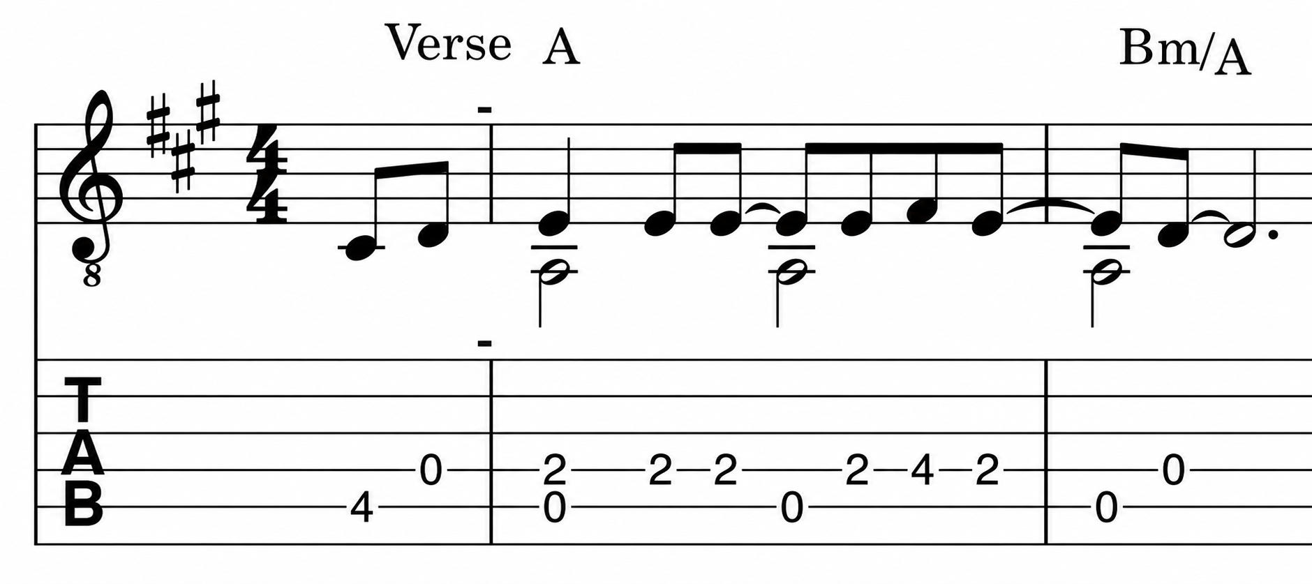
An experiment was created by learning an appropriate melody on the guitar and recording the performances along the way to analyze them after. The goal of this experiment was to precisely quantify motor performance and identify hallmarks of behavioral improvement with practice. So, the performer was a single participant (a 15-year-old girl with 2 years of nonconstant practice of playing on the guitar as a hobby), without any musical education.The chosen piece of song was “Circle of Life” by Elton John, from “The Lion King” soundtrack. The opening part, consisting of 11 notes, was recorded during the process of learning this melody.
Critically, no neuronal or dopaminergic mechanisms data were collected, so the results were acquired to test behavioral predictions of motor learning theory and to provide hands-on experience in original data acquisition and analysis.
Fifty-five trials were selected as the total number of performances to ensure accurate tracking of progression and allow detailed analysis. The following analyses will confirm that this number of trials was enough to stabilize the new skill.
Data acquisition
55 trials of the subject performing the identical song were recorded on a Samsung A33 smart phone, resulting in a .m4a file sampled at 48kHz. Data was then transferred to a Hewlett Packard laptop. The open-source audio analysis software Sonic Visualiser was used to computationally analyze the audio files. In Sonic Visualiser, the trials were introduced in the form of a waveform (Figure 2). A waveform is a visual representation of an audio signal that shows how its amplitude changes over time.
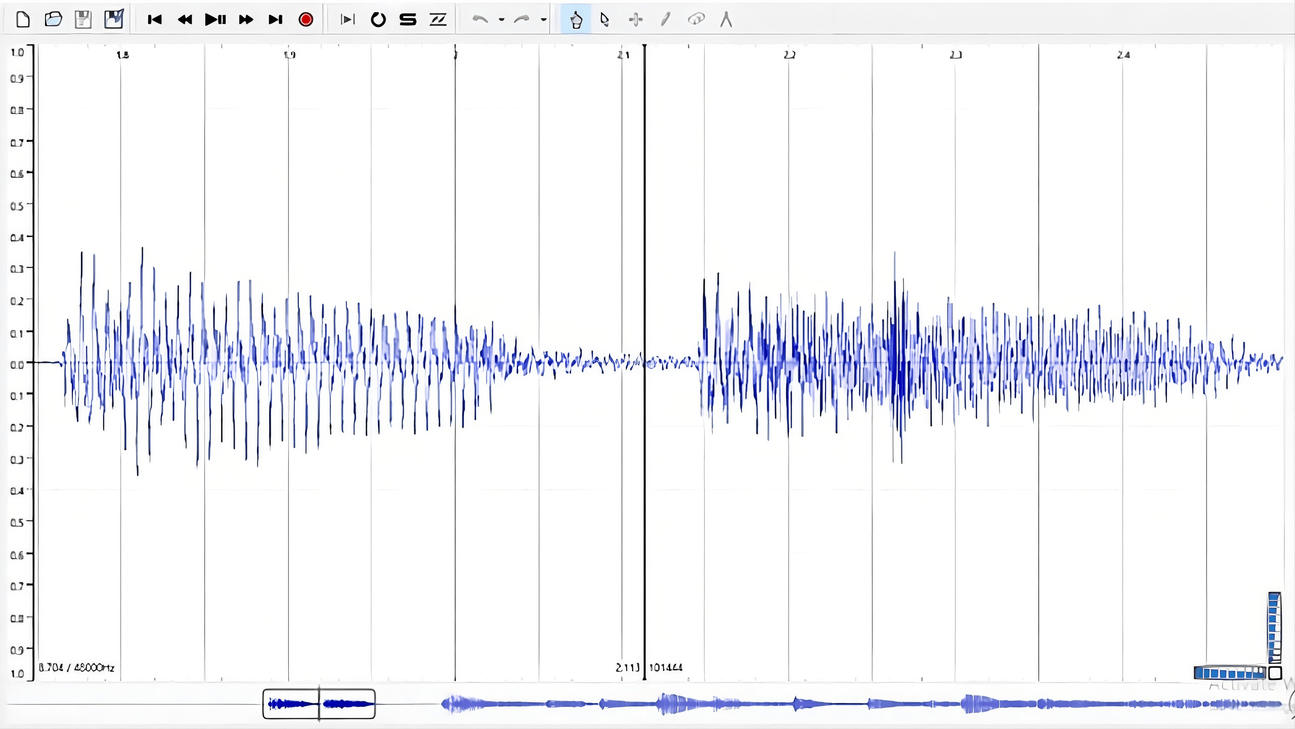
Figure 2 | Visualization of the first two notes from the performance recordings (36th trial), depicted using Sonic Visualiser.
The Note Onset Detector tool in the Transform window of Sonic Visualiser was used to determine the exact timing of each note (approximate error in automatic onset detection is ±5–15 ms). As the peaks indicate the striking of the strings, these moments were highlighted by additional vertical lines, showing the exact millisecond when the note was played. All note timing was manually curated to get rid of spurious background noise. In more detail, Sonic Visualiser indicated some background sounds as additional notes, so while transferring obtained data, these wrong onsets were deleted from results. Eleven precise note times were recorded in each trial, resulting in the quantification of 10 intervals.
During practice, some trials contained mistakes, such as playing an extra note or skipping a note. Prior to data analysis, these errors were defined as incorrect sequences of notes. Trials with mistakes were stopped at the point of error and therefore did not include all 11 notes. These incomplete trials were removed from the dataset and were not considered in subsequent analyses, as they would disrupt overall trends. In total, 11 trials contained mistakes, reducing the dataset from 55 to 44 trials. The removal of these trials was intended to reduce distortions in interval-based analyses and accurately capture learning trends, as including incomplete or error-containing sequences would disrupt the evaluation of interval timing and the progression of skill acquisition.
The time period of practice sessions was not considered at the start. Overall, the first eight trials(three warm-up trials and the first five recorded trials), the next twenty trials (from the 6th to the 25th recorded trial, inclusive), and the last twenty-nine trials (from the 26th to the 55th trial, inclusive) were recorded separately on different days. There was a 10-day gap between the first and second practice sessions and a 13-day gap between the second and third sessions. In total, the experiment was conducted over a period of 23 days. However, no additional analyses or statistical comparisons were performed based on these time gaps.
Data analysis
To prepare the dataset for analysis, all timing data was organized systematically in Google Sheets. To compare the results across trials, the experiment focused on calculating the intervals between notes for each trial. Accounting for the fact that the performance did not start exactly at the moment of each recording, the first notes’ onsets of each trial were subtracted from all subsequent notes to normalize the timing relative to zero. This procedure served only to align trials to a common starting point and did not affect the relative timing between notes. Next, intervals were calculated as the difference in time between consecutive notes. With 11 notes in each trial, this resulted in 10 intervals per trial and the total dataset of 440 intervals across all trials. Therefore, the subtraction of first notes’ onsets was only related to recording offsets and did not distort interval dynamics within trials. Using these intervals, statistical analyses were then conducted, including estimations of mean, standard deviation, and coefficient of variation for each interval number across trials. This approach allowed systematic comparison of the data and identification patterns in performance as a function of practice.
Results
The duration of the melody decreased with practice.
To quantify improvement in timing consistency as a function of practice, the entire duration of each trial with 11 notes (10 intervals) was calculated.
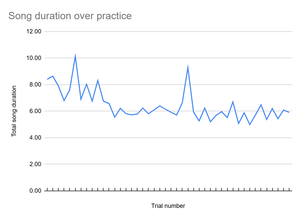
To test how the duration of the song changed with practice, I added up all 10 intervals per trial to compute its total duration, and then plotted the total duration as a function of trial number (Fig. 3). Note that the duration of the song gradually decreases with practice, suggesting increased proficiency. Trials 6 and 34 were outliers in this trend; relistening to these trials revealed long single intervals. Additionally, a vivid reduction in duration occurred after the 17th trial, suggesting that approximately this amount of practice might be enough to improve timing skills.
Trial to trial variability decreased with practice.
To compute the variability across successive trials, I computed the absolute value of the difference between intervals of all of the adjacent pairs (Fig. 4). For instance, the differences between intervals of first and second trials, then between seconds and third trials, and so on. It resulted in 43 columns of differences in intervals. Then the median of each column was indicated. If each interval was identical across trials, then this analysis would show zero difference. On the other hand, if intervals were inconsistent and consistently differed across successive trials, then this value would be high. Overall, this analysis estimated the similarity between two successive trials. As shown in Figure 4, over practice successive trials became more similar to each other, reflecting more consistent interval timing.
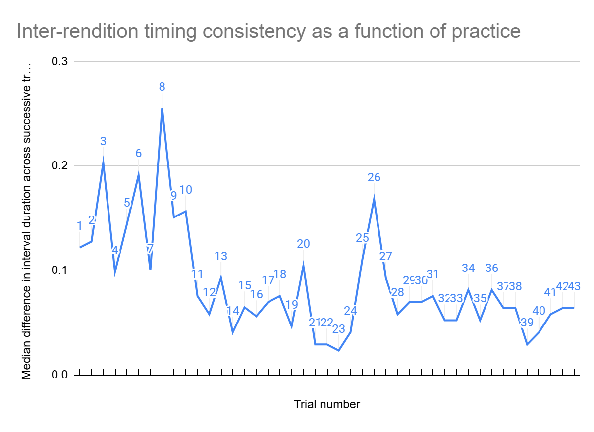
As the line generally follows a downward trajectory, this suggests that variation between trial intervals decreases with practice. Being more precise, the plot suggests that at the start, for about 10 median values of successful trial pairs differences, timing remained variable. After that, with continued practice, the intertrial variability decreased, with the median value never becoming more than 0.1, except for one extraordinary pattern (26th pair, due to delay in one of adjacent trials – 34), which directly shows that consistency would increase with practice.
Empirical support for subjective performance assessment.
To test whether my subjective sense of performance quality had quantitative support, I made a personal note during my practice history of which two trials I considered very well performed and closest to my desired target.I identified two exact trials – 41 and 44 – which I named ‘target song 1’ and ‘target song 2’. If my subjective sense of performance quality is accurate, then these songs should exhibit more precise timing in their execution than two randomly selected trials.Alternatively, if my subjective sense of quality is meaningless, then these two target songs would display similar performance metrics (e.g., note consistency) as any other songs in my dataset.
Therefore, several methods were used to find an answer, with the results shown in Figures 5 and 6.
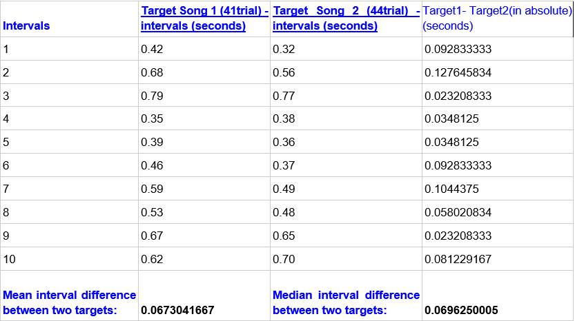
As a first observation, looking at Figure 5, it could be noted that the median difference between the target songs is also less than 0.1, as in most pairs of trials (Fig. 4). While this suggests that their timing is very close to each other, as anticipated, there are numerous other trial differences across the dataset that do not vary much more.
Figure 4 directly only compares the difference between aligned intervals in adjacent trials. So, I wondered about the full range of intervals across all notes and all songs. To visualize this, I constructed a histogram of all differences between all intervals in the dataset (pairwise differences) (Fig. 6).
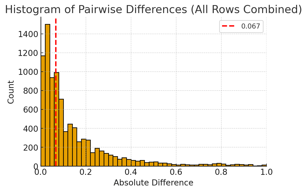
Figure 6 shows the full range of intervals, and the dashed red line indicates the median interval of the differences between target songs 1 and 2. The target songs indeed were on the low end of the distribution of inter-interval consistency. However, they cannot be considered as a perfect match, as there are many other differences that are even smaller.
Target songs (41 and 44th trial) were more closely related to the final trial, rather than first.
To test if the two target songs were more alike than the first and last trials of the dataset, two plots were created (Figures 7 and 8). The durations of the target 1 (41st) and target 2 (44th) trials were subtracted from the interval durations of the first and last attempts, in order to obtain time differences between the same intervals (Figure 7). This provides the information on patterns of changes happening during practice.
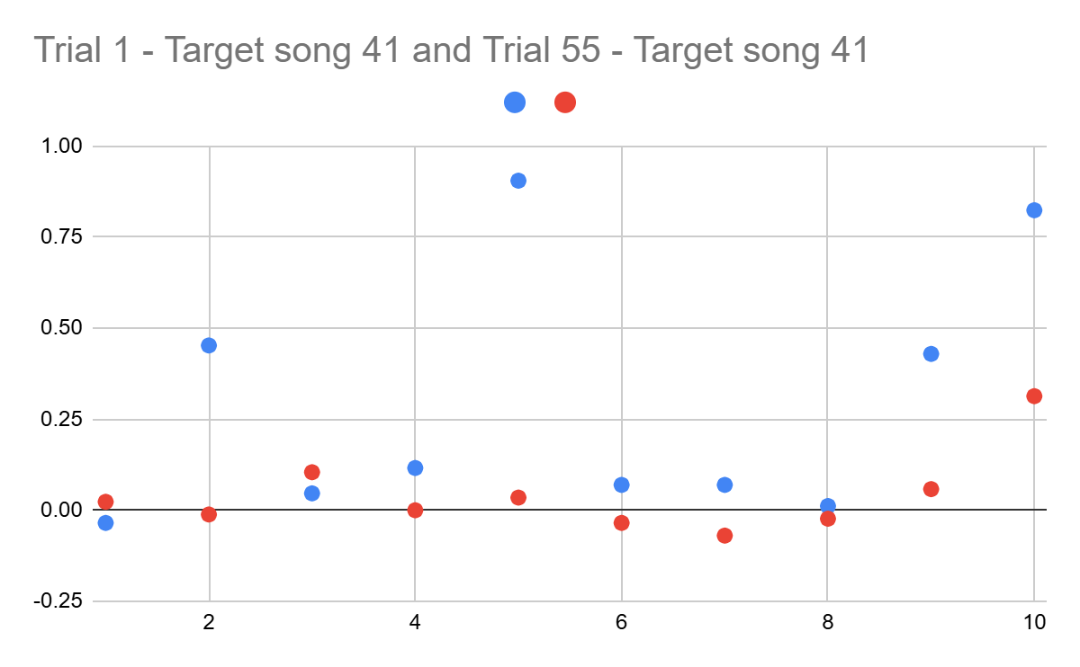
Analyzing this plot, it could be observed that the differences from the first trial are mostly positive, while the last trial includes mostly negative values, with only a few positive points. Since the last trial shows a shorter duration than the 41st trial, and the first trial was almost always longer than the 41st interval’s duration, this suggests that, through practice, the speed of playing the melody has substantially increased.
To support this conclusion, the same calculations were made using the 44th (other target song) indicators (Figure 8).
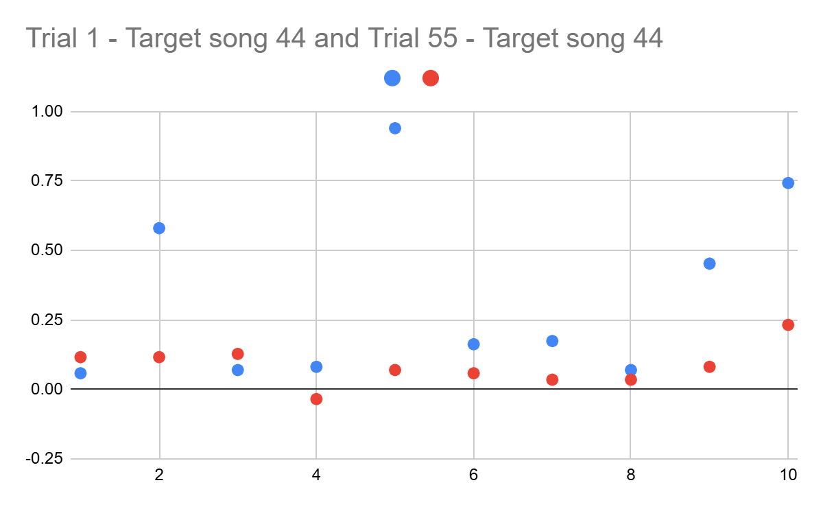
Although there are no more negative values in the differences of 44 trials and the last trial, the results still vary a lot, supporting the previous suggestion. Moreover, red dots are almost always closer to zero than the blue ones, meaning that the last trial was more consistently played overall.
However, additional observations can be made. The differences of the first intervals for both examples do not show a similar pattern, being larger or smaller regardless of the trial number. This suggests that this note was one of the easiest parts to follow in timing. Furthermore, the differences between 3, 4, 8 intervals for both datasets follow the identified pattern, but vary less than for 0.1 seconds, provoking the thought that these parts were also among the easiest parts to play consistently.
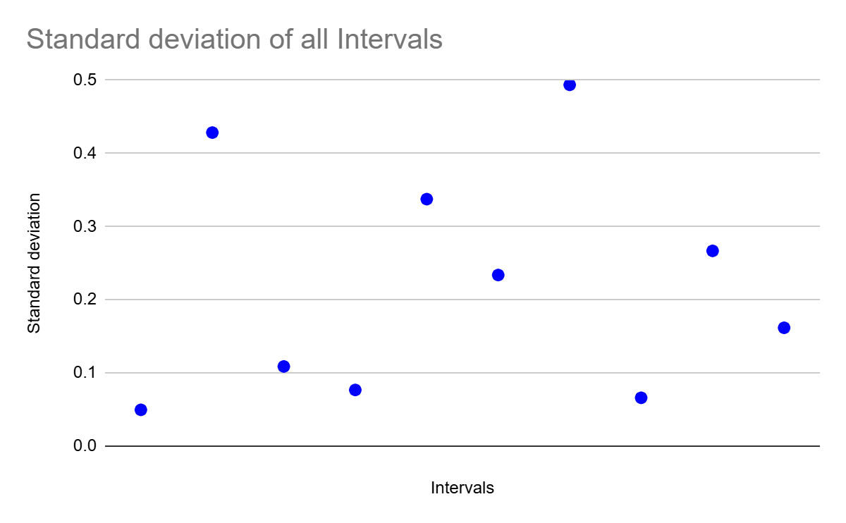
Variability within trials did not increase as the song progressed.
To test if interval consistency within a trial depended on how far into the song was played, the standard deviation for the 10 intervals across the whole dataset was calculated. Although it might be expected that the intervals would become more variable as the melody progresses, Figure 9 clearly showed no trend in interval timing consistency within the song.
Trial to trial variability in interval timing decreased with practice
To test if variability reduced with practice, I computed the C.V. of all aligned interval differences for every set of 10 trials within an interval, using a specific formula (C.V.(i:i+10)) (Figure 10). For example, if there are intervals of 20 trials on the whole, the standard deviation is not obtained for just two groups of trials (1–10 and 11–20), but for 11 groups (1–10, 2–12, 3–13, …, 11–20). Only the median value of C.V. for each column was considered, resulting in 35 figures of median C.V. Note that figure 4 analyzed adjacent differences, detecting trial-to-trial consistency, this analysis, using S.D. and C.V. for every pair of 10 trials, capture entire performance trends.
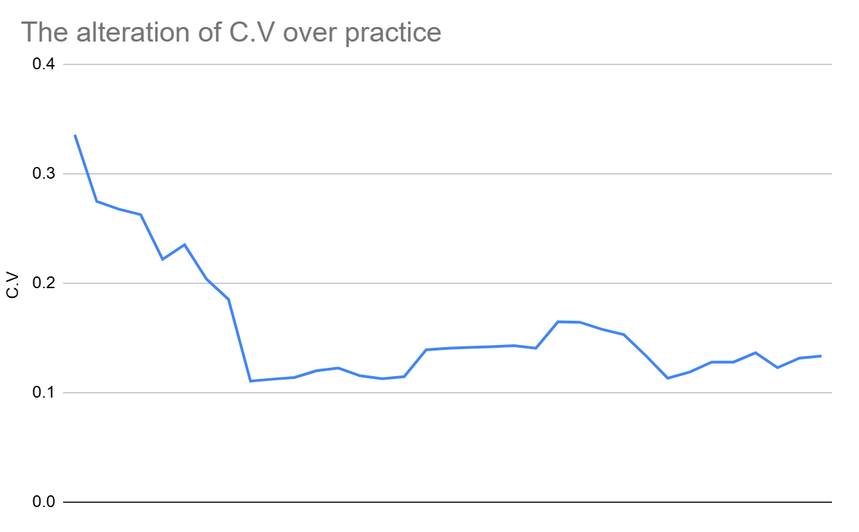
Figure 10 shows that C.V. followed a decreasing trend throughout the trial recordings. Additionally, it could be highlighted that approximately 20 trials were enough to obtain the stable timing consistency in performances, which was also already observed earlier.
Conclusion
The purpose of this study was to bring quantitative rigor to the assessment of musician performance. In this paper, I used six different and independent analyses to examine how performance changed with practice. The results demonstrated a general reduction in timing variability and increased consistency, suggesting that repeated practice contributes to the stabilization and refinement of motor performance. However, the results should be interpreted within the limitations of the study design.
Limitations
This is a self-made experiment, being considered as a case study. So, a number of limitations that appeared during the experiment should be mentioned. First of all, the single participant design inhibits the generalization of results and restricts conclusions to descriptive within-subject dynamics. Moreover, the participant’s past experience of playing the guitar introduced bias toward the obtained results, since the participant was more likely to quickly take the concepts of the new melody in comparison to a person without any experience. Practice sessions were self-directed and uncontrolled, which may have affected the overall results as an additional factor influencing the overall skill acquisition.
Some trials containing performance errors were excluded from the dataset (reducing the number of trials from 55 to 44) to ensure accurate assessment of interval timing and learning trends. Despite it being a necessary step, this represents a limitation because it reduces the sample size and may slightly restrict the ability to capture the full spectrum of learning dynamics.
Another limitation was the manual correction of additional onsets that the program added due to background noise. As it was only checked and rechecked by 2 people, it may introduce subjectivity. Additionally, multiple statistical comparisons were conducted without applying a correction for multiple testing, such as Bonferroni corrections, which reduces the reliability of the results. Finally, no neural or reward-related measurements were included, and therefore, neurobiological interpretations remain speculative.
Future directions
In the future, the progress and refinement of the research could be achieved by augmenting the number of participants in the experiment. This would allow for more robust statistical analysis and greater generalizability of the findings. Additionally, applying corrections for multiple comparisons, such as the Bonferroni method, would strengthen the reliability of the results.
The usage of neuroimaging techniques (fMRI or PET) may enable us to observe some neural mechanisms, underlying motor learning and help to link the results of experiments with biological processes.
Summary
Although this study does not include neural measurements or experimental manipulation of reward, the observed reduction in timing variability across repeated practice is consistent with established behavioral models of motor learning. Previous research suggests that variability reduction and movement stabilization are supported by interactions between the cerebellum, motor cortex, and basal ganglia, particularly through internal predictive models of timing. Therefore, while no direct conclusions about dopaminergic mechanisms can be drawn from the present data, the behavioral dynamics observed here align with theoretical frameworks describing gradual optimization of motor timing through practice.
References
- Zador, A. M. (2019). A critique of pure learning and what artificial neural networks can learn from animal brains. Nature Communications, 10(1), 3770. https://www.nature.com/articles/s41467-019-11786-6 [↩]
- Schmidt, R. A., & Lee, T. D. (1999). Motor control and learning: A behavioral emphasis (3rd ed.). Human Kinetics. [↩]
- Shmuelof, L., & Krakauer, J. W. (2011). Are we ready for a natural history of motor learning? Neuron, 72(3), 469–476. https://doi.org/10.1016/j.neuron.2011.10.017 [↩]
- Sternad, D. (2018). It’s not (only) the mean that matters: Variability, noise and exploration in skill learning. Current Opinion in Behavioral Sciences, 20, 183–195. https://doi.org/10.1016/j.cobeha.2018.01.004 [↩]
- Wu, H. G., Miyamoto, Y. R., Castro, L. N. G., Ölveczky, B. P., & Smith, M. A. (2014). Temporal structure of motor variability is dynamically regulated and predicts motor learning ability. Nature Neuroscience, 17(2), 312–321. https://doi.org/10.1038/nn.3616 [↩]
- Ölveczky, B. P., Andalman, A. S., & Fee, M. S. (2005). Vocal experimentation in the juvenile songbird requires a basal ganglia circuit. PLoS Biology, 3(5), e153. https://doi.org/10.1371/journal.pbio.0030153 [↩]
- Brainard, M. S., & Doupe, A. J. (2002). What songbirds teach us about learning. Nature, 417(6886), 351–358. https://doi.org/10.1038/417351a [↩]
- Finney, S. A. (1997). Auditory feedback and musical keyboard performance. Music Perception, 15(2), 153–174.https://doi.org/10.2307/40285747 [↩]
- Montague, P. R., Dayan, P., & Schultz, W. (1997). A neural substrate of prediction and reward. Science, 275(5306), 1593–1599. https://doi.org/10.1126/science.275.5306.1593 [↩] [↩]
- Otani, S., Daniel, H., Roisin, M.-P., & Crepel, F. (2003). Dopaminergic modulation of long-term synaptic plasticity in rat prefrontal neurons. Cerebral Cortex, 13(11), 1251–1256.https://doi.org/10.1093/cercor/bhg092 [↩]
- Gadagkar, V., Puzerey, P. A., Chen, R., Baird-Daniel, E., Farhang, A. R., & Goldberg, J. H. (2016). Dopamine neurons encode performance error in singing birds. Science, 354(6317), 1278–1282. https://doi.org/10.1126/science.aah6837 [↩] [↩]
- Repp, B. H. (2005). Sensorimotor synchronization: A review of the tapping literature. Psychonomic Bulletin & Review, 12(6), 969–992. https://doi.org/10.3758/BF03206433 [↩]
- Drake, C., & Palmer, C. (2000). Skill acquisition in music performance: Relations between planning and temporal control. Cognition, 74(1), 1–32. https://doi.org/10.1016/S0010-0277(99)00061-X [↩]
- Paton, J. J., & Buonomano, D. V. (2018). The neural basis of timing: Distributed mechanisms for diverse functions. Neuron, 98(4), 687–705. https://www.cell.com/neuron/fulltext/S0896-62731830251-4 [↩] [↩]
- Teki, S., Grube, M., Kumar, S., & Griffiths, T. D. (2011). Distinct neural substrates of duration-based and beat-based auditory timing. Journal of Neuroscience, 31(10), 3805–3812.https://doi.org/10.1523/JNEUROSCI.5561-10.2011 [↩]
- Ivry, R. B., & Spencer, R. M. C. (2004). The neural representation of time. Current Opinion in Neurobiology, 14(2), 225–232. https://doi.org/10.1016/j.conb.2004.03.013 [↩]
- Ito, M. (2008). Control of mental activities by internal models in the cerebellum. Nature Reviews Neuroscience, 9(4), 304–313. https://doi.org/10.1038/nrn2332 [↩]


 and a Developing (India) Economy")