Deep Neural Networks for Breast Cancer Ultrasound Classification and Segmentation in Data-Constrained Settings: An Exploratory Study

Veer Chowdhary¹, Mitchell T. Dennis^2
1 The Nueva School, 131 E 28th Avenue, San Mateo, CA 94403
² Institute for Astronomy, University of Hawai‘i at Ma̅noa, 2680 Woodlawn Drive, Honolulu, HI 96816

Abstract

Breast cancer diagnosis using ultrasound imaging remains a major challenge in the US. Though the images themselves are objective, radiologist interpretation, access to specialists, and access to high quality equipment make it difficult to ensure consistent diagnostic accuracy across all settings. These challenges are especially pronounced in underrepresented or smaller patient populations, where collecting large, diverse, and well-annotated datasets is less feasible. As a result, it is important to understand whether or not deep learning models can attain meaningful performance under constrained data settings. In this paper, we explore the use of deep neural networks for breast cancer diagnostic classification and image segmentation using a limited dataset of breast ultrasounds. For this study, we used the USG-BrEaST-Lesions dataset, which consists of 256 images, and includes radiologist annotations, as well as the associated clinical data. We trained a series of machine learning algorithms to evaluate the best performing model in each of three categories: simple feature based classification using only tabular data, an image only classification using convolutional neural networks, a multi-modal image-feature classification using either fused neural networks or weighted voting depending on the tabular component, and an image segmentation neural network to identify tumors instead of classifying them as benign or malignant. The results show that deep learning has some promise in data-constrained settings, but performance is uneven and heavily dependent on the type of data used. The strongest classification result was a 0.97 receiver operator characteristic area under the curve (ROC AUC), but this appears to be driven mainly by the tabular data, and because it is a single estimate, it should be interpreted cautiously. The tabular-only models performed reasonably despite using only two features, though that also limits their practical predictive value. The image-only models performed notably worse, with a best ROC AUC of 0.70, suggesting the ultrasound images alone were not sufficient to reliably distinguish benign from malignant tumors in this dataset. The multimodal models also did not meaningfully outperform their individual components, possibly due to integration or generalization challenges. Overall, these results should be interpreted as exploratory findings that demonstrate the promise of utilizing deep learning models under constrained data settings rather than as evidence of readiness for autonomous clinical deployment. Although the models achieved reasonable performance within the scope of this dataset, these findings should not be interpreted as evidence of current clinical possibility, but rather as an initial investigation into the feasibility and limitations of deep learning approaches in small-data medical settings.

Keywords: breast cancer, deep learning, ultrasound imaging, convolutional neural networks, medical image segmentation, machine learning, small data learning, diagnostic accuracy

Introduction

Breast cancer is the most prevalent cancer in the world and remains the major cause of cancer-associated deaths globally. Based on estimates from GLOBCAN 2020, breast cancer has surpassed lung cancer as the most commonly diagnosed cancer, with an estimated 2.3 million women diagnosed with breast cancer and 685,000 breast cancer associated deaths worldwide¹. A quick and accurate diagnosis is extremely important to improve patient results, as early treatment greatly increases survival rates and reduces the use of intensive and invasive treatments. Although medical technology has greatly improved, challenges persist in the detection phase, notably diagnostic accuracy, time, and patient comfort. Breast cancer is generally diagnosed through mammography and ultrasounds. Mammography (MAM), while effective in older women, has limited benefit for younger women, has shown to have reduced accuracy in dense breasts, and is often inaccessible in low-resource settings due to high costs. Compared to MAM, ultrasound (US), is low-cost, radiation-free, portable, and available. However, US scans are less reliable and consistent because their accuracy depends heavily on the skill and experience of the radiologist performing them^2,3. Complicating matters further, in many regions, both in resource constrained countries and even in America, access to mammography machines remains a significant challenge^4,5,6. Conversely, while ultrasound machines are more accessible, access to experienced technicians to evaluate them for breast cancer are worse than for mammography machines⁷. Despite this, ultrasounds have the potential to help bridge this gap by supplementing existing resources and providing access to care in areas where resources are extremely limited⁸, and machine learning can be one avenue to improving access.

Breast cancer is generally diagnosed through mammography and ultrasound imaging with more conclusive follow up diagnostic tools like biopsies. Mammography is generally more effective in older women^9,10, but sensitivity can drop significantly in low density tissue (up to 48% in the densest tissue)^11,12. Ultrasounds offer lower cost, radiation-free alternatives that are also more portable and can be sensitive to tumors in more dense breast tissue¹³. However, the accuracy of ultrasounds are highly skill dependent relying heavily on the radiologist performance¹⁴, which can be far from uniform across practitioners but can benefit from the use of artificial intelligence to reduce false positives¹⁵. These findings motivate the exploration of deep learning (DL) approaches that can provide a more consistent diagnosis that is less clinician dependent.

DL is highly effective at image-related tasks, including abnormalities detection, segmentation, and classification and offers promise as a tool that can address the diagnostic challenges such as operator-dependent variability. Its promise has been the subject of substantial research over the past decade. Deep neural networks (DNNs), particularly convolutional neural networks (CNNs), are well suited to the analysis of medical images due to their unique ability to learn spatial features from image data without hand crafted feature engineering¹⁶. Turning to breast ultrasounds in particular,¹⁷ provides a comprehensive review of several studies concluding that DL is highly promising in reducing operator dependence in breast ultrasound diagnostics.

Additionally,¹⁵ trained a large DL system on more than ∼288, 000 ultrasound exam, achieving a higher receiver operator characteristic area under the curve (ROC AUC) score than 10 board certified radiologists (0.962 to 0.924 ± 0.02), reduced false positives by nearly ∼37% and reducing biopsy requests by ∼ 8%. This is in agreement with other studies which show improved specificity (∼40%) for computer aided diagnostics (CAD)¹⁴, and a higher ROC AUC score for DL when compared to inexperienced radiologists but similar scores for experienced ones¹⁸. Significant debate still exists with some studies suggesting that DL based interpretation of Breast US can match or even exceed the accuracy of human radiologists^{15,17,19,20,21} and others showing lower sensitivity than human radiologists^{14,18,22,23,24}.

While these studies mostly focus on diagnosing breast cancer, others have employed DL to identify tumors from scans using image segmentation^25,26,27. U-Net architectures have become the dominant approach in this field.²⁶ demonstrated that U-Net variants can achieve high performance (Dice score ∼ 0.9) on small datasets (∼500 images) and²⁵ achieved Dice scores of 0.87 and 0.76 on datasets of 562 and 163 images, respectively. These works demonstrate the viability of training these types of networks using small datasets.

The most reliable DL systems are trained on thousands or even hundreds of thousands of images are still limited by the scope of their data, i.e. if a demographic or group is not sufficiently represented in their training data, extending those models’ results to that group is more challenging. Therefore, exploring the development of whether or not effective DL algorithms can be trained from smaller datasets—which are more feasible to collect in many under-served and lower-resource environments—remains a pressing question in breast cancer research.

This paper takes an exploratory approach to see whether strong diagnostic accuracy can still be achieved with a relatively small dataset. Instead of trying to compete with large-scale models, it focuses on understanding what’s realistically possible when data is limited. The goal is to reflect real-world situations especially in settings where large, well-structured datasets aren’t easily available and to explore whether useful performance can still be reached under those constraints. This study is not intended to develop an immediately deployable diagnostic system to hospitals, but rather to investigate the feasibility and limitations of deep learning in data-constrained settings. Specifically, we ask: 1. Can deep learning models achieve meaningful performance for breast cancer classification and segmentation when trained on a constrained dataset. 2. In settings of constrained data, how do image-only, tabular-only, and combined approaches compare in their ability to support diagnostic accuracy.

Methods

This section has 4 subsections: Data Selection, Data Preparation, and Network Design and Implementation.

Data Selection

One of the most important steps while processing the data is dataset selection and cleaning to make it more efficient. This includes the exclusion of certain categories as well as data segregation. The model used the USG-BrEaST-Lesions-Dataset²⁸ as input. The dataset contains 256 breast ultrasound images classified into three different groups: 154 benign lesions, 98 malignant lesions, and 4 normal breast tissue scans. Each image in the dataset is annotated by a radiologist for tumor borders. Each scan is also assigned Breast Imaging-Reporting and Data System (BI-RADS)²⁹ scores, a standardized system to classify breast lesion risk based on imaging features.

Of the columns presented in the dataset, nearly all of them relied, in whole or in part, on the expertise of the accompanying ultra-sound technician. These column features were then combined to form the BI-RADS score which evaluates the likelihood of breast cancer. These can produce leakage in our models resulting in over-optimistic model performance. We therefore excluded all columns within our dataset except for ‘Age’, ‘Signs’, and ‘Symptoms’ which are all reported by either the patient or a clinician before the ultrasound is conducted. The images used to train the model were the ultrasound scans, as well as their accompanying masks, where a radiologist has marked the tumor. Both the ultrasound scans and the masks are 3-channel images with 8 bits per channel. While ultrasounds inherently produce single-channel, grayscale images, these are typically exported to DICOM files; whereas the files provided by this dataset are PNG files. Therefore we presume the curators of the dataset converted the images to PNG files which by default are 3 channels. The channels in each of our files are redundant replications of the same grayscale intensity across the R, G, and B channels used by PNG. For our machine learning models, we use single channel grayscale images where able, and 3 channels when in the case a prebuilt model requires it.

Data Preparation

The ‘Symptoms’ column is missing a significant amount of data (∼37%) which are too many missing points to justify including in the dataset via one-hot-encoding, even with a designated ‘missing data’ value, and therefore it also ended up being excluded. The ‘Signs’ column is also missing some data (∼18%), but this is a more manageable number than for the ‘Symptoms’ column. We one-hot-encoded the different values in the ‘Sign’ column, keeping the missing entries as a distinct column. Furthermore, in the ‘Age’ column, there were some missing values marked as “not available” which were replaced with the median of the available data. We kept this column even with missing values because we considered age to be an important indicator for diagnosis and there were not so many missing values that replacing them with the median age value significantly affected the overall distribution. Finally, the ‘Classification’ column, which had labels of benign, malignant, and normal, was mapped to numerical values (0, 1, and 2, respectively), with cases of type “normal” excluded because there were only four samples, making it impossible to train a reliable model on this category due to the limited available data.

The class totals within the 252 images remaining images were 154 benign and 98 malignant tumors. Because of this roughly 3:2 imbalance, we implemented weighting where possible within the training for each model. The weights were set using the following formula

(1)  

given class, 𝑛_total is the total number of data points, 𝑛_classes is the total number of classes, and 𝑛_𝑐 is the number of data points in the given class. Using this formula we got values of 0.818 and 1.286. Because XGBoost and CatBoost use slightly different parameters in their libraries, we simply adopt a single weight ratio of 154/98 which achieves the same effect. As described below, we used K-Fold cross validation when training our models, therefore the weights are updated for the individual stratified data splits. These should not be significantly different from the global weights.

Our data was split according to the following prescription. A master data split with an 80%, 10%, 10% split across training, validation, and testing dataset. This split is only used for three specific purposes: the final saved models (ensuring consistent testing across all of our different values), optimizing our voting pairs described below, and providing the single seed point estimates for the final deep neural network and convolutional neural network models. In addition to this split, we utilize a nested cross-validation scheme using stratified K-Folds (stratified ensures we maintain the same class ratios) so that we can obtain distributions of our metrics and obtain confidence intervals on our results. This is done with 5 splits of 80% training/20% testing repeated a total of 10 times for each K-Fold yielding 50 total metric evaluations for each model type. For the DNN and CNN, validation data is created from the training data to provide validation losses which will be necessary for the callback conditions which we describe later.

Specific image network considerations:

We standardize all images across all models to a size of 128×128 pixels, and transform their pixel values from standard 24 bit RGB values to [-1, 1] in each image channel (or single channel for the grayscale network). This is done for both the classification models and our segmentation models. The transformation is necessary to make the images work with the MobileNetV2 algorithm³⁰ which we used as one component in some of our image algorithms. Additionally, the image classification networks utilize only the raw ultra-sound images whereas the segmentation networks utilize both raw ultra-sound images and their accompanying tumor masks.

Network Design and Implementation

We trained a series of machine learning algorithms to evaluate the best performing model in each of three categories. These were: simple feature based classification using only tabular data, an image only classification using convolutional neural networks, a multi-modal image-feature classification using either fused neural networks or weighted voting depending on the tabular component, and an image segmentation neural network to identify tumors instead of classifying them as benign or malignant.

Tabular-Only Classification Algorithm

For our tabular data, we used a series of different algorithms including logistic regression, random forest, extreme gradient boosting, light gradient boosting, categorical boosting, and a tabular neural network. These models were all built to perform a simple binary classification of benign or malignant using only the clinical tabular data provided with the breast ultrasound images. This model, unlike other networks, did not include any imaging data whatsoever. Because we only utilize two columns for these models, we do not expect these to perform significantly better than simply assigning a single value to all cases which would achieve a success rate of approximately 61%. Additionally, because there is some inherent randomness to many of these methods and to how the data is split, we implement K-Fold cross validation to evaluate the distribution of possible results. For each method we implement 5 folds, repeated 10 times each for a total of 50 results for each method.

For our deep neural network, we investigated which architecture best suits our data. To do this we also use K-Fold splitting (50 total folds as above) and use these splits to select the best architecture from three different base models. The folds were tested across different hidden unit dimensions and dropout rates. The resulting best model was then treated to another 50 K-folds as above to evaluate its distribution of model performance across a single architecture. Consistent across architectures are an initial Batch Normalization layer, followed by Dense/Dropout layer pairs, and finally a single Dense output layer with a Sigmoid activation. We use a relatively small/shallow network as our dataset is small and therefore the risk of overfitting with large numbers of parameters is high³¹. We keep to the recommendations of³² with a lower bound of roughly 10-28 hidden units for our 14 features (the one-hot-encoded ‘Signs’ produced 13 columns) and deliberately probe as high as 64 hidden units. The number of hidden units at each consecutive layer is reduced by a factor of 2, a typical decision, motivating our choice of only 2 hidden layers. Any more layers would result in hidden layers with very few units that would not contribute significantly to the model. The DNNs were trained using categorical cross-entropy loss, an Adam optimizer³³ with a learning rate of 0.001, a plateau monitor — which adjusted the models learning rate if the model stopped improving — and an early stopping condition to halt the training once the model was no longer improving that only triggers after the plateau monitor adjusted the learning rate. The model performance was tracked over 50 epochs. A summary table of the network architecture is included as Table 1.

Number	Type	Neurons/ Rate	Activation Function
1	Input	14	Linear
2	Batch Norm.	N/A	N/A
3	Dense	32	ReLU
4	Dropout	0.2	N/A
5	Dense	16	ReLU
4	Dropout	0.2	N/A
13	Dense	1	Sigmoid

Even though we are only able to evaluate on 2 data columns, limiting the predictive power of our models, we perform this exercise to see the distinction between the value provided by both tabular and image data, and the value of meaningfully combining them to achieve greater accuracy. 

Image-Only Classification Neural Network

We follow the same scheme as before using K-Fold cross validation to determine the most effective architecture and data augmentation choices. The augmentations are simple image transformations performed on the training images to create pseudo-unique samples to artificially increase the size of the training data³⁵. We again use cross validation to test varying levels of data augmentation in our attempt to combat overfitting to our small dataset using methods that previous breast ultra sound studies have used including random horizontal flip rotation, translation, zoom, and sheer^36,37,38. The levels we test range from no augmentation to “aggressive’ augmentation and are well described by the values provided in Table 6. This table, found in our results section, also includes ROC AUC scores and their confidence intervals. This test was only performed on our custom grayscale CNN and from it we selected the best performing augmentation to use for all of our image networks including the multi-modal neural networks and the image segmentation network.

Similar to the tabular models, we also evaluated three different kinds of image models to deter-mine which was the most effective at classifying the ultrasound images. These three architecture types were MobileNetV2³⁹ with weights trained on ‘ImageNet’⁴⁰, MobileNetV2 from scratch (both requiring 3 image channels), and a custom convolutional neural network using grayscale images.

Our custom CNN is built with 3, 3-layer units comprised of a 2D convolution layer followed by batch normalization and max pooling. These are then fed through a global average pooling layer and output in a single sigmoid layer. On the input side of our CNNs, We use a VGGNet design principle, doubling the number of filters per block using only a small number of blocks to reduce the risk for over fitting^41,31. Our choice of 3×3 convolutions, batch normalization, and global average pooling as well as dropout for regularization are well documented as best practice within the existing literature^42,43,44,45. A table describing the architecture of the CNN is provided as Table 2.

Layer	Output shape	Parameters	Trainable
Input	128 × 128 × 1	—	—
Conv2D, 32 filters, 3×3, ReLU	128 × 128 × 32	320	320
BatchNormalization	128 × 128 × 32	128	64
MaxPooling2D, 2×2	64 × 64 × 32	0	0
Conv2D, 64 filters, 3×3, ReLU	64 × 64 × 64	18,496	18,496
BatchNormalization	64 × 64 × 64	256	128
MaxPooling2D, 2×2	32 × 32 × 64	0	0
Conv2D, 128 filters, 3×3, ReLU	32 × 32 × 128	73,856	73,856
BatchNormalization	32 × 32 × 128	512	256
GlobalAveragePooling2D	128	0	0
Dropout (rate = 0.3)	128	0	0
Dense, 1 unit, sigmoid	1	129	129

We also implement MobileNetV2 as it has been shown to be effective at diagnosing cancer using ultra-sound images⁴⁶. With so little data, it is likely that MobileNet, pretrained on other image and fine-tuned with our ultra-sound images, will be more successful than attempting to train networks from scratch and has been used to diagnose breast cancer from ultra sounds in other studies. MobileNetV2’s unique structure, inverted residuals with linear bottlenecks, helps it be both accurate and computationally efficient as it is good for mobile or resource-limited devices.

Like the previous model, these networks were also training with sparse categorical cross-entropy loss, an Adam optimizer with learning rate of 0.001, a plateau monitor, and an early stopping condition. However, unlike our other networks whose weights are trained from scratch, the MobileNetV2 with ‘ImageNet’ weights had to be trained in two stages. The first stage only trains the custom dropout and output layers we added to the inference stage, and does not train any of the weights in the MobileNet layers. This is to preserve the filters learned by MobileNet in its original training on ‘ImageNet’. Once this first pass through training is completed, the last 30 layers of the model are unfrozen, and training begun again with a smaller learning rate (0.00001). This allows MobileNet to interface well with the new layers we added, while still preserving the majority of its pretrained weights. A summary of the network and its architecture can be found in ⁴⁶.

Image and Tabular Classification Neural Network

Last among our classification tasks, we combine the various tabular data models with the most effective image model to maximize the accuracy of our classification task. For models that cannot integrate directly to the CNNs (i.e. they are not neural networks), we combine the results through the use of weighted voting where each model in a tabular-CNN pair gives a prediction on a set of input data, and that prediction is weighted to maximize the area under the curve in the receiver-operator-characteristic curve. The weights for the two models must sum to 1, and so the weight of the tabular model is the complement of the image model.

For the neural networks, the models were combined by removing the inference layer of both and concatenating the second to last layers of the previous two models. Similar to the fine-tuning of the MobileNetv2 with ‘ImageNet’ weights above, we then fine-tuned by training again with a small learning rate so that each models features and errors could back-propagate to both model components. By combining both image and tabular data, the model can use both cues from the images and diagnostic information from the clinical data, which could improve accuracy. After the concatenation, we also attached additonal Dense/Dropout layer pairs. Doing this allows the combined network to weigh the features from both the tabular and image classifiers and use all available information to evaluate the testing data.

Image-to-Mask Segmentation Neural Network

The final network is for segmentation of images, specifically tumor detection in images of breast ultrasounds. This model is fundamentally different from the ones above. While those gave a single output, this network processes the ultrasound image, extracts its features through convolutions and then recreates the tumor masks in the size of the original image. To do this, it employs a U-Net architecture, first proposed by⁴⁷ for biomedical image segmentation, with MobileNetV2 used again as an encoder, but with the weights frozen entirely during training³⁹. The use of a U-Net architecture with a MobileNetV2 encoder for the segmentation task was motivated by previous research showing the effectiveness of the former with respect to breast ultrasound image segmentation⁴⁸. The U-Net architecture first transforms the images using the convolutional layers of MobileNet, and then utilizes reconstruction layers in order to create the segmented output that forms the mask that highlights the area of the tumor in the image. Importantly, each layer of the reconstruction component also has a connection to one of the layers in MobileNet which helps the reconstruction use features from every level of the convolution to build the segmented masks. This network uses a loss function that combines Dice loss and Binary Cross-entropy Loss to balance pixel accuracy and regional overlap and is commonly used for imbalanced datasets⁴⁹. It also uses an Adam optimizer again with learning rate 0.001, a plateau monitor, and an early stopping condition, the same as the networks above. For this network we also performed a K-Fold validation with 5 folds and 10 repeats per fold yielding 50 total values for each of our metrics. A brief summary of the network architecture is provided below in Table 3.

Layer Name	Type	Output Shape	Connected to
Input	Input	(None, 128, 128, 3)	N/A
MobileNet 1	Conv/Max Pooling	(None, 64, 64, 96)	Input
MobileNet 2	Conv/Max Pooling	(None, 32, 32, 144)	MobileNet 1
MobileNet 3	Conv/Max Pooling	(None, 16, 16, 192)	MobileNet 2
MobileNet 4	Conv/Max Pooling	(None, 8, 8, 576)	MobileNet 3
MobileNet 5	Conv/Max Pooling	(None, 4, 4, 960)	MobileNet 4
Upsampler 1	Conv Transpose	(None, 8, 8, 512)	MobileNet 5
Concat 1	Concatenation	(None, 8, 8, 1088)	Ups. 1 & MN 4
Upsampler 2	Conv Transpose	(None, 16, 16, 256)	Concat 1
Concat 2	Concatenation	(None, 16, 16, 448)	Ups. 2 & MN 3
Upsampler 3	Conv Transpose	(None, 32, 32, 128)	Concat 2
Concat 3	Concatenation	(None, 32, 32, 272)	Ups. 3 & MN 2
Upsampler 4	Conv Transpose	(None, 64, 64, 64)	Concat 3
Concat 4	Concatenation	(None, 64, 64, 160)	Ups. 4 & MN 1
Output 4	Conv Transpose	(None, 128, 128, 3)	Concat 4

Results

Here we address the performance of all of our models. Each model was trained independently, and performance was analyzed by evaluating the models across 50 K-Folds with 5-Folds of 80/20 splits and 10 repeats per fold. For each model these were then bootstrapped with 2,000 samples to produce confidence intervals.

Classification

Tabular Data Only

For our tabular data models, we tested half a dozen different formats. Each of these were scored according to five metrics: accuracy, F1 score, receiver operator characteristic area under the curve, precision, and recall. The results for each model and their scores are tabulated below in Table 4. These results show that individual models excel on individual scores, but no one model exceeds the others. Further, the overlap of the confidence intervals (CIs) prevent us from conclusively saying any model significantly outperforms any other model in any metric. Lastly, with a no-skill accuracy of 61%, these techniques only offer slight improvement (up to roughly ∼ 71%). This is unsurprising given the limited feature set used to train these models.

Model	Accuracy (95% CI)	F1 (95% CI)	ROC-AUC (95% CI)	Precision (95% CI)	Recall (95% CI)
Logistic Regression	0.73 (0.71, 0.76)	0.67 (0.64, 0.70)	0.80 (0.78, 0.82)	0.65 (0.63, 0.68)	0.70 (0.67, 0.73)
Random Forest	0.71 (0.70, 0.73)	0.62 (0.59, 0.64)	0.74 (0.72, 0.76)	0.64 (0.62, 0.67)	0.60 (0.57, 0.63)
XGBoost	0.73 (0.71, 0.75)	0.66 (0.64, 0.69)	0.78 (0.76, 0.80)	0.65 (0.62, 0.67)	0.69 (0.66, 0.72)
LightGBM	0.72 (0.70, 0.74)	0.66 (0.63, 0.68)	0.78 (0.76, 0.80)	0.63 (0.61, 0.66)	0.69 (0.66, 0.73)
CatBoost	0.71 (0.69, 0.73)	0.62 (0.60, 0.65)	0.79 (0.77, 0.81)	0.63 (0.61, 0.66)	0.64 (0.60, 0.68)
Deep Neural Network	0.73 (0.71, 0.75)	0.65 (0.62, 0.67)	0.80 (0.78, 0.82)	0.66 (0.63, 0.69)	0.65 (0.62, 0.68)

For the neural networks presented in these models, we also provide tables summarizing the architecture hyperparameter K-Fold evaluation as Table 5. From this table we see that the CI distributions overlap to such a degree that there is no meaningful difference between the networks. Therefore for the tabular component of our combined models we adopt a middle values of 32 hidden units and a dropout rate of 0.2. Additionally, for brevity, only the AUC scores and their confidence interval are included in Table 5

Image Data Only

Similarly for the tabular models, we also produce tables that tabulate the results of our data augmentation and 3 image model types. The data augmentation results are collated in Table 6 and the best off the three different image model types in Table 7.

Table 6 does not provide compelling evidence that any augmentation is improving our networks. However, because of data augmentation’s significant use within the literature^36,37,38, we implement our ‘mild’ augmentation for all of our subsequent models. From Table 7, we can clearly see the highest performing model was the MobileNetV2 with wights trained on ImageNet. Its ROC AUC score and corresponding confidence interval did not significantly overlap with either of the other models we tested. Additionally, the MobileNetV2 initialized to random weights performed no better than random guessing with a ROC AUC score of ∼ 0.5. Unlike our previous results, the confidence intervals for these models do not significantly overlap enabling us to draw conclusions about their results.

Hidden Units	Dropout Rate	ROC-AUC (95% CI)
16	0.2	0.79 (0.77, 0.81)
16	0.3	0.80 (0.77, 0.81)
16	0.5	0.78 (0.76, 0.80)
32	0.2	0.80 (0.78, 0.82)
32	0.3	0.79 (0.77, 0.81)
32	0.5	0.79 (0.77, 0.82)
64	0.2	0.80 (0.78, 0.82)
64	0.3	0.80 (0.78, 0.82)
64	0.5	0.80 (0.78, 0.81)

Label	Horizontal Flip	Rotation	Translation (width , height)	Shear Range	Zoom	ROC AUC (95% CI)
No augmentation	False	0	(0.0, 0.0)	0.0	0.0	0.62 (0.59, 0.64)
Mild augmentation	True	10	(0.0, 0.0)	0.0	0.0	0.62 (0.60, 0.65)
Moderate augmentation	True	20	(0.1, 0.1)	0.0	0.0	0.61 (0.58, 0.64)
Aggressive augmentation	True	0	(0.2, 0.2)	0.1	0.1	0.60 (0.58, 0.63)

Model Type	ROC AUC (95% CI)
MobileNetV2 with ImageNet Weights	0.70 (0.68, 0.71)
MobileNetV2 with Random Weights	0.50 (0.49, 0.51)
Custom CNN	0.62 (0.60, 0.64)

Image and Tabular Data

For our last classification task, we assessed numerous combinations of models using both weighted voting and concatenating neural networks together to produce single diagnoses from pairs of constituent models. The results are collected in Table 8. For the weighted soft voting scheme used by the models, the final probability was calculated using and the optimal found by calculating the local minimum for a scalar function. This scalar function was the negative ROC AUC score found for the validation data labels and the probability produced by Equation (1) as a function of 𝑤.

(2)  

Additionally, the voting schemes do not have CIs as their constituent models were simply the respective median tabular and median image model for each technique. These produced point estimates of the ROC AUC, but not confidence intervals. The merged networks were trained according to the K-Fold cross-validation prescription as above and therefore did produce CIs.

Model pairing	Scheme	Tabular Weight	ROC AUC (95% CI)
Logistic Regression – MobileNetV2 w/ ImageNet	Voting	0.382	0.72 (N/A)
Random Forest – MobileNetV2 w/ ImageNet	Voting	0.719	0.97 (N/A)
XGBoost – MobileNetV2 w/ ImageNet	Voting	0.666	0.74 (N/A)
LightGBM – MobileNetV2 w/ ImageNet	Voting	0.550	0.71 (N/A)
CatBoost – MobileNetV2 w/ ImageNet	Voting	0.764	0.71 (N/A)
Logistic Regression – MobileNetV2 w/ Random	Voting	1.0	0.80 (N/A)
Random Forest – MobileNetV2 w/ Random	Voting	1.0	0.74 (N/A)
XGBoost – MobileNetV2 w/ Random	Voting	1.0	0.78 (N/A)
LightGBM – MobileNetV2 w/ Random	Voting	1.0	0.78 (N/A)
CatBoost – MobileNetV2 w/ Random	Voting	1.0	0.79 (N/A)
Logistic Regression – Custom CNN	Voting	0.376	0.76 (N/A)
Random Forest – Custom CNN	Voting	0.764	0.95 (N/A)
XGBoost – Custom CNN	Voting	0.382	0.72 (N/A)
LightGBM – Custom CNN	Voting	0.382	0.71 (N/A)
CatBoost – Custom CNN	Voting	0.382	0.67 (N/A)
DNN – MobileNetV2 w/ ImageNet	Merged	N/A	0.76 (0.74, 0.78)
DNN – MobileNetV2 w/ Random	Merged	N/A	0.77 (0.75, 0.79)
DNN – Custom CNN	Merged	N/A	0.66 (0.62, 0.70)

From Table 8, we can clearly see the highest performing model was the Random Forest voting with the MobileNetV2 pretrained on ImageNet with an ROC score that significantly exceeds (by more than 5𝜎) the CIs of both its constituents. We also see that the merged neural networks consistently under-perform their constituent components, and also note that the MobileNetV2 initialized with random weights contributes nothing to the voting scheme when weights are optimized to achieve the best score.

Segmentation

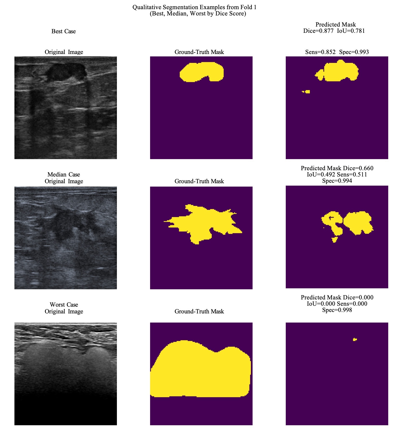
Lastly, we evaluate our image segmentation task whose goal was identifying tumors directly from ultra-sound images. We evaluated four different metrics for this model across our 50 k-folds. The results for the 50 folds are collated in Table 9. From this table we see metrics that reflect the highly imbalanced nature of the segmentation data (i.e. most pixels in a given image are not tumor pixels). These results do not conclusively show our model is able to consistently identify tumors in cases. The Dice score of 0.6 shows some moderate agreement between predictions and ground truth. This is corroborated by an IoU score below roughly 0.46. This score is lower because is a more strict metric penalizing false positives and false negatives more strongly than the Dice score. The specificity and sensitivity indicate that when the model identifies a tumor, it is highly likely to be one, but frequently misses a significant portion of the tumor. To show these results more explicitly, we have plotted a series of figures showing our highest, middling, and lowest performing images. These are shown in Figure 1.

Score	Mean	Min	Max	CI (95%)
Dice	0.59	0.00	0.93	(0.56, 0.62)
IoU	0.46	0.00	0.87	(0.43, 0.49)
Sensitivity	0.58	0.00	1.0	(0.54, 0.61)
Specificity	0.99	0.90	1.0	(0.987, 0.991)

From these figures we can see that while the model is highly successful in some cases, it is woefully inadequate in others. The minimum, maximum spread between metrics succinctly summarizes this issue.

Discussion and Conclusion

The evaluation of our networks shows both the promise and challenges of using deep neural networks in data constrained environments. While the best classification networks worked well, in some cases achieving a .97 ROC AUC score, it is clear from their individual performance that this result is mostly due to the inclusion of the tabular data. The .97 results is, however, a significant achievement indicating a strong ability to distinguish between classes. However as this is a single estimate, this result may not be consistent and should be treated with caution.

The tabular only networks now have only two features including, significantly limiting the predictive power. Although their metrics are not low, the limited input data questions the usefulness of their predictions. Further, the image only networks are unable to accurately distinguish between malignant and benign tumors. Their best performing ROC AUC score of 0.70 is less than that of all of the tabular models. This suggests that the image models are unable to distinguish malignant from benign tumors from the data alone. Lastly, the multi-modal neural networks failed to significantly outperform their constituents. This could be caused due to differences in how the two modes generalize, training gradient blending issues, among other potential issues.

More promisingly, the segmentation network was somewhat effective at identifying tumor regions in breast ultrasound images, as shown by Figure 1. While the Dice score was not extremely high performing (e.g. 0.9), it did reach moderate success at ∼0.6 with a particularly small dataset. This score is slightly lower than other scores achieved both on datasets a factor of ∼2 larger and even a bit smaller than ours (∼0.9 on ∼500 images²⁶, ∼0.87 on 562 images²⁵, and 0.76 on 163 images²⁵.

Ultimately, the performance of our model is limited by the dataset itself. The BrEaST dataset is pretty small and doesn’t have a wide variety of demographic diversity. All the data comes from Poland, which could lead to possible biases in the model’s performance in generalizing to other populations or imaging conditions that are underrepresented in the dataset. Furthermore, the dataset only has high resolution images, which can affect the model’s ability to analyze low resolution images, like those that would come from hospitals in rural areas. Finally, our model was only trained on data where tumor masses were present. Therefore, it would not be good at detecting images where there is no tumor, and would likely draw a mask where there wasn’t a tumor. More data is needed to fully develop the model to be sensitive to normal breast tissue. There are now several available datasets such as those used by²⁵ and²⁶. Future work could evaluate the performance of the models implemented here and in²⁵ and²⁶ on all three datasets individually to compare results and verify how much of the results are dependent on the dataset used. Lastly, while our 50 K-Fold evaluations are better than a single split, still involve the same 252 repeated images and therefore the CIs reflect variability across the split and do not necessarily represent external validity.

Additionally, these findings should be interpreted with important ethical and clinical implementation considerations in mind. Although the models developed here show potential for supporting breast ultrasound assessment, they are not intended to replace radiologist expertise. Rather, they are better understood as adjunctive tools that may assist interpretation and risk assessment within the diagnostic workflow, with clinicians retaining responsibility for evaluating model outputs alongside imaging appearance, patient history, and the broader clinical picture.

Overall, these results should be interpreted as exploratory findings that demonstrate the promise of utilizing deep learning models under constrained data settings. Although the models achieve reasonable performance within the scope of this dataset, these findings should not be interpreted as evidence of current clinical possibility, but rather as an initial investigation into the feasibility and limitations of deep learning approaches in small-data medical settings. Beyond technical refinement, future studies should also consider regulatory readiness, documentation, transparency, and clinical governance requirements as part of model development rather than as downstream concerns.

References

1. H. Sung, J. Ferlay, R. L. Siegel, M. Laversanne, I. Soerjomataram, A. Jemal, F. Bray. Global cancer statistics 2020: GLOBOCAN estimates of incidence and mortality worldwide for 36 cancers in 185 countries. CA: A Cancer Journal for Clinicians, 71(3):209–249, 2021. [↩]
2. W. A. Berg, J. D. Blume, J. B. Cormack, E. B. Mendelson. Operator dependence of physician-performed whole-breast US: lesion detection and characterization. Radiology, 241(2):355–365, 2006. [↩]
3. R. F. Brem, J. Baum, M. C. Lechner, S. S. Kaplan, S. Souders. Improvement in sensitivity of screening mammography with computer-aided detection: A multiinstitutional trial. AJR, Am. J. Roentgenol., 181(3):687–693, 2003. [↩]
4. T. C. Davis, C. L. Arnold, A. Rademaker, S. C. Bailey, D. J. Platt, C. Reynolds, J. Esparza, D. Liu, and M. S. Wolf. Differences in barriers to mammography between rural and urban women. J Womens Health (Larchmt), 21(7):748–755, April 2012. [↩]
5. S. G. Young, M. Ayers, S. F. Malak. Mapping mammography in Arkansas: Locating areas with poor spatial access to breast cancer screening using optimization models and geographic information systems. Journal of Clinical and Translational Science, 4(5):437–442, March 2020. [↩]
6. N. Méndez-Domínguez, M. J. A. Medina, M. B. Gomez, M. E. M. Rojas, E. N. Moreno. Regional inequities in mammography access and utilization in Latin America: Ethnic, rural, and structural barriers identified through a narrative review. Epidemiologia (Basel), 7(1), February 2026. [↩]
7. H. Rehman, I. Ahmad, S. Rashid, M. Mukhtar, A. A. Khan, and H. Khaliq. Comparison of diagnostic accuracy of ultrasound and mammography in detecting breast cancer in radiographically dense breasts. Cureus, 17(9):e92637, September 2025. [↩]
8. J. Wang, S. Zheng, L. Ding, X. Liang, Y. Wang, M. J. W. Greuter, G. H. de Bock, W. Lu. Is ultrasound an accurate alternative for mammography in breast cancer screening in an asian population? a Meta-Analysis. Diagnostics (Basel), 10(11), November 2020. [↩]
9. R. F. Brem, J. Baum, M. C. Lechner, S. S. Kaplan, S. Souders. Improvement in sensitivity of screening mammography with computer-aided detection: A multiinstitutional trial. AJR, Am. J. Roentgenol., 181(3):687–693, 2003. [↩]
10. S. Schrager, V. Ovsepyan, E. Burnside. Breast cancer screening in older women: The importance of shared decision making. Journal of the American Board of Family Medicine, 33(3):473–480, May 2020. [↩]
11. T. M. Kolb, J. Lichy, J. H. Newhouse. Comparison of the performance of screening mammography, physical examination, and breast us and evaluation of factors that influence them: An analysis of 27,825 patient evaluations. Radiology, 225(1):165–175, 2002. PMID: 12355001. [↩]
12. P. A. Carney, D. L. Miglioretti, B. C. Yankaskas, K. Kerlikowske, R. Rosenberg, C. M. Rutter, B. M. Geller, L. A. Abraham, S. H. Taplin, M. Dignan, G. Cutter, R. Ballard-Barbash. Individual and combined effects of age, breast density, and hormone replacement therapy use on the accuracy of screening mammography. Annals of Internal Medicine, 138(3):168–175, 2003. PMID: 12558355. [↩]
13. A. S. Ginsburg, Z. Liddy, P. T. Khazaneh, S. May, F. Pervaiz. A survey of barriers and facilitators to ultrasound use in low- and middle-income countries. Scientific Reports, 13(1):3322, February 2023. [↩]
14. E. Cho, E.-K. Kim, M. K. Song, J. H. Yoon. Application of computer-aided diagnosis on breast ultrasonography: Evaluation of diagnostic performances and agreement of radiologists according to different levels of experience. Journal of Ultrasound in Medicine, 37(1):209–216, 2018. [↩] [↩] [↩]
15. Y. Shen, F. E. Shamout, J. R. Oliver, J. Witowski, K. Kannan, J. Park, N. Wu, C. Huddleston, S. Wolfson, A. Millet, R. Ehrenpreis, D. Awal, C. Tyma, N. Samreen, Y. Gao, C. Chhor, S. Gandhi, C. Lee, S. Kumari-Subaiya, C. Leonard, R. Mohammed, C. Moczulski, J. Altabet, J. Babb, A. Lewin, B. Reig, L. Moy, L. Heacock, K. J. Geras. Artificial intelligence system reduces false-positive findings in the interpretation of breast ultrasound exams. Nature Communications, 12(1):5645, 2021. [↩] [↩] [↩]
16. G. Litjens, T. Kooi, B. E. Bejnordi, A. A. A. Setio, F. Ciompi, M. Ghafoorian, J. A. W. M. van der Laak, B. van Ginneken, C. I. Sánchez. A survey on deep learning in medical image analysis. Medical Image Analysis, 42:60–88, 2017. [↩]
17. J. Kim, H. J. Kim, C. Kim, W. H. Kim. Artificial intelligence in breast ultrasonography. Ultrasonography, 40(2):183–190, 2021. [↩] [↩]
18. Y. Gu, W. Xu, B. Lin, X. An, J. Tian, H. Ran, W. Ren, C. Chang, J. Yuan, C. Kang, Y. Deng, H. Wang, B. Luo, S. Guo, Q. Zhou, E. Xue, W. Zhan, Q. Zhou, J. Li, P. Zhou, M. Chen, Y. Gu, J. Li, L. Cong, L. Zhu, H. Wang, Y. Jiang. Deep learning based on ultrasound images assists breast lesion diagnosis in china: a multicenter diagnostic study. Insights into Imaging, 13(1):124, July 2022. [↩] [↩]
19. K. Dembrower, E. Wa˚hlin, Y. Liu, M. Salim, K. Smith, P. Lindholm, M. Eklund, F. Strand. Effect of artificial intelligence-based triaging of breast cancer screening mammograms on cancer detection and radiologist workload: A retrospective simulation study. The Lancet Digital Health, 2(9):e468–e474, 2020. [↩]
20. S. Pacile`, J. Lopez, P. Chone, T. Bertinotti, J. M. Grouin, P. Fillard. Improving breast cancer detection accuracy of mammography with the concurrent use of an artificial intelligence tool. Radiology: Artificial Intelligence, 2(6):e190208, 2020. [↩]
21. X. Qian, J. Pei, H. Zheng, X. Xie, L. Yan, H. Zhang, C. Han, X. Gao, H. Zhang, W. Zheng, Q. Sun, L. Lu, K. K. Shung. Prospective assessment of breast cancer risk from multimodal multiview ultrasound images via clinically applicable deep learning. Nature Biomedical Engineering, 5(6):522–532, 2021. [↩]
22. M. Xiao, C. Zhao, Q. Zhu, J. Zhang, H. Liu, J. Li, Y. Jiang. An investigation of the classification accuracy of a deep learning framework-based computer-aided diagnosis system in different pathological types of breast lesions. Journal of Thoracic Disease, 11(12):5023, 2019. [↩]
23. S. E. Lee, K. Han, J. H. Youk, J. E. Lee, J.-Y. Hwang, M. Rho, J. Yoon, E.-K. Kim, J. H. Yoon. Differing benefits of artificial intelligence-based computer-aided diagnosis for breast US according to workflow and experience level. Ultrasonography, 41(4):718–727, 2022. [↩]
24. Q. Wei, Y.-J. Yan, G.-G. Wu, X.-R. Ye, F. Jiang, J. Liu, G. Wang, Y. Wang, J. Song, Z.-P. Pan, Jj.-H. Hu, C.-Y. Jin, X. Wang, C. F. Dietrich, X.-W. Cui. The diagnostic performance of ultrasound computer-aided diagnosis system for distinguishing breast masses: A prospective multicenter study. European Radiology, 32(6):4046–4055, 2022. [↩]
25. B. Shareef, M. Xian, A. Vakanski. Stan: Small tumor-aware network for breast ultrasound image segmentation. In 2020 IEEE 17th International Symposium on Biomedical Imaging (ISBI), pages 1–5, 2020. [↩] [↩] [↩] [↩] [↩] [↩]
26. A. Vakanski, M. Xian, P. E. Freer. Attention-Enriched deep learning model for breast tumor segmentation in ultrasound images. Ultrasound in Medicine and Biology, 46(10):2819–2833, July 2020. [↩] [↩] [↩] [↩] [↩]
27. W. Qiu^, E. Hamburg, Y. Zhou, Y. E. Salehani. Lightweight U-Net for breast ultrasound image segmentation. Research Square, 2025. Preprint, PPR:PPR1057279. [↩]
28. A. Pawlowska, A. C´wierz-Pien´kowska, A. Domalik, M. Kowalski, J. Nowak. Curated benchmark dataset for ultrasound based breast lesion analysis. Scientific Data, 11(1):148, January 2024. [↩]
29. D. A. Spak, J. S. Plaxco, L. Santiago, M. J. Dryden, B. E. Dogan. BI-RADS fifth edition: A summary of changes. Diagnostic and Interventional Imaging, 98(3):179–190, 2017. [↩]
30. M. Sandler, A. Howard, M. Zhu, A. Zhmoginov, L.-C. Chen. MobileNetV2: Inverted Residuals and Linear Bottlenecks. In Proceedings of the IEEE/CVF Conference on Computer Vision and Pattern Recognition (CVPR), pages 4510–4520, 2018. [↩]
31. L. Brigato, L. Iocchi. A Close Look at Deep Learning with Small Data. arXiv e-prints, page arXiv:2003.12843, March 2020. [↩] [↩]
32. J. T. Heaton. Introduction to Neural Networks with Java. Heaton Research, Inc., 2005 [↩]
33. D. P. Kingma, J. Ba. Adam: A method for stochastic optimization, 2017. arXiv:1412.6980. [↩]
34. J. T. Heaton. Introduction to Neural Networks with Java. Heaton Research, Inc., 2005 [↩]
35. R. Blaser, P. Fryzlewicz. Random rotation ensembles. Journal of Machine Learning Research, 17(1):126–151, January 2016. [↩]
36. D. Khaledyan, T. J. Marini, T. M. Baran, A. O’Connell, Kevin. Parker. Enhancing breast ultrasound segmentation through fine-tuning and optimization techniques: Sharp attention UNet. PLoS One, 18(12):e0289195, December 2023. [↩] [↩] [↩]
37. M. Latha, P. S. Kumar, R. R. Chandrika, T. R. Mahesh, V. V. Kumar, Suresh. Guluwadi. Revolutionizing breast ultrasound diagnostics with EfficientNet-B7 and explainable AI. BMC Medical Imaging, 24(1):230, September 2024. [↩] [↩] [↩]
38. P. Bruno, M. Macrì, C. Dodaro. A dual-stage deep learning framework for breast ultrasound image segmentation and classification. Journal of Medical Systems, 49(1):162, November 2025. [↩] [↩] [↩]
39. M. Sandler, A. Howard, M. Zhu, A. Zhmoginov, L.-C. Chen. MobileNetV2: Inverted residuals and linear bottlenecks, January 2018. arXiv:1801.04381. [↩] [↩]
40. J. Deng, W. Dong, R. Socher, L.-J. Li, K. Li, L. Fei-Fei. Imagenet: A large-scale hierarchical image database. IEEE Conference on Computer Vision and Pattern Recognition, pages 248–255, 2009. [↩]
41. D. Shen, G. Wu, H. -I. Suk. Deep learning in medical image analysis. Annual Review of Biomedical Engineering, 19:221–248, March 2017. [↩]
42. S. Ioffe, C. Szegedy. Batch Normalization: Accelerating Deep Network Training by Reducing Internal Covariate Shift. arXiv e-prints, page arXiv:1502.03167, February 2015. [↩]
43. K. Simonyan A. Zisserman. Very Deep Convolutional Networks for Large-Scale Image Recognition. arXiv e-prints, page arXiv:1409.1556, September 2014. [↩]
44. N. Srivastava, G. Hinton, A. Krizhevsky, I. Sutskever, R. Salakhutdi-nov. Dropout: A simple way to prevent neural networks from overfitting. Journal of Machine Learning Research, 15(56):1929–1958, 2014. [↩]
45. M. Lin, Q. Chen, S. Yan. Network In Network. arXiv e-prints, page arXiv:1312.4400, December 2013. [↩]
46. A. Saber, T. Emara, S. Elbedwehy, et al. A novel approach for breast cancer detection using a Nesterov accelerated Adam optimizer with an attention mechanism. Scientific Reports, 15:27065, 2025. [↩] [↩]
47. O. Ronneberger, P. Fischer, T. Brox. U-Net: Convolutional networks for biomedical image segmentation, May 2015. arXiv:1505.04597. [↩]
48. W. Qiu, E. Hamburg, Y. Zhou, Y. E. Salehani. Lightweight U-Net for breast ultrasound image segmentation. Research Square, 2025. Preprint, PPR:PPR1057279. [↩]
49. S. Jadon. A survey of loss functions for semantic segmentation. arXiv e-prints, page arXiv:2006.14822, June 2020. [↩]