Examining the Predictive Value of Rainfall Variability beyond Cumulative Rainfall for Harmful Algal Bloom Modeling Using Machine Learning

Abstract

Harmful algal blooms (HABs) can negatively affect aquatic ecosystems by creating hypoxic conditions and releasing toxins into the water. Rainfall drives HAB growth by allowing runoff containing nutrients and fertilizers, such as nitrogen and phosphorus, to enter waterways. Therefore, many prediction models rely on total rainfall but overlook the impact of rainfall variability on algae growth. This study tested whether rainfall variability improves models’ predictions of elevated chlorophyll-a levels compared to cumulative rainfall in western Lake Erie from 2013 to 2023. Three random forest models were trained using chlorophyll-a samples and daily precipitation, each with a different set of features: one with 7 and 30-day rainfall totals only, one with 7 and 30-day standard deviations, coefficients of variation, and wet days (precipitation greater than 0.01 mm), and one with all of these features combined. Each model was trained using samples from 2013-2020 and tested on samples from 2021-2023, with each model predicting whether a sample contains elevated chlorophyll-a levels. The totals-only model performed the best on ranking metrics such as ROC-AUC and PR-AUC, while the variability-only and combined models performed slightly better than totals-only on threshold-based metrics such as balanced accuracy and F1. These results indicate that rainfall variability may have modest predictive value beyond total rainfall in predicting above-median chlorophyll-a levels, although the absence of nutrient and temperature data, along with spatial constraints, somewhat limits the generalizability of the results.

Keywords: HABs, Lake Erie, algae, rainfall, machine learning, rainfall variability

Introduction

Harmful algal blooms (HABs) threaten many freshwater ecosystems, as they deplete oxygen in water and release toxins such as microcystins into the environment¹. Rainfall contributes to the growth of algae by driving runoff full of nutrients into bodies of water. A growing number of studies have started to investigate the relationships between algae growth, total rainfall, and rainfall distribution. Rainfall variability can alter runoff composition independently of total rainfall², extreme rainfall can disproportionately increase the amount of nutrients such as phosphorus entering waterways³, short and intense storms can result in waves of nutrients which totals-based models miss⁴, and analyses show a link between heavy, shifting precipitation and changes in water quality⁵. Although rainfall can increase the amount of nutrients in waterways⁶, it can also dilute and flush them out as well⁷. As a result, algae prediction models relying only on total rainfall face the risk of missing runoff processes driven by varied-rainfall events such as clustered storms⁶.  Even though variability is recognized as a growth factor, its use in predictive machine learning models is still relatively low.

Tree-based models such as random forest and XGBoost have been used in multiple studies to predict chlorophyll-a levels, due to their ability to find non-linear relationships^8,9. Studies of western Lake Erie have mainly identified nutrients and physicochemical variables as the central drivers of algae growth, with rainfall contributing very little^10,11. However, these studies represent antecedent rainfall (if even used at all) as a cumulative total in their models, and rarely test if rainfall variability actually has predictive value beyond just total rainfall.

This study seeks to fill that gap by answering the question of whether the use of rainfall variability metrics has an effect on improving predictions of elevated chlorophyll-a levels compared to the standalone metric of total rainfall. To answer this question, three random forest models containing different sets of features were trained and tested on precipitation and chlorophyll-a datasets so as to compare and evaluate each metric’s contribution. Random forest models were chosen in particular due to their ability to model non-linear relationships between rainfall variability and chlorophyll-a. The models aimed to predict elevated levels of chlorophyll-a, with model performances being evaluated through standard machine learning benchmarks such as balanced accuracy, ROC-AUC, and F1. In order to maintain the scope of the study and limit outside influences on the results of the experiment, the models were trained and tested exclusively with rainfall data, with other algal growth factors being omitted.

Methods

This study concentrates specifically on Lake Erie from 2013 to 2023, as it has historically been affected by HABs and also because there is an abundance of both climate and chlorophyll-a datasets available¹². The purpose of this study is to compare three random forest models using various feature sets (total rainfall, rainfall variability, and both combined, respectively; each feature set also includes month) to predict above-median chlorophyll-a concentrations.

The precipitation dataset used contains daily precipitation totals from NOAA weather station USW00094830 (Toledo Express Airport, OH; 41.59°N, 83.81°W; accessed 4/11/2026) located on the western end of the lake. The second dataset used was obtained from the NOAA’s National Centers for Environmental Information (NCEI) website (dataset name: Physical, chemical, and biological water quality monitoring data to support detection of Harmful Algal Blooms (HABs) in western Lake Erie, collected by the Great Lakes Environmental Research Laboratory and the Cooperative Institute for Great Lakes Research since 2012; accessed 4/12/2026), out of which chlorophyll-a samples that span across western Lake Erie were obtained¹³.

Toledo Express precipitation data was used to calculate antecedent rainfall features for all of the chlorophyll-a samples, regardless of sample location. Chlorophyll-a samples were located 32.7-214.9 km away from the Toledo Express weather station (median of 78.8 km) and 1.8-184.2 km away (median of 48.3 km) from the Maumee River mouth reference point used in this study (41.70°N, 83.45°W). No additional bounding box/watershed feature was applied beyond the western Lake Erie extent of the chlorophyll coordinates. Although both datasets geographically correspond to western Lake Erie, the vastness of the lake and the spatial distribution of climate and chlorophyll samples represent a limitation that predictions are unlikely to apply across the entire lake. As such, associations represented in this study merely represent single gauge relationships and should not be interpreted as spatially resolved rainfall patterns.

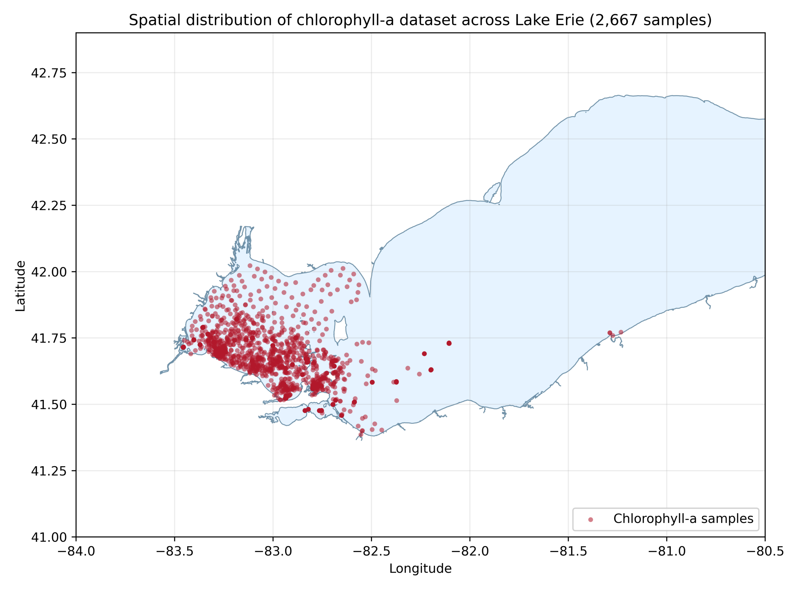
To process the datasets, chlorophyll-a and precipitation sampling records were limited to 2013-2023, converted to standard ISO dates, and had numeric formatting applied to chlorophyll-a and coordinate points. Rows which did not have either a valid sample date or chlorophyll-a values were then removed. Duplicate records with shared calendar dates were saved as separate entries rather than being combined into a single sample. 2,667 samples were left after cleaning and processing the datasets, each with corresponding chlorophyll-a and precipitation values.

The training to test split of data used a temporal split instead of a predetermined percentage split. The training dataset consists of all values from 2013-2020 (2,079 samples), while the test dataset consists of the remaining data samples from 2021-2023 (588 samples). A temporal split was used because it tests forward generalization on the 2021-2023 test set after training on the 2013-2020 data. A random percentage-based split could place samples from the same seasons or years in both the training and testing sets, which would spread year-specific conditions across both datasets and lead to inflated model performance.

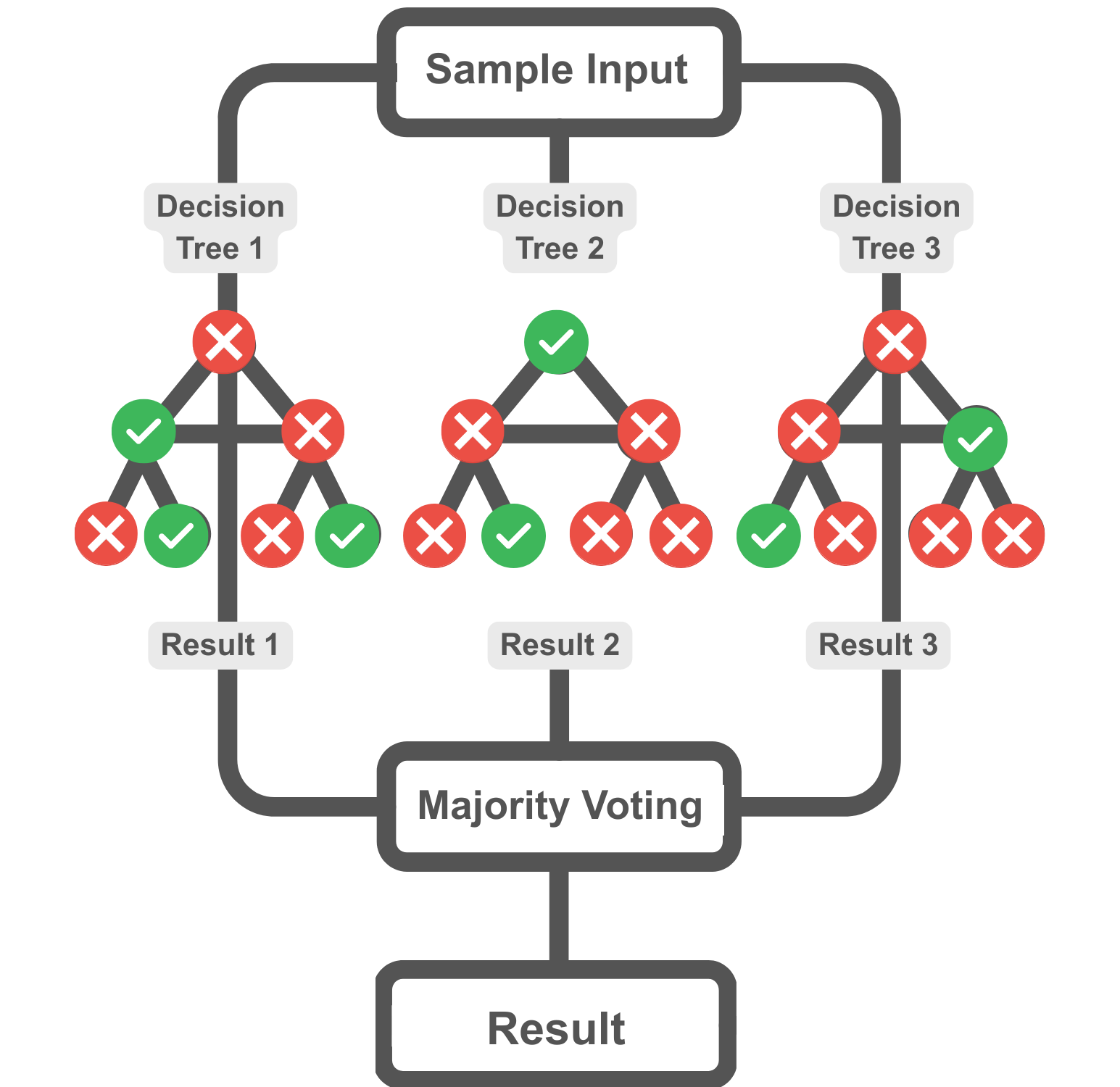
A random forest model was chosen to make predictions due to its ability to process data in nonlinear relationships. This type of model also allows for hyperparameters to stay constant across all the models in order to ensure that differences in results are due to feature sets only. Boosting methods such as Gradient Boosting and XGBoost were considered but not used because they require additional tuning (learning rate, subsampling, and regularization) that could add another source of variation and potentially complicate the interpretation of modest and metric-dependent results^14,15,16. Antecedent rainfall features were calculated over two rolling windows of lengths 7 and 30 days, respectively. A 7-day window was chosen to target short-term runoff¹⁷, while a 30-day window was chosen to capture longer rainfall conditions consistent with bloom season moisture accumulation¹⁸. Non-overlapping windows were not used because they would add more features and push the study to become more of a window selection analysis rather than a controlled model comparison.

Rainfall features for each sample were calculated only with daily precipitation leading up to/during the 7 or 30 day windows (including the sample date), with missing precipitation days counted as zero rainfall (0 mm). This process guarantees that rainfall after the current window being analyzed by the model cannot affect the predictions. Daily precipitation was recorded as total rainfall within the day, without taking into account when exactly during the day rainfall occurred. This means that rainfall could have occurred after the sample was taken, which would lead to some samples including post-sampling rainfall. This potential contamination was limited to at most one day within each 7/30-day window, and notably is also common within standard runoff modeling.

Within every single window, 4 separate features were calculated: a sum of total rainfall, standard deviation of daily rainfall, coefficient of variation (calculated by standard deviation / (absolute mean + 1 × 10⁻⁶) to avoid division by 0), and a ‘wet-day’ count (number of days with precipitation greater than 0.01 mm). Feature distributions in the training set were checked for extreme CV values (Figure 10), and CV was not winsorized. Because random forest models split on thresholds and not exact values, monotonic rescaling of CV would not affect tree structure. All 4 of the features mentioned above were calculated using the same daily rainfall data, and, as a result, are correlated. An additional ‘month’ feature was added as well in order to have a seasonality control. Code used to generate features is available in supplementary materials.

Chlorophyll-a levels were designated as ‘elevated’ if they were greater than or equal to 9.51 µg L⁻¹ (median chlorophyll-a level in 2013-2020 training data), and model predictions were evaluated at a probability threshold of 0.5. A median split was chosen because it can help answer the main research question of how well the models identify higher/lower than usual chlorophyll-a levels by establishing a dataset-specific and objective split. Additionally, a median yields two approximately balanced training classes consisting of around 50% elevated/non-elevated samples each, which helps with stabilizing random forest model training and evaluation¹⁹. Ecological/regulatory cutoffs were not used because they may not match this dataset’s unique distribution of samples and mainly target management/identifying bloom events instead of above-median chlorophyll-a levels.

The random forest models were built with Python using the libraries pandas 3.0.0, NumPy 2.4.1, and scikit-learn 1.8.0. Each model consists of 150 decision trees that split on a random subset of the calculated features at every node with a maximum depth of 12, minimum leaf size of 12, balanced class weight, random_state = 42, criterion = gini, max_features = sqrt, and scikit-learn defaults for the remaining hyperparameters. The three models were each equipped with a varied set of features: one with 7 and 30-day rainfall totals only, one with 7 and 30-day standard deviations, coefficients of variation, and wet days, and one with all of these features combined. As mentioned before, the month feature is also present in all 3 of the models to account for seasonality. In order to quantify the performance of seasonality, a month-only baseline random forest model was trained as well (Table 3).

Model performance on the 2021-2023 test set was evaluated by balanced accuracy, ROC-AUC, F1, PR-AUC, sensitivity, specificity, precision, and negative predictive value (NPV) at a probability threshold of 0.5 (Table 1). The comparisons among the rainfall feature sets in Tables 1 and 2 should be interpreted as conditional on month for all three models. Pairwise differences in model performances were assessed with 2000 paired bootstrap samples to achieve 95% confidence intervals for each metric (Table 2). Because the results vary by metric, the conclusions are reported as metric-dependent instead of identifying a single ‘best’ model. ROC and precision-recall curves (Figure 4), confusion matrices at the 0.5 threshold (Figure 5), and threshold sensitivity analyses at probabilities of 0.3, 0.4, 0.5, and 0.6 (Figure 6) were created to display the various tradeoffs between models.

Features with the highest importance were determined by analyzing mean decrease in Gini impurity^20,21. Both Gini importance from the training data and permutation importance from the testing data (balanced accuracy with 30 shuffles and fixed seed of 42) are reported for the combined model (Figures 8 and 9). However, because standard Gini/permutation importance is unreliable with collinear predictors, grouped ablation was used as the primary correlation-robust importance. Grouped ablation was conducted by retraining a random forest model after a single feature set- rainfall totals (amount), wet-day counts (frequency), or standard deviation + coefficient of variation (dispersion)- was removed while retaining month (Table 3). The relationships among inputs and rainfall features by above-median vs. below-median chlorophyll are shown in Figure 7 (Pearson feature correlation matrix) and Figure 10 (rainfall feature distributions by chlorophyll class).

As a sensitivity check under the single-gauge spatial limitation of the precipitation data, the test set data was reevaluated by distance tertiles to see whether model performances and totals vs. variability patterns would hold across sample distances. The training set data was used to create three tertiles (‘near’, ‘mid’, and ‘far’) which were applied unchanged to the test set separately for distance to both Toledo Express and the Maumee River mouth. The models were not retrained for each tertile, meaning that the same rainfall features were applied to all samples within each tertile. The results of distance tertile testing are summarized in Table 4.

Results

In testing, each model predicts whether chlorophyll-a values will cross the threshold of 9.51 µg L⁻¹, with 0 representing a prediction of ‘no’ and 1 representing a prediction of ‘yes’. The results of the models’ performance on the 2021-2023 test dataset are summarized in Table 1, with Figure 4 displaying ROC-AUC and precision-recall curves.

Model	Balanced Accuracy	ROC-AUC	PR- AUC	F1 (elevated)	Sensitivity	Specificity	Precision	NPV
Totals-only	0.680	0.763	0.657	0.631	0.800	0.560	0.521	0.824
Variability- only	0.711	0.740	0.608	0.640	0.646	0.777	0.634	0.786
Combined (totals + variability)	0.714	0.745	0.622	0.644	0.655	0.775	0.634	0.790

The balanced accuracy measure tracks the performance of the model in identifying both elevated and non-elevated levels of chlorophyll and weighs each class equally. ROC-AUC values are a measure of how accurately the model’s predicted probabilities rank elevated and non-elevated samples, and F1 values balance the accuracy of the model in catching the elevated chlorophyll-a levels and avoiding overpredictions. PR-AUC represents the trade-off between model precision and recall, and provides a measure to assess how well the model identifies elevated chlorophyll-a levels when the classes are imbalanced. Sensitivity refers to how well the model correctly identifies elevated levels of chlorophyll, while specificity refers to how well the model correctly identifies non-elevated levels of chlorophyll. Precision values were calculated by how many elevated cases were predicted correctly, and NPV scores reflect how many non-elevated cases the model predicted correctly.

Each of these values offers insight into how the models performed and the overall impact of each feature set on model performance. Balanced accuracy scores reflect the fact that adding variability features can potentially help the model recognize elevated and non-elevated levels of chlorophyll, with the variability-only and combined models each outperforming the totals-only model by a borderline margin. Modest F1 gains suggest the importance of variability features, with the combined and variability-only models once again outperforming the totals-only model. That said, the month-only baseline achieved the highest overall balanced accuracy and F1 scores (Table 3). The ROC-AUC values stand out because the totals-only model outperforms both other models in ranking elevated and non-elevated sample predictions. PR-AUC values reflect a similar outcome, as the totals-only model once again achieved the highest value and surpassed both the variability-only and the combined models. These results reveal that model performance is mainly metric-dependent, as each model performed better on certain metrics and worse on others.

The remaining four metrics- sensitivity, specificity, precision, and NPV- all highlight various tradeoffs between models. For example, the totals-only model has the highest sensitivity (0.800), but also has the lowest specificity (0.560) and precision (0.521), revealing that this model is more aggressive in identifying elevated chlorophyll-a levels but with the tradeoff of creating more false positives as well. The variability-only and combined models differ compared to the totals-only model, as they both have lower sensitivities and higher specificity and precision values. These findings suggest that overall, the variability-only and combined models are better at avoiding false positives compared to the totals-only model, but at the cost of a lower sensitivity. Finally, NPV values across all models are relatively high, which indicates that non-elevated predictions are generally accurate.

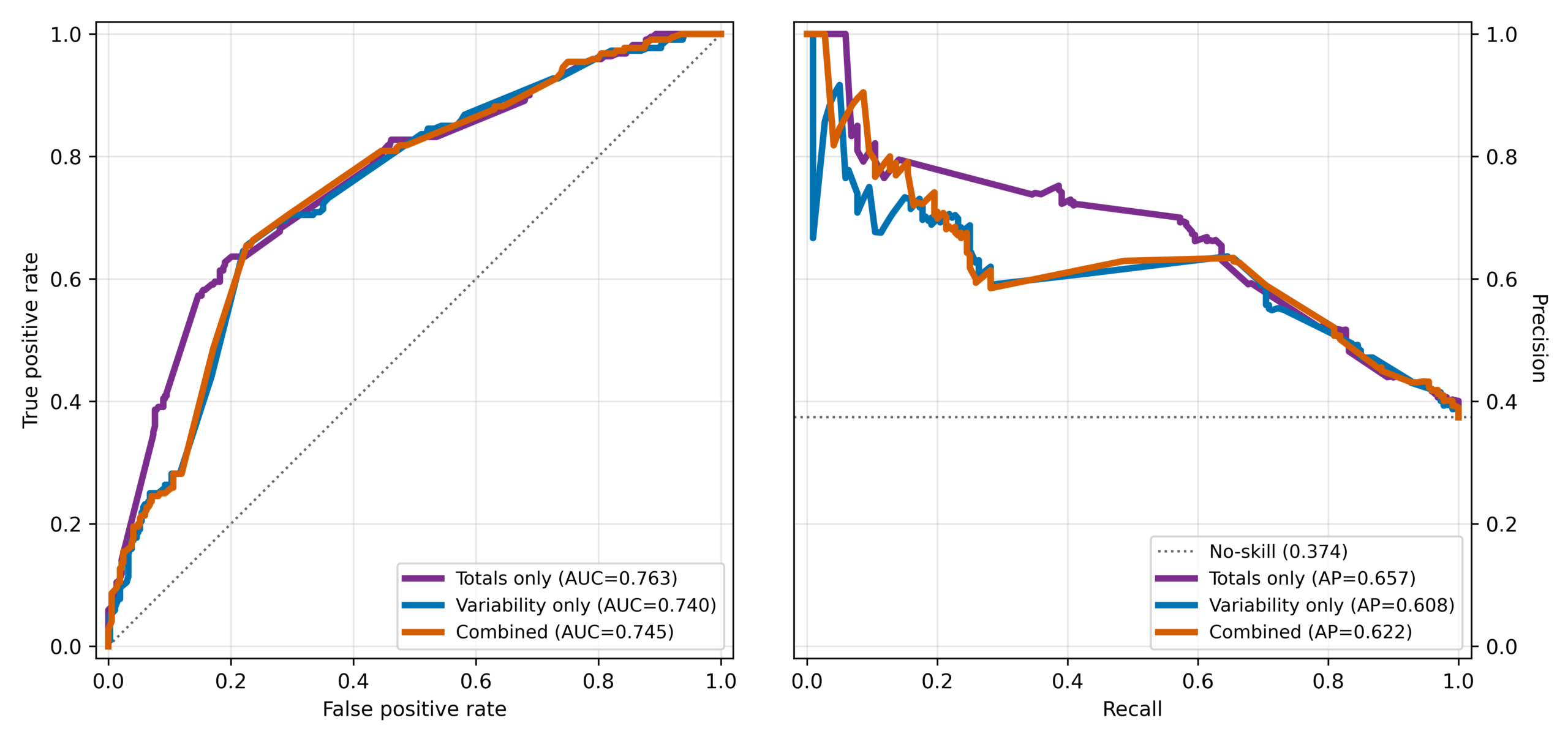
The ROC curves illustrated by Figure 4 display how each model performs across different classification thresholds. The totals-only model outperforms both other models by a modest margin, suggesting that total rainfall provides the strongest separation even though predictions at the 0.5 threshold are less balanced. Similar to the ROC-AUC results, the totals-only model once again achieved the best PR-AUC among the models. These findings indicate that the totals-only model performs best at creating probability-based rankings, while the variability-only and combined models perform slightly better in scenarios with threshold-based metrics.

In order to determine whether differences in metrics are meaningful or are due to random variation, pairwise comparisons were conducted using bootstrap confidence intervals, the results of which are displayed in Table 2.

Metric	Totals vs Variability Δ (95% CI)	Totals vs Combined Δ (95% CI)	Variability vs Combined Δ (95% CI)
Balanced Accuracy	0.0314 (-0.001, 0.0619)	0.0346 (0.0022, 0.0668)	0.0032 (-0.0028, 0.0107)
ROC-AUC	-0.0227 (-0.0456, 0.0004)	-0.0181 (-0.0384, 0.0008)	0.0046 (-0.0099, 0.0187)
F1	0.0088 (-0.0307, 0.0471)	0.0135 (-0.0267, 0.0531)	0.0047 (-0.0029, 0.0149)
PR-AUC	-0.0489 (-0.0919, -0.0072)	-0.0347 (-0.0695, -0.0008)	0.0141 (-0.0080, 0.0366)

Across pairwise differences, balanced accuracy and PR-AUC are the only metrics with statistically significant differences. The balanced accuracy improvement of the combined model over the totals-only model is statistically significant, meaning that the performance gap between these two models is in all likelihood real and not attributable to chance, while the balanced accuracy difference between totals-only and variability-only is borderline and not clearly significant. To contrast, PR-AUC values indicate a statistically significant decrease in performance associated with the variability-only and combined models compared to the totals-only model, suggesting a trade-off between an improvement in classification performance and a decreased precision-recall performance. For the ROC-AUC and F1 metrics, there are no statistically significant differences, which suggests that the differences are small and do not have a meaningful effect on the results. Similarly, there are no statistically significant differences in any metrics between the variability-only and combined models.

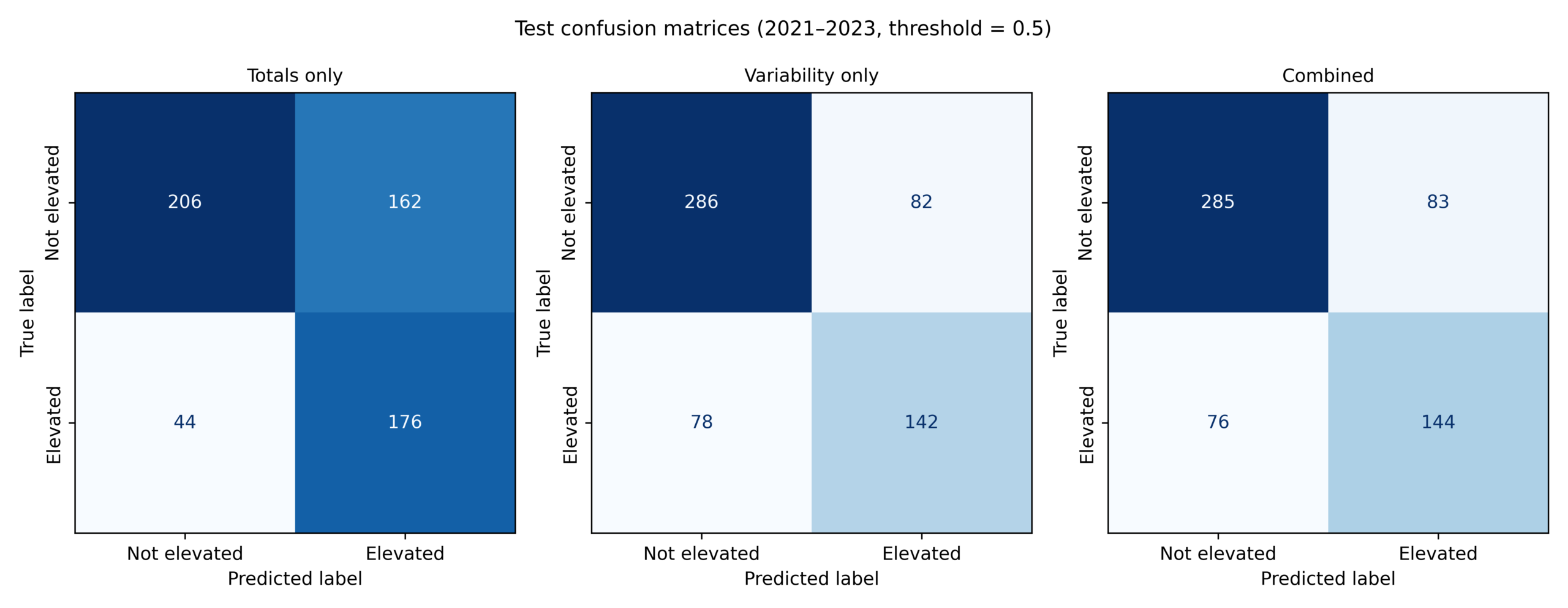
Looking at the models’ confusion matrices of the test dataset, the totals-only model made the greatest number of incorrect predictions (206 total incorrect predictions), but was also able to correctly predict 176 samples as elevated, which is the highest among all of the models. The variability-only and combined models’ predictions were almost exactly the same, with a slight amount of variation. Each cell between the two models differed by only one or two samples, which aligns with the results of Table 2, in which every bootstrap interval between the variability-only and combined models included zero. The clear presence of incorrect predictions highlights the need for additional features, such as nutrient loading and water temperature, to be added for the model to achieve greater accuracy and more consistent results.

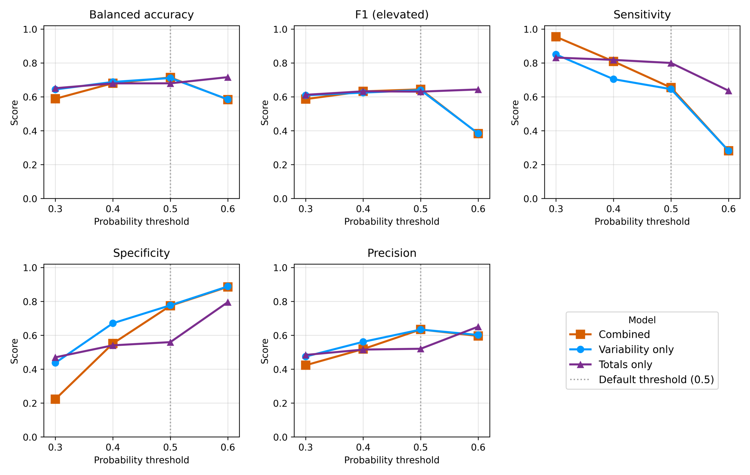
To understand the effects different thresholds would have upon the results, a threshold sensitivity analysis from probability cutoffs of 0.3-0.6 was conducted (Figure 6). The analysis reveals that model performance depends on the threshold being used to classify predictions. At the default 0.5 threshold, the variability-only and combined models either outperformed or achieved similar performance to the totals-only model on all metrics except sensitivity. At the lowest threshold of 0.3, the combined model earned the highest sensitivity but also the lowest specificity, meaning that lower thresholds made the model predict more samples as elevated. Moving from 0.5 to the highest threshold of 0.6, the variability-only and combined models’ performances started to decrease in every metric except specificity, in which it continued to increase. On the contrary, the totals-only model began to outperform both other models in every metric except specificity at the 0.6 threshold, highlighting the sensitivity-specificity tradeoff between the models’ performances. The results of this analysis overall show that across all of the thresholds, the variability-only and combined models’ performances remained similar to each other, and that model performance depends on both the probability threshold and the metric chosen.

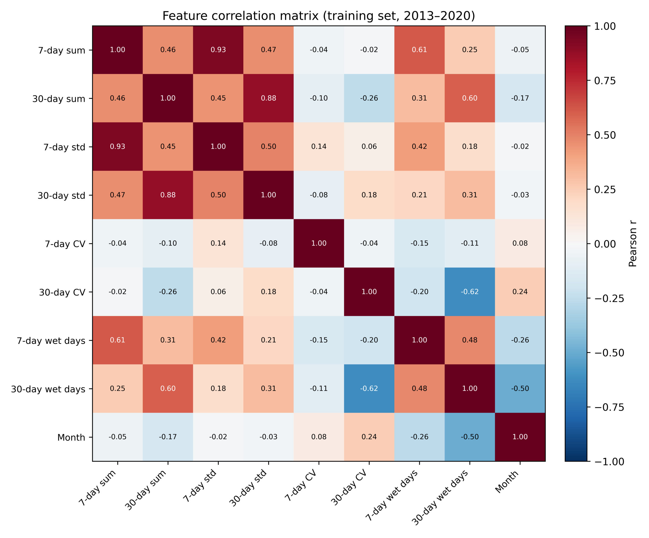
Figure 7 reflects that rainfall amount, frequency, and dispersion metrics were all strongly correlated in the training dataset because they were all calculated from the same daily precipitation series within each window. The strongest associations were between total rainfall and standard deviations, especially in the cases of 7-day std vs. 7-day sum (r = 0.93) and 30-day std vs. 30-day sum (r = 0.88). Rainfall sums and wet days were also correlated, as demonstrated by 7-day sum vs. 7-day wet days (r = 0.61) and 30-day sum vs. 30-day wet days (r = 0.60), while the strongest negative correlation was between 30-day CV vs. 30-day wet days (r = -0.62). These results highlight that short-term, highly variable rainfall can occur with fewer wet days over longer rainfall periods. Although near-zero mean windows can result in larger CV ratios, the training set data was inspected and not winsorized, showing a limited 7-day CV range of 0 to 2.65. Overall, the correlations represented in Figure 7 suggest that individual rainfall features cannot be treated as independent predictors, and that differences in prior rainfall conditions are driven by combined patterns instead of singular metrics.

Model	Balanced Accuracy	ROC-AUC	F1	PR-AUC
Full combined	0.714	0.745	0.644	0.622
Drop amount	0.711	0.740	0.640	0.608
Drop frequency	0.711	0.735	0.640	0.616
Drop dispersion	0.679	0.764	0.629	0.648
Amount-only	0.680	0.763	0.631	0.657
Frequency-only	0.705	0.756	0.639	0.615
Dispersion-only	0.580	0.729	0.379	0.605
Month-only (Baseline)	0.721	0.740	0.650	0.585

Grouped ablation performed on the test set revealed how much each feature group in the combined model actually contributed to the results. The month-only baseline model achieved balanced accuracy and F1 scores higher than any of the rainfall-inclusive models. Compared to the full combined model, dropping rainfall totals (amount) or frequency led to small decreases in model performance across all metrics. Removing the dispersion group caused a larger drop in performance across balanced accuracy and F1 while also resulting in an increase in ROC-AUC and PR-AUC, highlighting some of the tradeoffs between metrics. Across the single-group models, the amount-only and frequency-only models performed considerably better compared to the dispersion-only model across both balanced accuracy and F1, and slightly better across ROC-AUC and PR-AUC. Notably, the amount-only model also performed exactly like the totals-only model (Table 1), with identical results across all of the metrics. The performance of the dispersion-only model indicates that although variability metrics alone are not very strong predictors, they contribute meaningfully to threshold metrics. Overall, these results reveal that amount and frequency are the main feature sets adding ranking metric value while no model improved on the month-only model’s performance in threshold metrics.

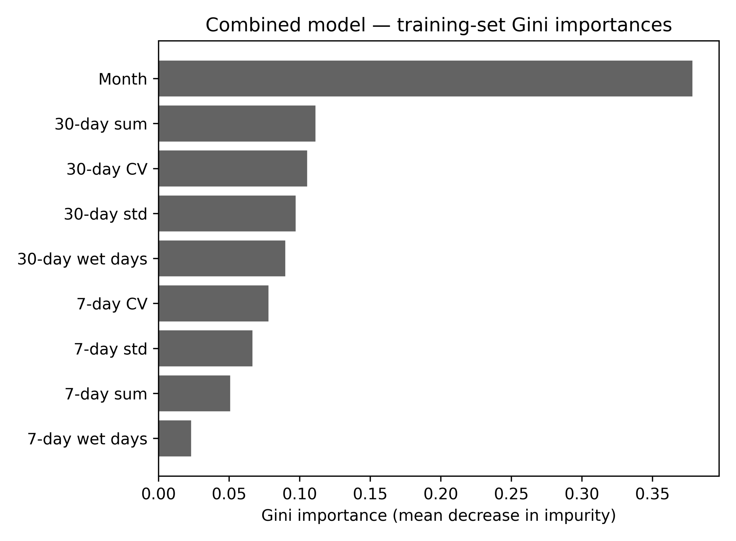
Looking at the feature importance chart, month has the highest importance (0.38) by a considerable margin of 0.27. The next highest importances are 30-day rainfall totals (0.11), 30-day CV (0.105), 30-day std (0.10), and 30-day wet days (0.09). 7-day features follow behind the 30-day features, revealing that the model relies more on long-term intervals for predictions.

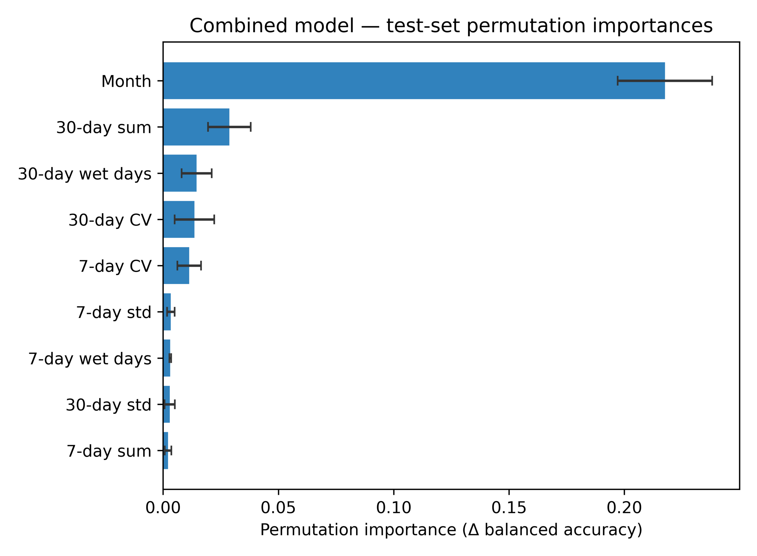
Similar to the Gini importances, the feature with the highest permutation importance is month. Shuffling month caused balanced accuracy to reduce by 0.22 (± 0.02 across 30 repeats). Rainfall features were quite low, as in the case of 30-day sum (0.029), 30-day wet days (0.015), 30-day CV (0.014), and 7-day CV (0.011). The remaining features (7-day std, 7-day wet days, 30-day std, and 7-day sum) all had near-zero effects, suggesting their low predictive value compared to month and the higher importance features. Because month was in all three models, the results in Table 1 should be interpreted as comparing rainfall feature sets after accounting for seasonality. Higher Gini importances for standard deviation also did not match with lower std permutation importances, likely due to standard deviation overlapping strongly with sum (Figure 7).

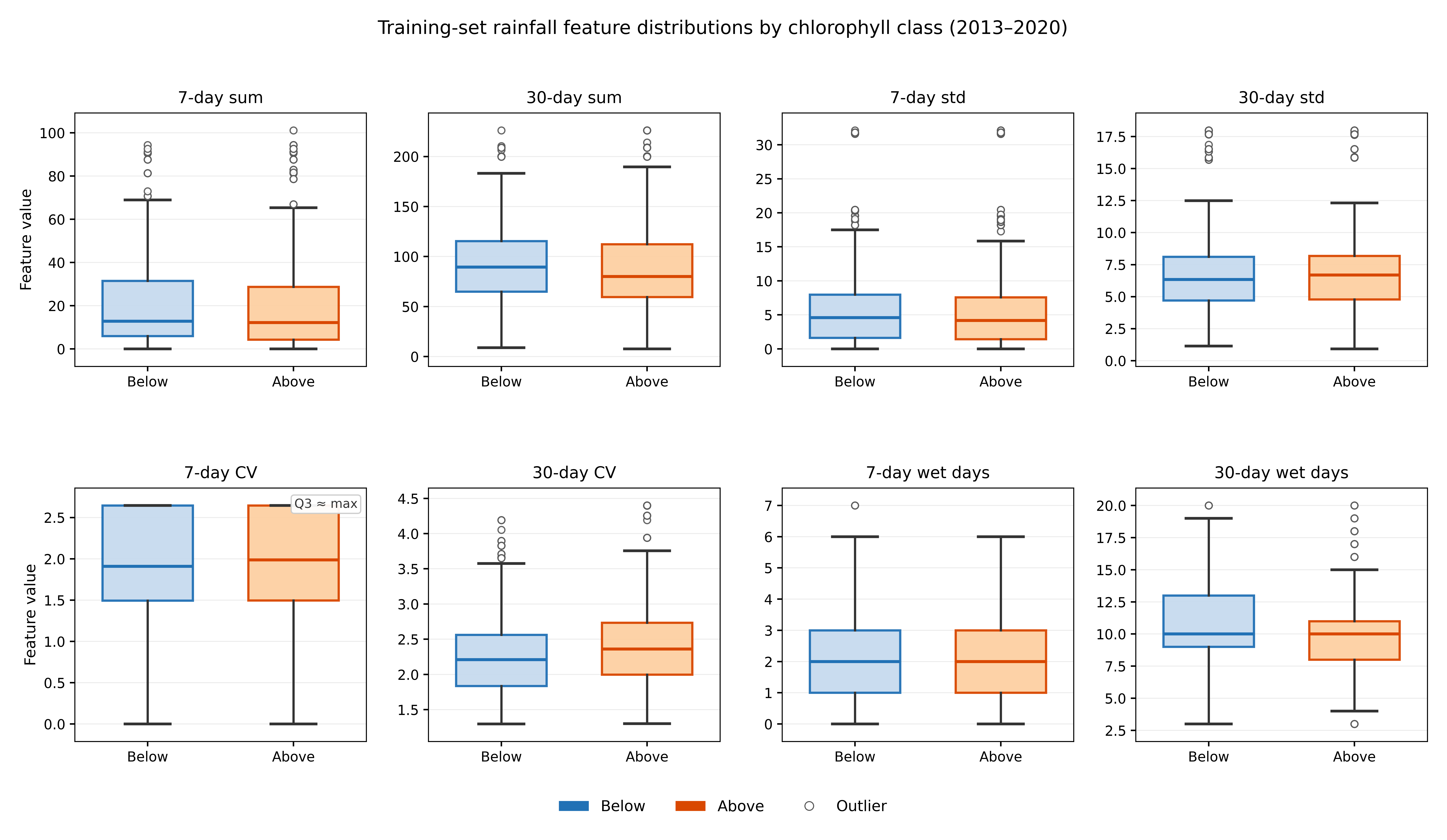
Figure 10 further displays variations between feature differences, more specifically between above-median and below-median chlorophyll classes in the training set. Differences were most visible for 30-day metrics, with above-median samples having slightly higher 30-day CVs (2.36 vs. 2.21) and 30-day standard deviations (6.68 vs. 6.34), and below-median samples having higher 30-day sums (89.4 vs. 80.0). 7-day metrics and wet day counts were more similar between classes, evidenced by both 7-day and 30-day wet days having the same median for both above-median and below-median classes (2 and 10 days, respectively). The substantial overlap between all of the features suggests that there is no singular metric that separates the classes clearly. This supports both the correlation results from Figure 7 as well as the interpretation that rainfall features should be treated as complementary predictors rather than individual regressors.

Reference	Tertile	Distance (km)	n	Totals	Variability	Combined
Toledo Express	Near	32.7-70.9	235	0.639	0.692	0.701
	Mid	70.9-82.2	223	0.734	0.750	0.747
	Far	82.2-214.9	114	0.711	0.830	0.830
Maumee River mouth	Near	1.8-41.6	237	0.641	0.691	0.700
	Mid	41.6-52.3	245	0.714	0.745	0.742
	Far	52.3-184.2	92	0.757	0.863	0.863

Examining the results displayed in Table 4, the ‘near’ tertile’s balanced accuracies between both references are almost identical because 234 of the 235 Toledo Express ‘near’ samples are also shared with the Maumee River mouth ‘near’ samples. Across both references, the models performed the worst in the ‘near’ tertile, and in the ‘mid’ and ‘far’ tertiles, the variability-only and combined models performed as well as or better than the totals-only model. Balanced accuracy being higher for ‘far’ samples despite having smaller sample sizes (n = 114 and 92) does not reflect a stronger local rainfall signal, and is more likely a result of small sample sizes, differences in class balances, and a greater influence of seasonality on offshore samples. The data used in the table is a smaller subset of the full testing data, used the same single-gauge rainfall data, and was not retrained separately, meaning that the results should be considered exploratory. Although this test does not address the actual single gauge limitation, it suggests that the overall patterns between total rainfall and rainfall variability are not driven only by samples nearest to the shore.

Discussion

The results revealed that the variability-only model slightly outperformed the totals-only model in balanced accuracy and F1 scores, and the combined model did so as well, but by a greater margin. The totals-only model did better than both of the other models in terms of ROC-AUC and PR-AUC values, pointing to its strength in ranking elevated and non-elevated samples. The variability-only and combined models achieved higher specificity scores (~0.77) at the cost of a lower sensitivity (~0.65) compared to the totals-only model (0.80 sensitivity and 0.56 specificity). Threshold sensitivity analysis revealed that model rankings are not the same across different decision thresholds, indicating that results are mainly metric dependent. Since the month-only model displayed the highest performance on threshold metrics, it suggests that much of the threshold accuracy depends on month, and that rainfall features mainly help with performing ranking metrics.

Across paired bootstrap comparisons, the combined model displayed a slight statistically significant improvement in balanced accuracy over that of the totals-only model. Other than this slight improvement, however, the combined model did not meaningfully outperform the variability-only and totals-only models across any of the metrics. These findings suggest that rainfall variability provides limited information beyond total rainfall in predicting chlorophyll-a levels, but does not consistently outperform cumulative rainfall.

Feature importance charts (Figures 8 and 9) offer further insight on what the models relied on to make predictions^20,21. Month was ranked the highest feature for both Gini and permutation importance, which is expected due to seasonal bloom timing having a large impact on algae growth and chlorophyll-a levels. 30-day rainfall metrics were the next most important features, adding a substantial amount of predictive value beyond month. As mentioned before and displayed in Figure 7, all rainfall features are correlated because they are calculated from the same data and time series. Grouped ablation (Table 3) revealed that amount (rainfall totals) and frequency (number of wet days) had the most predictive value within the combined model, with dispersion (variability features) having a weak standalone performance but adding a notable gain to threshold metrics. 

There are several main limitations that should be taken into consideration when interpreting the results of this study. First, precipitation comes from just a single gauge, meaning that spatial variability across Lake Erie and the broader Maumee watershed (Lake Erie’s western basin) is unable to be captured or represented in this study. A distance-stratified re-evaluation of the test set (Table 4) did show that totals vs. variability patterns were not driven solely by samples closest to the shore, but this analysis is exploratory and does not fully address the limitation. Second, while chlorophyll samples are sparse and seasonal, rainfall data is available daily. This results in the models being trained and tested only on days where both chlorophyll and rainfall data are available, with the gaps between samples being omitted from the data used.

The third limitation is that the median threshold of 9.51 µg L⁻¹ is just a statistical split used for the purpose of this study, and does not have any ecological significance. This means that above-median chlorophyll-a samples do not necessarily represent operational bloom events, as it does not constitute a regulatory or management threshold. Fourth, the models were neither trained nor tested on common drivers of algae growth, such as nitrogen and phosphorus levels, temperature data, and wind^22,23, instead being trained exclusively with precipitation and chlorophyll-a data. Therefore, variability features may partly represent these missing drivers²⁴, meaning that rainfall variability cannot be read as a fully independent ecological predictor. The fifth and final limitation is that antecedent rainfall was calculated only within 7-day and 30-day windows, with other lag patterns not being evaluated and requiring future work.

There are many ways that future work can expand on this study before expanding to operational usage, such as: testing the impact of watershed-scale gridded and radar-derived precipitation, precipitation data from multiple stations, and basin-averaged rainfall on totals vs. variability; using non-overlapping/ecologically significant windows to calculate rainfall features; and expanding the models to include additional algal driver data such as Maumee River discharge, nutrient samples, water temperature, remotely sensed bloom extent²⁵, and wind, as well as baseline models to separate rainfall variability features from algal drivers²⁶. Using longer testing timeframes and gaining validation outside of Lake Erie would also help clarify if model gains generalize beyond this study’s observation period and location.

This study examined the effect of rainfall variability metrics on predicting chlorophyll-a in western Lake Erie by comparing three models with distinct sets of features. The results are metric-dependent and modest, with no model completely outperforming the other two. The totals-only model performed the best on ranking metrics such as ROC-AUC and PR-AUC, while the variability-only and combined models performed slightly better than the totals-only model on threshold-based metrics such as balanced accuracy and F1. Overall, it can be concluded that rainfall variability may add slight predictive value in more complete models with spatially resolved precipitation and algal drivers accounted for, but is not sufficient enough for standalone bloom forecasting.

Gains in model accuracy are crucial because they can aid early detection efforts and help support responses to bloom events. In 2014, Lake Erie was affected by a severe algae bloom which released toxic microcystins into the Toledo water supply, leading to over 400,000 residents being left without water²⁷. This tragedy led to the creation of the NOAA HAB forecast system and continues to serve as an important reminder of the role algae monitoring systems play in keeping citizens safe and prepared. By continually improving prediction models and understanding environmental systems’ impact on algae growth, future tragedies can be dealt with more efficiently or even avoided entirely.

Acknowledgements

I would like to acknowledge the NOAA for providing both datasets used to conduct this study. I would also like to thank my mentor, Gary Mavko, for supporting me throughout the research process.

Supplementary Information

References

1. H. W. Paerl. Nuisance phytoplankton blooms in coastal, estuarine, and inland waters. Limnology and Oceanography. Vol. 33, pg. 823–843, 1988, https://doi.org/10.4319/lo.1988.33.4part2.0823. [↩]
2. W. Zhou, Z. Zhu, Y. Xie, Y. Cai. Impacts of rainfall spatial and temporal variabilities on runoff quality and quantity at the watershed scale. Journal of Hydrology. Vol. 603, pg. 127057, 2021, https://doi.org/10.1016/j.jhydrol.2021.127057. [↩]
3. Z. Bian, S. Pan, G. Sun, S. G. McNulty, X. T. Wang, C. Huang, H. Tian. Extreme precipitation reshapes nutrient flows and balance in North America’s largest river basin. Science Advances. Vol. 12, pg. eaea3260, 2026, https://doi.org/10.1126/sciadv.aea3260. [↩]
4. S. Chen, R. Zheng, J. Huang, S. Jiang. High-frequency monitoring reveals rainfall-driven phosphorus and nitrogen concentration–discharge patterns and associated mechanisms. Journal of Hydrology. Vol. 669, pg. 135151, 2026, https://doi.org/10.1016/j.jhydrol.2026.135151. [↩]
5. K. R. Ryberg, J. G. Chanat. Climate extremes as drivers of surface-water-quality trends in the United States. Science of the Total Environment. Vol. 809, pg. 152165, 2022, https://doi.org/10.1016/j.scitotenv.2021.152165. [↩]
6. H. M. Larsen, H. M. Baulch, S. L. Schiff, D. F. Simon, S. Sauvé, J. J. Venkiteswaran. Extreme rainfall drives early onset cyanobacterial bloom. FACETS. Vol. 5, pg. 899–920, 2020, https://doi.org/10.1139/facets-2020-0022. [↩] [↩]
7. A. Luo, H. Chen, X. Gao, L. Carvalho, Y. Xue, L. Jin, J. Yang. Short-term rainfall limits cyanobacterial bloom formation in a shallow eutrophic subtropical urban reservoir in warm season. Science of the Total Environment. Vol. 827, pg. 154172, 2022, https://doi.org/10.1016/j.scitotenv.2022.154172. [↩]
8. S. Lin, D. C. Pierson, J. P. Mesman. Prediction of algal blooms via data-driven machine learning models: an evaluation using data from a well-monitored mesotrophic lake. Geoscientific Model Development. Vol. 16, pg. 35–46, 2023, https://doi.org/10.5194/gmd-16-35-2023. [↩]
9. S. Budakoti, M. Pal. Prediction of chlorophyll a concentration and analyzing its relationship with environmental factors in lake Vänern using random forest algorithm. Limnology. Vol. 27, pg. 235–250, 2026, https://doi.org/10.1007/s10201-025-00822-8. [↩]
10. I. Demir. A comparative study of ensemble machine learning and explainable AI for predicting harmful algal blooms. Big Data and Cognitive Computing. Vol. 9, pg. 138, 2025, https://doi.org/10.3390/bdcc9050138. [↩]
11. N. Joshi, A. Ghoorkhanian, J. Park, K. Zhao, S. Khanal. A machine learning-based assessment of proxies and drivers of harmful algal blooms in the Western Lake Erie basin using satellite remote sensing. Remote Sensing. Vol. 17, pg. 2164, 2025, https://doi.org/10.3390/rs17132164. [↩]
12. N. N. Khan, H. W. Paerl, M. J. McCarthy, S. E. Newell, N. Rudko, R. L. Muenich. Trends in Maumee River nitrogen loads and their complex relationship to harmful algal blooms in western Lake Erie. Water. Vol. 18, pg. 465, 2026, https://doi.org/10.3390/w18040465. [↩]
13. A. G. Boegehold, A. M. Burtner, A. C. Camilleri, G. Carter, P. DenUyl, D. Fanslow, D. Fyffe Semenyuk, C. M. Godwin, D. Gossiaux, T. H. Johengen, H. Kelchner, C. Kitchens, L. A. Mason, K. McCabe, D. Palladino, D. Stuart, H. Vanderploeg, R. Errera. Routine monitoring of western Lake Erie to track water quality changes associated with cyanobacterial harmful algal blooms. Earth System Science Data. Vol. 15, pg. 3853–3868, 2023, https://doi.org/10.5194/essd-15-3853-2023. [↩]
14. J. Yang, Y. Zheng, W. Zhang, Y. Zhou, Y. Zhang. Comparative analysis of machine learning methods for prediction of chlorophyll-a in a river with different hydrology characteristics: a case study in Fuchun River, China. Journal of Environmental Management. Vol. 364, pg. 121386, 2024, https://doi.org/10.1016/j.jenvman.2024.121386. [↩]
15. Y. Song. Forecasting short-term chlorophyll a concentration in Lake Erie using the machine learning XGBoost algorithm. Environmental Research Letters. Vol. 20, pg. 064029, 2025, https://doi.org/10.1088/1748-9326/add6b7. [↩]
16. F. U. Shah, A. U. Khan, A. W. Khan, B. Ullah, M. R. Khan, I. Javed. Comparative analysis of ensemble learning algorithms in water quality prediction. Journal of Hydroinformatics. Vol. 26, pg. 3041–3059, 2024, https://doi.org/10.2166/hydro.2024.071. [↩]
17. P. Shi, M. Zhu, R. You, H. Li, W. Zou, H. Xu, M. Xiao, G. Zhu. Rainstorm events trigger algal blooms in a large oligotrophic reservoir. Journal of Hydrology. Vol. 622, pg. 129711, 2023, https://doi.org/10.1016/j.jhydrol.2023.129711. [↩]
18. D. S. Spence, K. J. Painter, A. Nazemi, J. J. Venkiteswaran, H. M. Baulch. Climate variability is an important driver of water treatability in a shallow reservoir. Science of the Total Environment. Vol. 1004, pg. 180786, 2025, https://doi.org/10.1016/j.scitotenv.2025.180786. [↩]
19. J. H. Kim, H. Lee, S. Byeon, J.-K. Shin, D. H. Lee, J. Jang, K. Chon, Y. Park. Machine learning-based early warning level prediction for cyanobacterial blooms using environmental variable selection and data resampling. Toxics. Vol. 11, pg. 955, 2023, https://doi.org/10.3390/toxics11120955. [↩]
20. C. Wang, J. Liu, C. Qiu, X. Su, N. Ma, J. Li, S. Wang, S. Qu. Identifying the drivers of chlorophyll-a dynamics in a landscape lake recharged by reclaimed water using interpretable machine learning. Science of the Total Environment. Vol. 906, pg. 167483, 2024, https://doi.org/10.1016/j.scitotenv.2023.167483. [↩]
21. W. Wang, X. Hu, H. Meng, C. Liu, Y. Wang, T. Jiao, Q. Chang, B. Lai. Machine learning-based prediction and interpretability analysis of chlorophyll-a and algal density using high-frequency water quality data. Diversity. Vol. 18, pg. 282, 2026, https://doi.org/10.3390/d18050282. [↩]
22. S. E. Newell, J. C. Doll, M. C. Jutte, J. L. Davidson, M. J. McCarthy, S. J. Jacquemin. Drivers and mechanisms of harmful algal blooms across hydrologic extremes in hypereutrophic Grand Lake St Marys (Ohio). Harmful Algae. Vol. 138, pg. 102684, 2024, https://doi.org/10.1016/j.hal.2024.102684. [↩]
23. Z. Wei, Y. Yu, Y. Yi. Analysis of future nitrogen and phosphorus loading in watershed and the risk of lake blooms under the influence of complex factors: implications for management. Journal of Environmental Management. Vol. 345, pg. 118662, 2023, https://doi.org/10.1016/j.jenvman.2023.118662. [↩]
24. C. F. Chang, V. Garcia, C. Tang, P. Vlahos, D. Wanik, J. Yan, J. O. Bash, M. Astitha. Linking multi-media modeling with machine learning to assess and predict lake chlorophyll a concentrations. Journal of Great Lakes Research. Vol. 47, pg. 1656–1670, 2021, https://doi.org/10.1016/j.jglr.2021.09.011. [↩]
25. M. J. Sayers, A. G. Grimm, R. A. Shuchman, K. R. Bosse, G. L. Fahnenstiel, S. A. Ruberg, G. A. Leshkevich. Satellite monitoring of harmful algal blooms in the Western Basin of Lake Erie: a 20-year time-series. Journal of Great Lakes Research. Vol. 45, pg. 508–521, 2019, https://doi.org/10.1016/j.jglr.2019.01.005. [↩]
26. I. Busari, D. Sahoo, R. B. Jana. Prediction of chlorophyll-a as an indicator of harmful algal blooms using deep learning with Bayesian approximation for uncertainty assessment. Journal of Hydrology. Vol. 630, pg. 130627, 2024, https://doi.org/10.1016/j.jhydrol.2024.130627. [↩]
27. W. W. Carmichael, G. L. Boyer. Health impacts from cyanobacteria harmful algae blooms: implications for the North American Great Lakes. Harmful Algae. Vol. 54, pg. 194–212, 2016, https://doi.org/10.1016/j.hal.2016.02.002. [↩]