
Abstract
Existing treatments of the brachistochrone problem often appeal to concepts such as Fermat’s principle and energy conservation, which – though physically correct – can seem arbitrary from a purely mathematical perspective. As such, this paper provides a ‘ground-up’ investigation, arriving at those methods organically from only elementary mechanics (considering forces) in a manner approachable by high school students. The motion of a falling object is first examined along a single straight segment – analysis which is extended to multiple connected segments to establish a least-time condition. Generalising this condition to an arbitrary number of segments implies a continuous formulation and a corresponding differential form. Solving this equation produces the brachistochrone, which is shown to be a cycloid. Comparison to a purely geometric method is then used to verify consistency with the analytical result, offering an alternative perspective on the problem. Though both approaches ultimately lack the completeness offered by a variational method, they still produce the known shape of the brachistochrone – the cycloid.
Introduction
Context
The brachistochrone problem asks:
What is the curve that allows an object to fall between two points, separated by some fixed horizontal and vertical distance, in the shortest time?
The Swiss mathematician Johann Bernoulli posed and solved this problem in 1696. Using an argument based on Fermat’s principle (that light always takes a time-minimising path) and subsequently an optical analogy, he showed that the brachistochrone was, in fact, cycloidal1.
As with the original (classical) brachistochrone problem considered by Bernoulli, some assumptions will be made for the sake of simplification. These are that the ball:
- Is a point mass with radius zero, ‘falling’ or ‘sliding’ along the curve.
- Falls through a uniform gravitational field in the absence of dissipative forces.
- Begins at rest, or has initial velocity equal to zero.
Variational Formulation
While more elementary treatments exist2,3,4,5,6,7, a variational formulation is a particularly concise way to formalise the classical brachistochrone problem — which likely explains its prevalence in the modern literature8,9,10,11,12,13,14. For the purposes of this paper, assume without loss of generality that the ball begins its motion at the point  , falling along the curve
  to the reach the point
  , where
  .
.
Thus, the brachistochrone curve is the curve which minimises the total falling time  . An expression for
  can be found by first considering the total distance
  the ball travels along the curve:
![\[L = \int_0^a \sqrt{1 + \left(\frac{dy}{dx}\right)^2} \, dx\]](https://nhsjs.com/wp-content/ql-cache/quicklatex.com-0ce3c5ed4b53e6b921b45cd4913ee4a2_l3.png "Rendered by QuickLaTeX.com")
Since
![\[\frac{ds}{dx} = \sqrt{1 + \left(\frac{dy}{dx}\right)^2}\]](https://nhsjs.com/wp-content/ql-cache/quicklatex.com-db4cba6cfa06a7d654641e1a1d331c95_l3.png "Rendered by QuickLaTeX.com")
Where  is the distance travelled by the ball along the curve at the point
  , or the distance travelled thus far by the ball. By the definition of velocity
  :
:
![\[v(t) = \frac{ds}{dt} \Rightarrow \frac{dt}{ds} = \frac{1}{v(s)}\]](https://nhsjs.com/wp-content/ql-cache/quicklatex.com-18dfd70659bfb238b046e73a7f15a388_l3.png "Rendered by QuickLaTeX.com")
Where  is time since the ball starts falling. Hence, for the total falling time :
![\[T = \int_0^T dt = \int_0^L \frac{1}{v(s)} \, ds\]](https://nhsjs.com/wp-content/ql-cache/quicklatex.com-3a566f4436450efe19e8a62838dac3cb_l3.png "Rendered by QuickLaTeX.com")
Conservation of mechanical energy states (note the negative sign on , since the falling occurs in the fourth quadrant):
![\[\frac{1}{2} m v(x)^2 = -mgy(x) \Rightarrow v(x) = \sqrt{-2gy(x)}\]](https://nhsjs.com/wp-content/ql-cache/quicklatex.com-f2570b52da296049ef92914ee24fcb44_l3.png "Rendered by QuickLaTeX.com")
Where  is the mass of the ball. This allows to be rewritten entirely in terms of
  and
and  :
:
![\[T = \int_0^L \frac{1}{v(s)} \, ds = \int_0^a \frac{1}{\sqrt{-2gy(x)}} \sqrt{1 + \left(\frac{dy}{dx}\right)^2} \, dx\]](https://nhsjs.com/wp-content/ql-cache/quicklatex.com-147161e9adb0b734ff4261a8c6c12944_l3.png "Rendered by QuickLaTeX.com")
Or, assuming an invertible :
(1.2.1) 
Hence, the brachistochrone problem can be reduced to finding the curve which minimises the functional  while fulfilling the boundary conditions
  and . This can be done through the machinery of variational calculus, though that is likely inaccessible to high school students and therefore beyond the scope of this paper.
Further, both the variational approach and Bernoulli’s original solution (and subsequent solutions inspired by it) exploit physics principles such as conservation of mechanical energy15,16,5,9 and Snell’s law1,17. While physically true, these assumptions can appear arbitrary from a purely mathematical perspective. As such, this paper seeks a more “ground-up” derivation, in which these results emerge naturally – using methods approachable from high school students — from only the most basic mechanics of the problem.
Initial Investigation
One Segment / Basic Mechanics
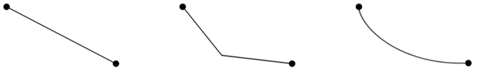
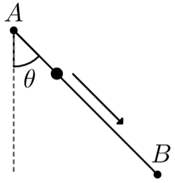
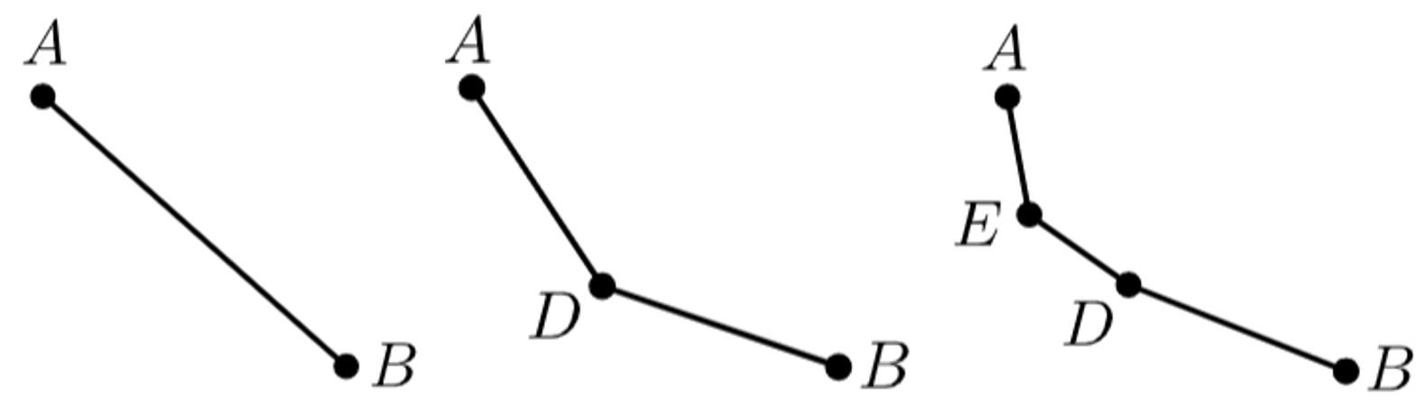
This paper aims to find the brachistochrone curve from only the basic mechanics of falling. The simplest path that the ball can take between two points is a straight line. Hence, consider the points  and
and  connected by the line
  (see Fig 2a).
 and its tangential component
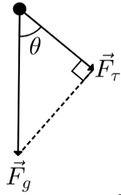
Finding the ball’s time of descent is straightforward. To begin, the ball is acted upon by the weight force , the magnitude of which is proportional to the mass of the ball:
![\[\vec{F}_g = \begin{pmatrix} 0 \ -mg \end{pmatrix} \Rightarrow F_g = mg\]](https://nhsjs.com/wp-content/ql-cache/quicklatex.com-e1b3217089f6766d5f43e06ceea10e1f_l3.png "Rendered by QuickLaTeX.com")
Where  is the magnitude of the weight force and
  is the acceleration due to gravity. Note that magnitudes of vector quantities will be represented in this paper by its symbol (e.g.
  ) without the vector arrow (e.g. ). We then find (as per Fig. 2b):
![\[F\tau = mg \cos(\theta)\]](https://nhsjs.com/wp-content/ql-cache/quicklatex.com-12ff1f7ab68305391ca3771481c3c162_l3.png "Rendered by QuickLaTeX.com")
Since the normal component of is cancelled out by reaction forces provided by the ramp (or equivalently, since the reaction forces do no work along the tangent direction for frictionless sliding),  is the net force acting on the ball. Hence, by the second law of motion, the magnitude of acceleration
  is given by:
(2.1.1) 
The direction of acceleration does not change, so only its magnitude is relevant. Hence, integrating twice with respect to elapsed time  :
:
(1) 
Both integration constants come to zero, as the magnitudes of velocity and displacement  are zero before the ball starts moving. Hence, the total time of descent is given by:
(2.1.2) 
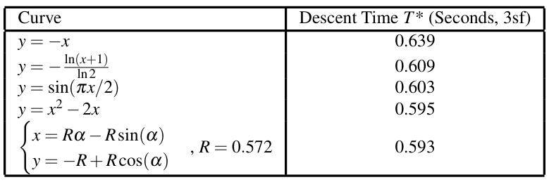
For example, if the ball falls from  to
to  , then we have:
![\[T = \sqrt{\frac{2\sqrt{2}}{9.81 \times \cos 45^\circ}} \approx 0.639 \text{ seconds}\]](https://nhsjs.com/wp-content/ql-cache/quicklatex.com-bcaa78cf0edd886fbf23c5192f6f93a2_l3.png "Rendered by QuickLaTeX.com")
Two Segments
A natural next step is to investigate a slightly more complex path, like one formed by two connected segments. To that end, add a third point  below and to the right of , forming two segments and
  .
.
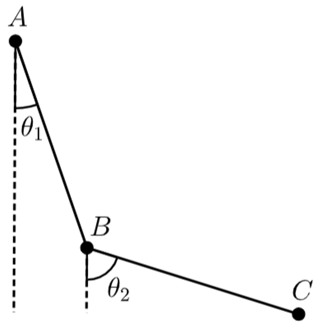
From now on, when considering multiple connected segments,  represents the angle formed against the vertical by the
  th such segment. Similarly,
  refers to the length of the th segment,
  the time of descent along it.
  has been found in the previous section, as per (2.1.2):
![\[t_1 = \sqrt{\frac{2s_1}{g \cos(\theta_1)}}\]](https://nhsjs.com/wp-content/ql-cache/quicklatex.com-7f679bbf1be1ef32d659e0125956cc24_l3.png "Rendered by QuickLaTeX.com")
The ball arrives at the second segment with a non-zero velocity (call this  ). Hence, if we ignore the first segment and define
  as the time at which the ball arrives at the second segment, then the equations of motion are:
(2) 
Where:
(2.2.1) 
Next, once the ball arrives at the second segment:
![\[s(t_2) = s_2 = \frac{1}{2} g \cos(\theta_2) t_2^2 + v_1 t_2\]](https://nhsjs.com/wp-content/ql-cache/quicklatex.com-e099904c343701af6ae6ad326e6651e8_l3.png "Rendered by QuickLaTeX.com")
Which implies a quadratic in  :
:

(3) 
Since  , there is one negative and one positive solution for . Rejecting the negative solution, we find that:
(4) 
(2.2.2) 
Consider a similar numerical example as before. Let be at , be at  , and be at
  . As such,
  ,
,  and
and  . In this case, we have
  s, which is a slightly shorter descent time than the single line segment connecting
  and
and  .
.
Speed Across Multiple Segments
As can be seen, finding time of descent becomes considerably more complex with the addition of even one more segment, since the ball arrives at the second segment with non-zero speed. Observe, however, that (by 2.2.1):
![\[\cos(\theta_1) = \frac{h_1}{s_1} \Rightarrow s_1 = \frac{h_1}{\cos(\theta_1)} \quad \therefore v_1 = \sqrt{2g \cos(\theta_1) s_1} = \sqrt{2gh_1}\]](https://nhsjs.com/wp-content/ql-cache/quicklatex.com-82df2c1444aa3ee7c8c845e2cf97086f_l3.png "Rendered by QuickLaTeX.com")
Where  is the vertical height of the first segment (see Fig. 4). Hence, depends only on , which the reader may already recognise to be equivalent to mechanical energy conservation (assuming no friction or rolling). Proving this result for any number of segments would remove the need for individually calculating the initial velocity at each junction point.
Hence, consider a ball falling along a series of connected line segments, currently falling along the th segment. Let the height through which it has fallen be  , where
  is the vertical height of the th segment.
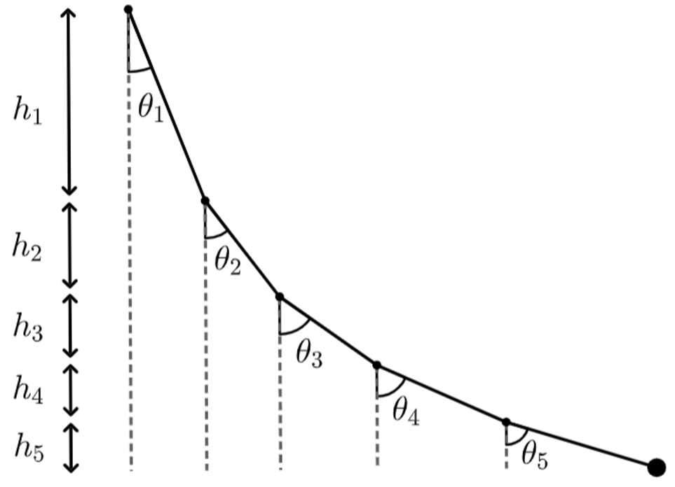
It can be shown that the speed  of the ball at the end of the th segment is dependent only on the height through which it has already fallen. More precisely:
(2.3.1) 
Proof:
The statement (2.3.1) can be proven inductively, already demonstrated for the base case  :
:
![\[v_1 = \sqrt{2gh_1}\]](https://nhsjs.com/wp-content/ql-cache/quicklatex.com-8adbe0cd48b1925118cd83125af9aa2d_l3.png "Rendered by QuickLaTeX.com")
Next, assume for induction that the case  is true. For compactness, write
  and thus
  . We now wish to prove the validity of the next case
  . Again, the acceleration
  is given by:
(2.3.2) 
As in the previous section, to find speed and distance travelled, it is most convenient to define as being the time when the ball arrives at the segment being considered (in this case the  th segment). Integrating acceleration with respect to :
(5) 
Note that, by the case, the ball has an initial velocity , i.e.  , while
  . The length
  of the
  segment is:

(6) 
Which – similar to before — is a quadratic in  . Solving for :
![\[t_{k+1} = \frac{-\sqrt{2g\Sigma_k} + \sqrt{2g\Sigma_k + 2gh_{k+1}}}{g \cos(\theta_{k+1})}\]](https://nhsjs.com/wp-content/ql-cache/quicklatex.com-64a5ca77a0cff2d88c8217f7050a9b40_l3.png "Rendered by QuickLaTeX.com")
The negative root has been rejected. Substituting this back into (2.3.2) yields:
![\[v_{k+1} = \sqrt{2g(\Sigma_k + h_{k+1})} = \sqrt{2g(h_1 + h_2 \ldots + h_k + h_{k+1})}\]](https://nhsjs.com/wp-content/ql-cache/quicklatex.com-a794b96bc3526211cfc2fe7ea6538bed_l3.png "Rendered by QuickLaTeX.com")
Recalling that  , we find that the statement is also true for
  . Hence, the statement is true for so long as it is true for . Because (2.3.1) was valid for the base case , by the principle of induction, it is true for all positive integers .
Since has not been given a value, it could, for the sake of argument, be equal to any positive real number. Hence, the statement is true continuously across every segment, not just at the endpoints. To reflect this, can be replaced by  (representing instantaneous velocity):
(2.3.3) 
Average Speed
Let the average speed of the ball falling along the th segment be  . By corollary to (2.3.3),
  is dependent only on the heights fallen:
  and
and  (with
(with  ).
).
Proof:
Again, let be the time at which the ball reaches the segment in question. The acceleration across that segment is still  , so integrating twice with respect to yields and :
(7) 
Note that  and . Next, since is the time taken to traverse :
![\[v_n = v(t_n) = g\cos(\theta_n)t_n + v_{n-1}\]](https://nhsjs.com/wp-content/ql-cache/quicklatex.com-114e840478ba59029aaaad75a91541b4_l3.png "Rendered by QuickLaTeX.com")
is given by:
![\[s_n = s(t_n) = \frac{g}{2} \cos(\theta_n)t_n^2 + v_{n-1} t_n\]](https://nhsjs.com/wp-content/ql-cache/quicklatex.com-1392467d548668d669454020f165f714_l3.png "Rendered by QuickLaTeX.com")
And hence, by definition:
![\[\bar{v}n = \frac{\text{distance}}{\text{time}} = \frac{s_n}{t_n} = \frac{g}{2} \cos(\theta_n) t_n + v{n-1} \Rightarrow \bar{v}n\]](https://nhsjs.com/wp-content/ql-cache/quicklatex.com-545365e428793b56cfbb7c3525176b4c_l3.png "Rendered by QuickLaTeX.com")
![\[= \frac{g\cos(\theta_n) t_n + 2v{n-1}}{2} = \frac{v_{n-1} + v_n}{2}\]](https://nhsjs.com/wp-content/ql-cache/quicklatex.com-f4ac8bdb6bae263d1a852582f87dcf6d_l3.png "Rendered by QuickLaTeX.com")
By (2.3.3):
(2.4.1) 
This result will be used in the next section.
Deriving A Least-Time Property
Minimizing Descent Time
Revisiting the numerical example with  ,
,  and
and  , (2.3.3) and (2.4.1) make finding descent time significantly simpler. This is since
  produces the same answer without needing to solve a quadratic:
![\[T = t_1 + t_2 = \frac{s_1}{\bar{v}_1} + \frac{s_2}{\bar{v}_2} = \frac{2 \times 0.762}{\sqrt{2g(0.7)}} + \frac{2 \times 0.762}{\sqrt{2g(0.7)} + \sqrt{2g}} \approx 0.598\text{s}\]](https://nhsjs.com/wp-content/ql-cache/quicklatex.com-8e77dad978bb0368d3c050053b4fabae_l3.png "Rendered by QuickLaTeX.com")
This observation allows us to minimise travel time by optimising the placement of . Let the vertical and horizontal distances between and be  and
and  respectively. If the positions of and are fixed – and by extension, if and are constant – what are the values of and
  (see Fig. 5) which minimise the descent time?
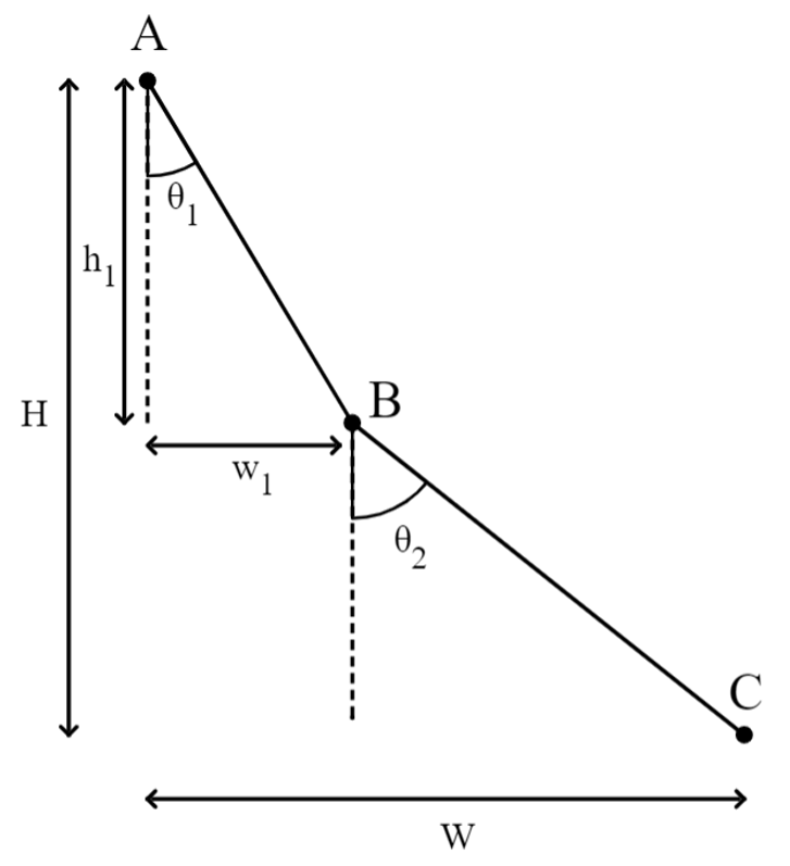
By Pythagoras, the lengths of the segments and are:
![\[\overline{AB} = \sqrt{w_1^2 + h_1^2} \qquad \overline{BC} = \sqrt{(W - w_1)^2 + (H - h_1)^2}\]](https://nhsjs.com/wp-content/ql-cache/quicklatex.com-f80b5422b41f750a3363b276a8ec62e1_l3.png "Rendered by QuickLaTeX.com")
The total travel time is simply the sum of the travel times across and :
![\[T = t_1 + t_2 = \frac{\sqrt{w_1^2 + h_1^2}}{\bar{v}_1} + \frac{\sqrt{(W - w_1)^2 + (H - h_1)^2}}{\bar{v}_2}\]](https://nhsjs.com/wp-content/ql-cache/quicklatex.com-b3ed3ece578edaf96b11b02f32563f65_l3.png "Rendered by QuickLaTeX.com")
Since is fixed, we know by (2.4.1) that the average speeds depend only on . Therefore, if is held constant, then depends on alone. As such, we can examine how the travel time is minimised by changing alone. Differentiating with respect to :
![\[\frac{dT}{dw_1} = \frac{w_1}{\bar{v}_1 \sqrt{w_1^2 + h_1^2}} - \frac{W - w_1}{\bar{v}_2 \sqrt{(W - w_1)^2 + (H - h_1)^2}} = 0\]](https://nhsjs.com/wp-content/ql-cache/quicklatex.com-13b16095ce13f6b64278d6f5fe310ae0_l3.png "Rendered by QuickLaTeX.com")
Hence, since  at minima and maxima, the following condition must upheld:
(3.1.2) 
It can be shown that is indeed minimised by analysing the second derivative. Factoring out the constant  and
and  terms and then differentiating once more with respect to :
![\[\frac{d^2T}{dw_1^2} = \frac{1}{\bar{v}_1} \times \frac{d}{dw_1} \left(\frac{w_1}{\sqrt{w_1^2 + h_1^2}}\right)- \frac{1}{\bar{v}_2} \times \frac{d}{dw_1} \left(\frac{W - w_1}{\sqrt{(W - w_1)^2 + (H - h_1)^2}}\right)\]](https://nhsjs.com/wp-content/ql-cache/quicklatex.com-626424ca995e1026a51ea8034acce8ca_l3.png "Rendered by QuickLaTeX.com")
Applying the quotient rule yields:
![\[\frac{d^2T}{dw_1^2} = \frac{h_1^2}{\bar{v}_1 (w_1^2 + h_1^2)^{3/2}} + \frac{(H - h_1)^2}{\bar{v}_1 [(W - w_1)^2 + (H - h_1)^2]^{3/2}}\]](https://nhsjs.com/wp-content/ql-cache/quicklatex.com-a0e50120de7635ed4138a68d94c19be1_l3.png "Rendered by QuickLaTeX.com")
Each term in  is a ratio of positive constants and squared distances, hence is strictly positive for all values of . Therefore,
  is concave upwards for all values of , meaning that its only stationary point is a minimum which occurs when:
![\[\frac{w_1}{\bar{v}_1 \sqrt{w_1^2 + h_1^2}} = \frac{W - w_1}{\bar{v}_2 \sqrt{(W - w_1)^2 + (H - h_1)^2}}\]](https://nhsjs.com/wp-content/ql-cache/quicklatex.com-eca4780d578b302304d870a0fa1dffff_l3.png "Rendered by QuickLaTeX.com")
Snell’s Law
We have found that descent time is minimised when  , which is an unwieldy result. Since
  , this can be rewritten as:
![\[\frac{w_1}{\bar{v}_1 \sqrt{w_1^2 + h_1^2}} = \frac{\sin(\theta_1)}{\bar{v}_1} = \frac{W - w_1}{\bar{v}_2 \sqrt{(W - w_1)^2 + (H - h_1)^2}} = \frac{\sin(\theta_2)}{\bar{v}_2}\]](https://nhsjs.com/wp-content/ql-cache/quicklatex.com-108136daf675d95a30880b3d1fd38a42_l3.png "Rendered by QuickLaTeX.com")
Next, it has been shown that there is only one value of which minimises . As a result, for constant , point is `fixed’. In that case, therefore, the angles  and
and  are constant (as are
  and
and  by extension). Let
  represent a constant term ( in fact scales the radius of the cycloid), meaning the time-minimising condition can be rewritten as:
(3.2.1) 
This result is well-known in physics as Snell’s law, which describes the path that light will take as it moves through different media. Light travels through different materials at different (but constant) velocities and will always take the least-time path, so the motion of light rays (as first noticed by Bernoulli in his optical-mechanical analogy18,19 and subsequently re-applied by others20 is directly applicable to this optimisation problem.
Generalising To Segments
The time-minimising property has been proven directly before for two segments ( and ), but can be generalised to two points connected by segments. In other words, for an object falling down connected segments which each have a fixed vertical height, the condition which minimises the total travel time  is:
is:
(3.3.1) 
Proof:
By (2.3.3), the vertical heights  being fixed means that the initial speeds
  are also fixed, as are the average speeds
  . Therefore, varying the width
  of the th segment will only affect the travel time across that particular segment. This is key.
As such, assume that the segments form the time-minimising path:
- If and
 are such that
  , then
  can be decreased while all other descent times stay the same, which would decrease the total travel time . Contradiction. Hence,
  .
. - If and
 are such that
  , then
  can be decreased, which would decrease the value of . Contradiction. Hence,
  .
. 
- If
 and are such that
  , then
  can be decreased, which would decrease the value of . Contradiction. Hence,
  .
.
Hence, by transitivity, we arrive at the generalisation:
![\[\frac{\sin(\theta_1)}{\bar{v}_1} = \frac{\sin(\theta_2)}{\bar{v}_2} \ldots = \frac{\sin(\theta_n)}{\bar{v}_n} = k\]](https://nhsjs.com/wp-content/ql-cache/quicklatex.com-da99d2fb1f2c825e9ecb8feda4bbc6cd_l3.png "Rendered by QuickLaTeX.com")
Finding The Brachistochrone
‘Smooth’ Curve
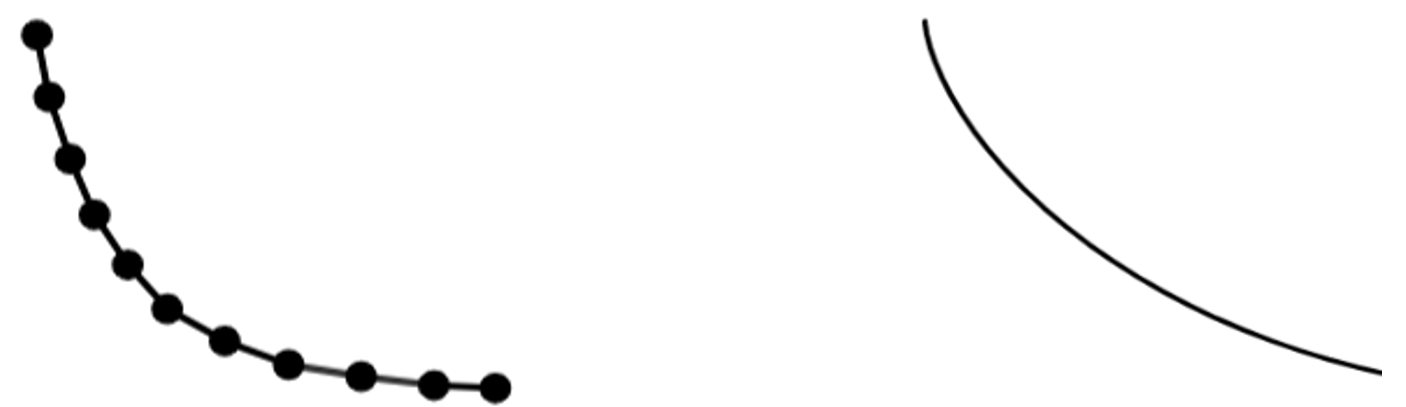
So far, the time-minimising condition has been found for a mass travelling down connected line segments. Such a path is not smooth, as the mass experiences an abrupt change in direction at the boundary between each segment.
However, since speed depends only on height fallen, it can be argued that the brachistochrone is a smooth curve, or at least approximates one. Considering two points ( and ), observe that:
- The descent time between and (call this
 ) can be decreased by adding an intermediate point () between and , so long as the placement of fulfils (3.3.1). This can be done without affecting any other descent time because the relative heights of the other points are unchanged (and thus the average speed along them too).
 - Similarly,
 can be decreased by adding another point (
 ) between and , such that the placement of
  and
and  fulfils (3.3.1).
 - Then,
 can be decreased by adding another point between and , and so on.
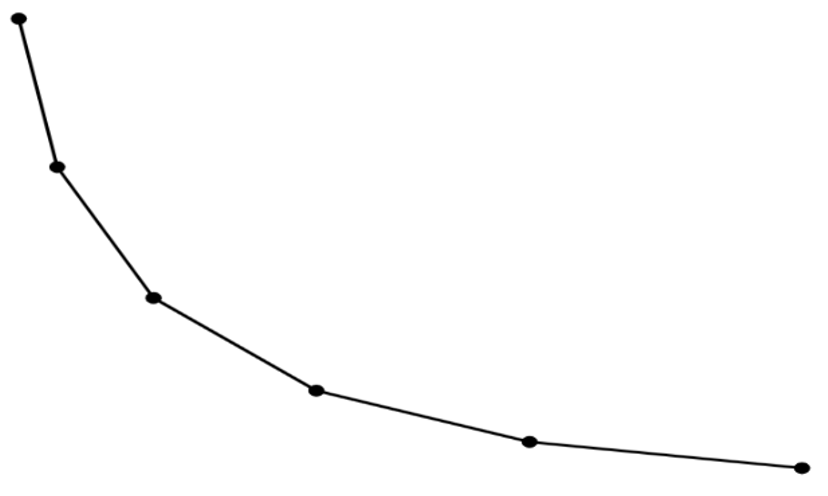
More intermediate points can added until the length of each connecting segment approaches zero. This path (approaching `infinitely’ many points) would intuitively be the brachistochrone, since no more points can be added to decrease travel time further.
Strictly speaking, this argument is only heuristic, and should not be construed as a rigorous proof of the brachistochrone’s smoothness (since `smoothness’ has a specific definition within real analysis). As noted in the introduction, a fully rigorous solution to the brachistochrone problem would require variational calculus, which is beyond the scope of this paper.
However, this argument demonstrates the need for the length of each segment to approach zero – implying that the curve eventually becomes infinitely differentiable. In addition, it acts as a useful intuition for how the time-minimising curve may be found via integration.
The Brachistochrone Integral
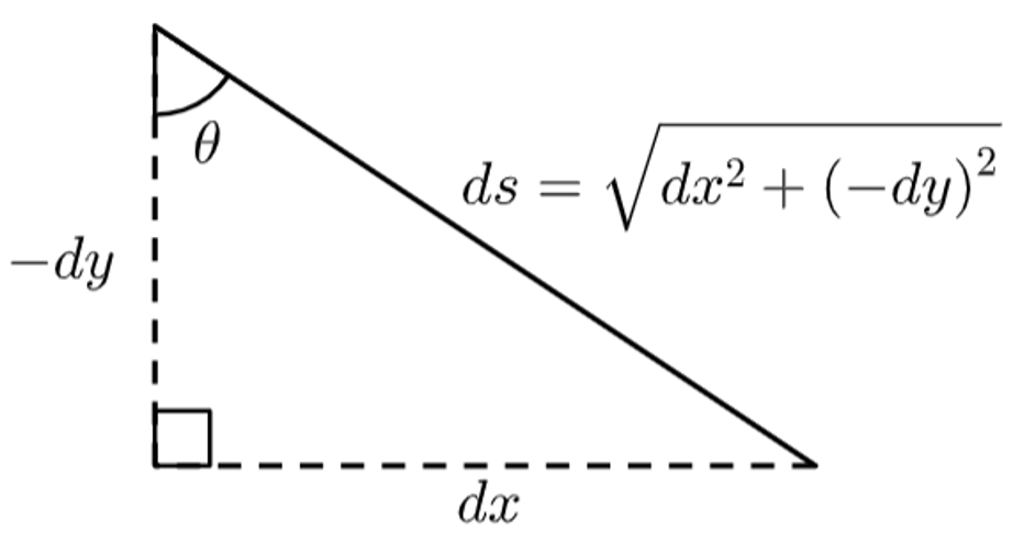
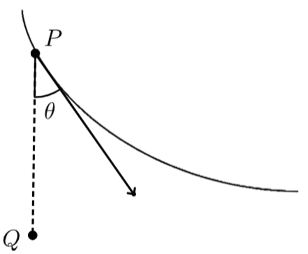
Consider an infinitesimally short segment  on this `smooth’ time-minimising curve, which forms an angle
  against the -axis. As per Fig. 8, a mass falling along would travel vertically and horizontally by the distances
  and
and  respectively (note the negative sign on because the ball is falling downwards).
being infinitesimally short means that the ball’s average speed is essentially equal to its instantaneous speed, the change in height tends towards zero. By (2.4.1):
![\[\bar{v}n = \lim{h_n \to 0} \frac{\sqrt{2g(\Sigma_n - h_n)} + \sqrt{2g\Sigma_n}}{2} = \sqrt{2g\Sigma_n} = v\]](https://nhsjs.com/wp-content/ql-cache/quicklatex.com-a91c1bb499be567e7c65dd957f6e40dc_l3.png "Rendered by QuickLaTeX.com")
Note that  exactly, since acceleration becomes constant in the limit
  . Hence, since (3.3.1) is fulfilled instantaneously across the brachistochrone, rewrite it as:
(4.2.1) 
By Pythagoras,  can be rewritten:
![\[\frac{dx}{\sqrt{dx^2 + (-dy)^2}} = kv\]](https://nhsjs.com/wp-content/ql-cache/quicklatex.com-15207a4e38349ffd6ac59af6bcf763e5_l3.png "Rendered by QuickLaTeX.com")
Rearranging algebraically, this can be interpreted as a differential equation:
(8) 
(4.2.2) 
Recalling (2.3.3), the velocity of the ball depends only on the height through which it has already fallen. Again, since the ball begins at the point , the vertical distance fallen is simply the negative -coordinate, or  . By (2.3.3):
![\[v = \sqrt{2g(h_1 + h_2 \ldots + h_n + h_{n+1})} = \sqrt{2g(-y)}\]](https://nhsjs.com/wp-content/ql-cache/quicklatex.com-d180c8de38899dba8b1508d26a668dfd_l3.png "Rendered by QuickLaTeX.com")
(4.2.3) 
Which is equivalent to conservation of mechanical energy (assuming no friction or rolling). This can be substituted back into (4.2.2):
(4.2.4) 
The constant  has been introduced for convenience. This derivative form, however, does not provide very much insight into the curve it describes. As such, we integrate with respect to to find the Cartesian form.
![\[x = \int -\sqrt{\frac{-Cy}{1 + Cy}} \, dy = -\int \sqrt{\frac{-Cy}{1 + Cy}} \, dy\]](https://nhsjs.com/wp-content/ql-cache/quicklatex.com-9acfc084731ead3273f52729582a46d5_l3.png "Rendered by QuickLaTeX.com")
Evaluating this integral is tedious. First, the integrand may be manipulated with the substitution:
![\[u = \sqrt{\frac{-Cy}{Cy + 1}} \Rightarrow y = -\frac{u^2}{C(u^2 + 1)} \Rightarrow dy = -\frac{2u}{C(u^2 + 1)^2} \, du\]](https://nhsjs.com/wp-content/ql-cache/quicklatex.com-96c726c0dc03ab89d3815b65d80756d6_l3.png "Rendered by QuickLaTeX.com")
Hence, by the chain rule:
(9) 
The remaining integral  is best evaluated using a trigonometric substitution:
![\[z = \arctan(u) \Rightarrow du = \sec^2(z) \, dz\]](https://nhsjs.com/wp-content/ql-cache/quicklatex.com-398a786bc0aecc1e91031bc954189252_l3.png "Rendered by QuickLaTeX.com")
Which yields:
(10) 
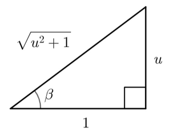
The  substitution can be undone by noting that:
![\[\sin(\arctan(u)) = \frac{u}{\sqrt{u^2 + 1}} \qquad \text{and} \qquad \sin(\arctan(u)) = \frac{1}{\sqrt{u^2 + 1}}\]](https://nhsjs.com/wp-content/ql-cache/quicklatex.com-1bea0308a06c45225c4abeb1206b7435_l3.png "Rendered by QuickLaTeX.com")
 and
and  .
.These relations can be proven efficiently by constructing a right triangle with side lengths  ,
,  and . From Fig. 9, observe that:
![\[\sin(\arctan(u)) = \sin(\varphi) = \frac{u}{\sqrt{u^2 + 1}}\]](https://nhsjs.com/wp-content/ql-cache/quicklatex.com-6c6dd6eb64af9a15ecd2e469c37ae7e5_l3.png "Rendered by QuickLaTeX.com")
![\[\qquad \text{and} \qquad \cos(\arctan(u)) = \cos(\varphi) = \frac{1}{\sqrt{u^2 + 1}}\]](https://nhsjs.com/wp-content/ql-cache/quicklatex.com-cf4988c8cf68617e68e6a65617c31f73_l3.png "Rendered by QuickLaTeX.com")
As such, undoing the substitution yields:
![\[\frac{1}{2} \sin(z)\cos(z) + \frac{z}{2} = \frac{u}{2(u^2 + 1)} + \frac{1}{2} \arctan(u)\]](https://nhsjs.com/wp-content/ql-cache/quicklatex.com-b330a3e2cd8d23ec8c4dbd6dde19d6aa_l3.png "Rendered by QuickLaTeX.com")
Finally, putting everything together and undoing the substitution:
![\[x &= \frac{2}{C} \left(\arctan(u) - \int \frac{1}{(u^2 + 1)^2} \, du\right) = \frac{1}{C} \arctan(u) - \frac{1}{C} \times \frac{u}{(u^2 + 1)}\]](https://nhsjs.com/wp-content/ql-cache/quicklatex.com-8f4296b34f60a09cb3ffe4333d33d777_l3.png "Rendered by QuickLaTeX.com")
![\[&\Rightarrow x = \frac{1}{C} \arctan\left(\sqrt{\frac{-Cy}{Cy + 1}}\right) - \frac{1}{C} \times \frac{\left(\sqrt{\frac{-Cy}{Cy + 1}}\right)}{\left(1 - \frac{Cy}{Cy + 1}\right)}\]](https://nhsjs.com/wp-content/ql-cache/quicklatex.com-a829a9ccd8672ac3099713e70cc48b99_l3.png "Rendered by QuickLaTeX.com")
![\[&= \frac{1}{C} \arctan\left(\sqrt{\frac{-Cy}{Cy + 1}}\right) - \frac{1}{C} \times \frac{\left(\sqrt{\frac{-Cy}{Cy + 1}}\right)}{\left(\frac{1}{Cy + 1}\right)}\]](https://nhsjs.com/wp-content/ql-cache/quicklatex.com-4440ef22d26e7a63236b1120686c7af4_l3.png "Rendered by QuickLaTeX.com")
The curve begins at . Hence,  and the constant of integration comes to zero:
(4.2.5) 
This is the explicit solution to (4.2.2). Since it obeys the `instantaneous’ least-time condition (4.2.1), it must represent the least-time curve, i.e. the brachistochrone.
Parametric Representation
The arctangent term in (4.2.5) makes algebraic manipulation impractically complex. As such, representation using parametric equations is more elegant. Let  , which would eliminate the nested square root via substitution (
 is a parameterising variable whose geometric meaning will be demonstrated later). Making the subject:
![\[\tan^2(\beta) = \frac{-Cy}{1 + Cy} \Rightarrow -\tan^2(\beta) = Cy(\tan^2(\beta) + 1)\]](https://nhsjs.com/wp-content/ql-cache/quicklatex.com-bd62ee8c361b70666413872fca4542e4_l3.png "Rendered by QuickLaTeX.com")
![\[\Rightarrow y = -\frac{1}{C} \times \frac{\tan^2(\beta)}{\tan^2(\beta) + 1}\]](https://nhsjs.com/wp-content/ql-cache/quicklatex.com-88aa44db4282ab933daa82ab348ddf0c_l3.png "Rendered by QuickLaTeX.com")
Noting that  :
:
![\[y = -\frac{1}{C} \times \frac{\tan^2(\beta)}{\tan^2(\beta) + 1} = -\frac{1}{C} \times \frac{\left(\frac{\sin^2(\beta)}{\cos^2(\beta)}\right)}{\left(\frac{\sin^2(\varphi) + \cos^2(\beta)}{\cos^2(\beta)}\right)} = -\frac{1}{C} \sin^2(\beta)\]](https://nhsjs.com/wp-content/ql-cache/quicklatex.com-e9e64ec87eed1e17b38e4c62d85cd83b_l3.png "Rendered by QuickLaTeX.com")
(4.3.1) 
Similarly, rearranging to make the subject:
(4.3.2) 
Finally, introducing the constant  and changing the parameterising variable to
  yields a simpler set of equations than (4.3.1) and (4.3.2):
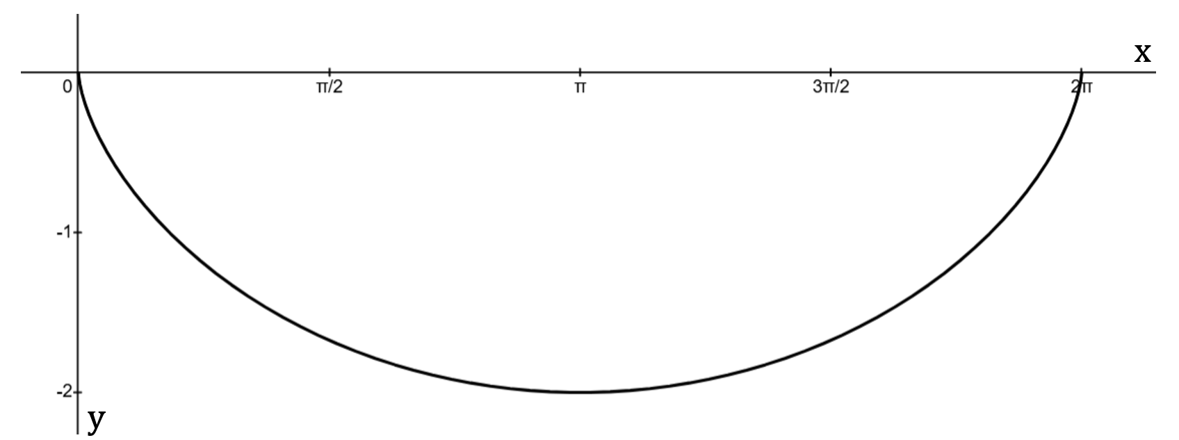
![\[x = R\alpha - R\sin(\alpha)\]](https://nhsjs.com/wp-content/ql-cache/quicklatex.com-07d68b3bc4c805e99ae642f5f24b5412_l3.png "Rendered by QuickLaTeX.com")
![\[y = -R + R\cos(\alpha)\]](https://nhsjs.com/wp-content/ql-cache/quicklatex.com-426b3a3deacaae846858d979d51a4fb9_l3.png "Rendered by QuickLaTeX.com")
These are the standard parametric equations for the inverted cycloid traced by a circle of radius  whose centre rolls along the line
  .
.
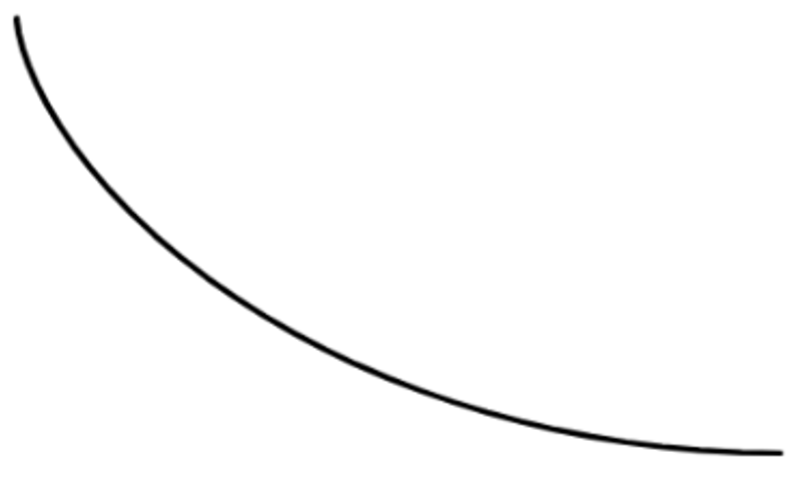
As shown below in Fig. 10, observe how the brachistochrone starts steep, before flattening out. This can be understood intuitively as arising from a tradeoff between acceleration (requiring a steep gradient), and then covering horizontal distance (requiring a shallow / flat gradient).
 and
and 
The Cycloid
(4.3.3) Is the set of parametric equations which describe the brachistochrone, found using integration. These equations in fact describe a cycloid – the locus of a point on the circumference of a circle which rolls without slipping at a constant speed.
Proof:
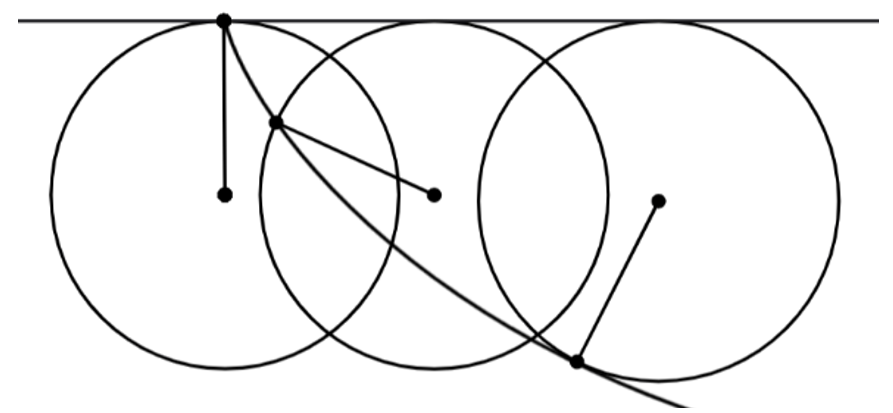
Consider a generating circle with radius , rolling with a constant speed in the positive -direction (rightwards). Let  be the point on its circumference which begins at the origin , such that the path traced out by is a cycloid. Suppose then that the circle rolls for an arbitrary amount of time, with the centre of the circle travelling through through the length
  and
and  being the (counterclockwise) angle through which has turned from rest.
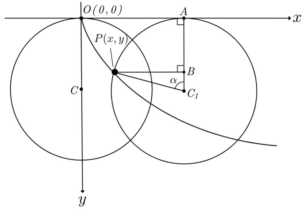
Let and be points on the -axis and  respectively, such that
  and
and  . Since
  , the -position of is given by:
![\[y = -\overline{AC_1} + \overline{BC_1} = -R + R\cos(\alpha)\]](https://nhsjs.com/wp-content/ql-cache/quicklatex.com-3fbcca020e9c9254cc79ae8de6e3777f_l3.png "Rendered by QuickLaTeX.com")
The length (and by extension ‘s -position) are not readily apparent. However, rolling without slipping means that the circle’s centre must travel a distance equal to the arclength swept out by . In other words,  . Hence:
![\[x = \overline{CC_1} - \overline{PB} = R\alpha - R\sin(\alpha)\]](https://nhsjs.com/wp-content/ql-cache/quicklatex.com-4e74d1e56cbcc8e43cf6369a6d3753a1_l3.png "Rendered by QuickLaTeX.com")
Fig. 12 depicts an acute . For the sake of completeness, however, the same result may be obtained for any  , with the process being repeated almost verbatim.
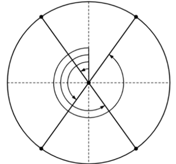 ) swept through by P is greater than
![\[&\text{If } 0 \leq \alpha \leq \tfrac{\pi}{2}, \text{ then } x = R \alpha - R \sin(\alpha)\]](https://nhsjs.com/wp-content/ql-cache/quicklatex.com-01651f7e41958cb57f734e9bf216aecc_l3.png "Rendered by QuickLaTeX.com")
![\[\text{ and } y = -R + R \cos(\alpha) \quad \text{(as before)}\]](https://nhsjs.com/wp-content/ql-cache/quicklatex.com-411e28c8606e1dc2f087373243ceadb5_l3.png "Rendered by QuickLaTeX.com")
![\[&\text{If } \tfrac{\pi}{2} \leq \alpha \leq \pi, \; x = R \alpha - R \cos!\left(\alpha - \tfrac{\pi}{2}\right)\]](https://nhsjs.com/wp-content/ql-cache/quicklatex.com-e452a8de383457f6884a06c49b8a37eb_l3.png "Rendered by QuickLaTeX.com")
![\[= R \alpha - R \sin(\alpha) \text{ and } y = -R - R \sin!\left(\alpha - \tfrac{\pi}{2}\right)\]](https://nhsjs.com/wp-content/ql-cache/quicklatex.com-b7713d1bebd59b461ddea721dffe302c_l3.png "Rendered by QuickLaTeX.com")
![\[= -R + R \cos(\alpha)\]](https://nhsjs.com/wp-content/ql-cache/quicklatex.com-f1ea870376b979c5c591bffaeb90b4bc_l3.png "Rendered by QuickLaTeX.com")
![\[&\text{If } \pi \leq \alpha \leq \tfrac{3\pi}{2}, \; x = R \alpha + R \sin(\alpha - \pi)\]](https://nhsjs.com/wp-content/ql-cache/quicklatex.com-af7583e561365a4d0b2bfea6596637d8_l3.png "Rendered by QuickLaTeX.com")
![\[= R \alpha - R \sin(\alpha) \text{ and } y = -R - R \cos(\alpha - \pi)\]](https://nhsjs.com/wp-content/ql-cache/quicklatex.com-8413123757e0c9fa789bafb673fd4d5f_l3.png "Rendered by QuickLaTeX.com")
![\[&\text{If } \tfrac{3\pi}{2} \leq \alpha \leq 2\pi, \; x = R \alpha +\]](https://nhsjs.com/wp-content/ql-cache/quicklatex.com-cea79a065a2641b8d44204063eb5ee21_l3.png "Rendered by QuickLaTeX.com")
![\[R \cos!\left(\alpha - \tfrac{3\pi}{2}\right)\]](https://nhsjs.com/wp-content/ql-cache/quicklatex.com-56b55cd276f6c3a528c5c7bd694024d7_l3.png "Rendered by QuickLaTeX.com")
![\[= R \alpha - R \sin(\alpha) \text{ and } y = -R + R \sin!\left(\alpha - \tfrac{3\pi}{2}\right)\]](https://nhsjs.com/wp-content/ql-cache/quicklatex.com-fab7b98ddb4f2e63066dccb73a3e38c9_l3.png "Rendered by QuickLaTeX.com")
Thus, for a generating circle with radius , the position of is given by 
 , which exactly matches the parametric equations derived in (4.3.3). The shape of the brachistochrone, therefore, is that of an inverted cycloid.
Boundary Conditions / Completeness
Though important for completeness, fully accounting for the boundary conditions (that is, finding how the generating circle radius depends on the start and endpoints) is beyond the scope of this paper. For example, forcing the cycloid to pass through the earlier points and yields:

(11) 
 is transcendental, while
  simply means the brachistochrone starts from the `cusp’ of the cycloid. Hence, in the case where only start and end points are known (as Bernoulli’s original problem statement suggests), cannot be found purely algebraically21 (except when the end point is at the same height as the starting point). Rigorously confirming that this time-minimising value of is unique (and actually time-minimising) is similarly beyond the scope of this paper, requiring complex variational methods22,23,24.
Nonetheless, suitable values of R can still be found numerically, demonstrating the brachistochrone property of the cycloid. For example, considering curves which begin at (0,0) and end at (1,-1):
A Geometric Approach (Comparison)
Setup and Motivation
In the previous section, a cycloidal path was shown to instantaneously fulfil the least-time condition  identified in (4.2.1). However, the approach taken — forming and then solving a differential equation — was highly mechanical. It can in fact be confirmed more elegantly that the cycloid obeys at every point through a purely geometric method7.
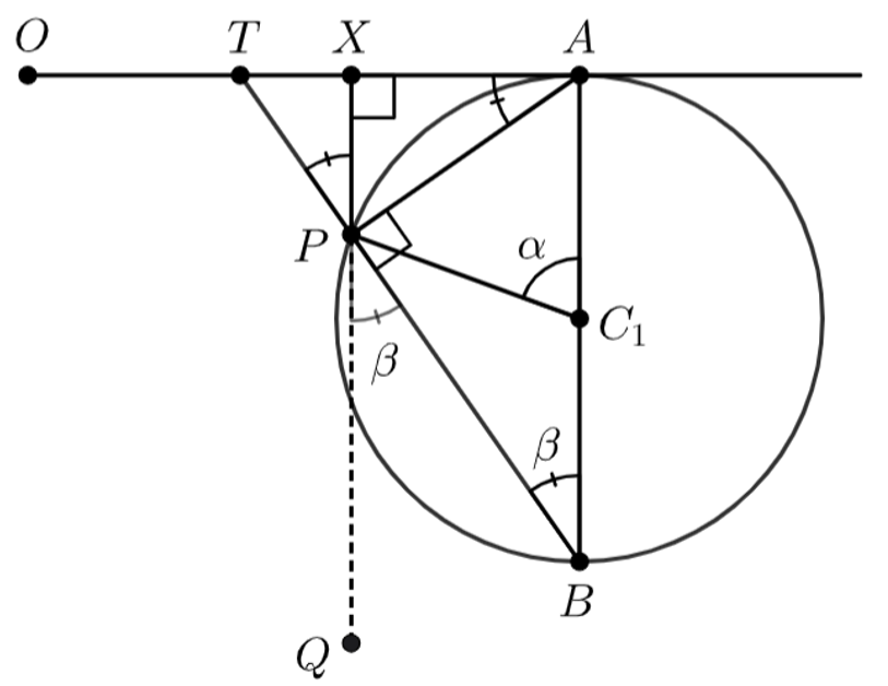
As before, consider some point on the cycloid, which lies on the circumference of its generating circle, currently centred on  (the cycloid is not shown in Fig. 14a to prevent clutter). Construct a line such that it forms the vertical diameter of the generating circle, with
  . By Thales’ theorem,
  is a right triangle, with
  .
.
Next, extend  until it reaches
  at and let
  be the vertical height fallen by .
  , so by corresponding angles,
  , while
  by alternating angles. Noting further that angle at centre
  at circumference:
![\[A\widehat{C}_1P = \alpha = 2X\widehat{P}T = 2A\widehat{B}T = 2\beta\]](https://nhsjs.com/wp-content/ql-cache/quicklatex.com-3fd1cd1bf3cb5c1c5c26c9596b26110d_l3.png "Rendered by QuickLaTeX.com")
As per the substitution . The key to this approach, then, is that if  is the tangent to the cycloid at , then
  , which in turn allows for confirmation of the condition
  by analysing the geometry of the triangle
  .
.
Tangency Of 
The author of7 notes that the tangent to the cycloid always passes through the bottom of the generating circle, or that (as per Fig. 14a) is the tangent to the cycloid at .
Proof:
Recalling (4.3.3), the position of is given by:
Hence, by the chain rule, the gradient of the cycloid at is:
![\[\frac{dy}{dx} = \frac{dy}{d\alpha} \times \frac{d\alpha}{dx} = \frac{-R\sin(\alpha)}{R - R\cos(\alpha)} = \frac{-\sin(\alpha)}{1 - \cos(\alpha)} = \frac{-\sin(2\theta)}{1 - \cos(2\theta)}\]](https://nhsjs.com/wp-content/ql-cache/quicklatex.com-f2daae9e3f7ee848930fa462ba9f6fe1_l3.png "Rendered by QuickLaTeX.com")
![\[= \text{RHS}_1\]](https://nhsjs.com/wp-content/ql-cache/quicklatex.com-e2b1020d5ebaed31e8d3f35806285680_l3.png "Rendered by QuickLaTeX.com")
Observe that if is the tangent to the cycloid, then:
![\[\frac{dy}{dx} = \frac{\text{Rise}}{\text{Run}} = -\frac{\overline{AB}}{\overline{TA}} = -\tan(A\widehat{T}B) = -\tan(90^\circ - \theta) = \text{RHS}_2\]](https://nhsjs.com/wp-content/ql-cache/quicklatex.com-f28c9eb8dade59730b1059bb6da9ee1e_l3.png "Rendered by QuickLaTeX.com")
Simplifying the  and
and  further:
(12) 
![\[\text{RHS}_1 = \text{RHS}_2 \Rightarrow \frac{dy}{dx} = -\tan(A\widehat{T}B)\]](https://nhsjs.com/wp-content/ql-cache/quicklatex.com-f3e75e0f31faa1ad310b8a7b3c476d72_l3.png "Rendered by QuickLaTeX.com")
Therefore, is the tangent to the cycloid at , meaning is in fact the same angle as .
Fulfilling The Least-Time Condition
Since , showing the cycloid’s fulfilment of the condition can be done through basic angle-chasing and geometry.
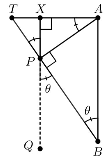
 TAP
TAPBecause  and
and  are both right triangles, we have:
![\[X\widehat{A}P = 180^\circ - (A\widehat{T}P + 90^\circ) = 180^\circ - (90^\circ - \theta + 90^\circ) = \theta\]](https://nhsjs.com/wp-content/ql-cache/quicklatex.com-2b7c113a18ac364d1a18fbf955b65bc8_l3.png "Rendered by QuickLaTeX.com")
Hence, since  is the vertical height fallen by the ball:
![\[\sin(X\widehat{A}P) = \sin(\theta) = \frac{\overline{XP}}{\overline{AP}} \Rightarrow \overline{AP} = \frac{\overline{XP}}{\sin(\theta)} = \frac{-y}{\sin(\theta)}\]](https://nhsjs.com/wp-content/ql-cache/quicklatex.com-85f2bd9aedbd2d781daa7ac447bde4fc_l3.png "Rendered by QuickLaTeX.com")
Similarly, for  :
:
![\[\sin(A\widehat{B}T) = \sin(\theta) = \frac{\overline{AP}}{\overline{AB}} = \frac{-y}{2R\sin(\theta)} \Rightarrow \frac{\sin^2(\theta)}{-y} = \frac{1}{2R}\]](https://nhsjs.com/wp-content/ql-cache/quicklatex.com-f9ed22bebce421a6206bd7d8d70153e1_l3.png "Rendered by QuickLaTeX.com")
Recalling (4.2.3) and undoing the substitutions made in the previous section:
This yields:
![\[\frac{\sin^2(\theta)}{-y} = \frac{2g\sin^2(\theta)}{v^2} = \frac{1}{2R} \Rightarrow \frac{\sin^2(\theta)}{v^2} = \frac{1}{4gR}\]](https://nhsjs.com/wp-content/ql-cache/quicklatex.com-afdd505064a296947c7499a8c6f547f2_l3.png "Rendered by QuickLaTeX.com")
![\[\therefore \frac{\sin(\theta)}{v} = \frac{1}{2\sqrt{gR}} = k\]](https://nhsjs.com/wp-content/ql-cache/quicklatex.com-8cce67a61d8205583483e73284d33395_l3.png "Rendered by QuickLaTeX.com")
By the geometry of the tangent and generating circle, therefore, the least-time condition identified in (4.2.1) is satisfied at every point along the inverted cycloid — which has been demonstrated without resorting to tedious integration.
Conclusion
Initial investigation of motion along one and two line segments provided the insights necessary to minimise descent time along connected lines. In the continuous limit, this condition implied a differential equation, the solution of which describes an inverted cycloid. Geometric analysis7 confirmed this property of the cycloid, and had the advantage of requiring less tedious algebra and the assumption of `smoothness’ — though, without the machinery of variational calculus, neither approach can incorporate the initial and final boundary conditions.
Therefore, for a point mass, the curve which minimises the time of descent between two points is an inverted cycloid, which can be represented parametrically by the equations
which have derived in an entirely `ground-up’ manner, starting with basic mechanics and proceeding using methods — employing an inductive proof, contradiction, simple integration methods, and angle-chasing in the geometric approach — which should be entirely familiar to high school students.
References
- J. Bernoulli. Solutio problematis a se in Actis 1696, propositi, de invenienda linea brachystochrona. Acta Eruditorum. pg. 206–211, 1697 [↩] [↩]
- M. A. Lerma. A simple derivation of the equation for the brachistochrone curve. Northwestern University, 2023. [↩]
- G. Lawlor. A new minimization proof for the brachistochrone. The American Mathematical Monthly. Vol 103, pg. 242–249, 1996 [↩]
- H. Erlichson, Johann Bernoulli’s brachistochrone solution using Fermat’s principle of least time, European Journal of Physics, Vol. 20, pg. 299–304, 1999. [↩]
- R. T. Boute. The brachistochrone problem solved geometrically: a very elementary approach. Mathematics Magazine. Vol 85, pg. 193–199, 2012 [↩] [↩]
- G. Brookfield. Yet another elementary solution of the brachistochrone problem. Mathematics Magazine. Vol 83, pg. 104–110, 2010 [↩]
- S. Hayes, The Brachistochrone problem, M500 Society, Vol 291, pg. 1–7, 2019. [↩] [↩] [↩] [↩]
- A. Tan, A. K. Chilvery, M. Dokhanian. Dynamical variables in brachistochrone problem. Lat. Am. J. Phys. Educ. Vol 6, pg. 196–199, 2012. [↩]
- Y. Nishiyama. The brachistochrone curve: the problem of quickest descent. International Journal of Pure and Applied Mathematics. Vol. 82, pg. 409–419, 2013. [↩] [↩]
- S. Mertens, S. Mingramm. Brachistochrones with loose ends. European Journal of Physics. Vol 29, pg. 795–802, 2008. [↩]
- S. R. Bistafa. Euler’s navigation variational problem. Euleriana. Vol 2, pg. 131–142, 2022. [↩]
- G. L. Silva, M. A. D. Pereira. Infinite horizon problems in the calculus of variations: the role of transformations with an application to the brachistochrone problem. Set-Valued and Variational Analysis. Vol 27, pg. 201–224, 2018 [↩]
- C. Criado, N. Álamo. Solving the brachistochrone and other variational problems with soap films. American Journal of Physics. Vol 78, pg. 1400–1405, 2010. [↩]
- S. Gómez-Aíza, R. W. Gómez, V. Marquina. A simplified approach to the brachistochrone problem. European Journal of Physics. Vol 27, pg. 1091–1098, 2006. [↩]
- M. A. Lerma. A simple derivation of the equation for the brachistochrone curve. Northwestern University, 2023 [↩]
- H. Erlichson, Johann Bernoulli’s brachistochrone solution using Fermat’s principle of least time, European Journal of Physics, Vol. 20, pg. 299–304, 1999 [↩]
- G. Lawlor. A new minimization proof for the brachistochrone. The American Mathematical Monthly. Vol 103, pg. 242–249, 1996. [↩]
- H. W. Broer. Bernoulli’s light ray solution of the brachistochrone problem through Hamilton’s eyes. International Journal of Bifurcation and Chaos. Vol 24, 2014. [↩]
- H. J. Sussmann, J. C. Willems. Contemporary trends in nonlinear geometric control theory and its applications, pg. 113–166, 2002. [↩]
- K. Kim, J.-H. Ee, K. Kim, U.-R. Kim, J. Lee. Mechanical Snell’s law. Journal of the Korean Physical Society. Vol 76, pg. 281–290, 2020. [↩]
- M. G. Katz, D. M. Schaps, S. Shnider. Almost equal: the method of adequality from Diophantus to Fermat and beyond. Perspectives on Science. Vol 21, pg. 283–314, 2012. [↩]
- P. G. Ciarlet, C. Mardare. On the brachistochrone problem. Communications in Mathematical Analysis and Applications. Vol 1, pg. 213–240, 2022. [↩]
- J. L. Troutman. Variational calculus and optimal control: Optimization with elementary convexity, 2nd ed. pg. 66–68, 1996. [↩]
- P. Kosmol. Bemerkungen zur brachistochrone. Abhandlungen aus dem Mathematischen Seminar der Universität Hamburg. Vol 54, pg. 91–94, 1984. [↩]


