The Application of Natural Language Processing Techniques for Detecting Bias and Toxicity in Journalism and Mpox Related News Media

Abstract

This study leverages Natural Language Processing techniques to automate the process of identifying various kinds of bias in journalism. Specifically, our models predict the type of bias (e.g. framing, confirmation), level of bias (neutral, slightly, highly biased) and the presence of toxicity within a corpus of news articles related to a multitude of topics. For this purpose, we leverage three machine learning models of varying complexity: logistic regression, decision trees and Bidirectional Encoder Representations from Transformers (BERT), a state-of-the-art transformer-based model, pre-trained for NLP tasks. We assess the models’ ability to determine keywords representative of a given type and level of bias, thus ensuring interpretability. First, we devise a hypothesis based on the most common words and phrases associated with each label (e.g., keywords corresponding to a news article categorized as health-related, slightly biased, and toxic). We assess the hypothesis and evaluate the models’ performance using macro-F1 score as the primary metric and inspecting SHapley Additive exPlanations (SHAP) values, pointing to specific keywords for each predicted class. We find that BERT demonstrates optimal performance (47.9%), providing an improvement over simpler models; specifically, BERT is adept at identifying confirmation and health-related bias. Lastly, we apply BERT to articles related to the Mpox outbreak. The model categorized most content as health-related but reveals varying bias levels depending on framing and tone. This showcases its potential as a groundbreaking editorial tool that equips journalists to refine content for objectivity before publication.

Introduction

Over the past decade, the rapid evolution of news media has transformed how information is spread worldwide, enabling an unprecedented flow of new perspectives. Despite the positive impact of news media platforms, they have also contributed to the widespread misinformation and disinformation, which amplifies bias and toxicity. Misinformation refers to false or inaccurate information that is shared without the intent to deceive. Disinformation, on the other hand, refers to false information that is deliberately created and spread to mislead. The vast amount of information and opinionated content obscures the distinction between verified facts and subjective viewpoints, making it difficult for laypeople to tell which is which. This emphasizes the need for accurate tools to detect bias and toxicity 

To this end, our work applies Natural Language Processing (NLP) techniques to analyze a dataset of news article texts, focusing on patterns in language that hint at bias and emotional undertones. By being trained on articles published in various news outlets, the NLP model can recognize and categorize different types of bias and toxic language. We optimize three different machine learning models: logistic regression, decision trees, and Bidirectional Encoder Representations from Transformers (BERT), a cutting-edge large language model specifically pre-trained for NLP tasks. We assess the models’ ability to determine keywords which are representative of a given type and level of bias, thus ensuring that the models are interpretable. We first formulate a hypothesis by identifying the most frequent words and phrases linked to each label (e.g., keywords corresponding to articles classified as health-related, slightly biased, or toxic). To evaluate this hypothesis, we apply our models to the dataset and measure their performance by assessing macro-F1 score¹, as our primary metric. We further examine model interpretability by inspecting the SHapley Additive exPlanations or SHAP² which highlight the specific keywords influencing each predicted class. Lastly, we apply BERT to an additional set of articles related to Mpox and conduct a qualitative assessment of the predicted labels. Due to computational resource limitations, only the logistic regression model was trained on the full dataset of 871,876 articles, while the more complex models were trained on a reduced subset of 54,491 articles, a factor that may influence the comparative performance outcomes discussed later in this paper.

On a larger scale, this work provides news organizations with valuable insights that can help in assessing and prioritizing articles that communicate constructive public dialogue. In addition, the model has potential as a research tool for identifying patterns of bias in news coverage, creating a foundation for future advancements that encourage fairer reporting practices. The insights that we gain from our model illustrate its potential to help audiences understand the diverse perspectives and potential biases that shape public narratives around critical issues like public health. This research ultimately contributes to creating a news environment that is both accurate and transparent, enhancing journalism’s role in fostering a well-informed society. With this goal in mind, the study poses the question: can NLP models accurately detect and quantify levels of bias and toxicity in news media texts, as well as identify keywords which point to a given type of bias?

Methods

Dataset Description

The dataset⁴ collected by the authors consists of a diverse range of news articles and excerpts designed to analyze bias in media reporting. This dataset comprises text entries labeled across multiple dimensions of bias, including political, framing, hate speech, toxicity, sexism, and ageism (each entry is assigned only one type of bias). The labels were created through an active learning approach. Firstly, a sample of articles were manually annotated by trained reviewers using clear guidelines that defined both the type of bias (such as political, gender, or confirmation) and the degree of bias (neutral, slightly biased, or highly biased). These examples were then used to train a model, which generated labels for the remaining data. Human reviewers checked and corrected the model’s output to improve accuracy. Lastly, agreement among annotators was measured, and the final dataset includes both overall bias labels for each article and token-level markings of biased words. Before conducting any analysis or developing machine learning models, the dataset must be cleaned and preprocessed to ensure quality and consistency. The following subsections describe the data cleaning and preprocessing pipeline applied to refine the dataset for effective bias detection.

Before applying machine learning models, the dataset undergoes a rigorous preprocessing phase to remove inconsistencies and improve usability. The original training dataset contains a total of 875,702 text articles before processing. The first step is to eliminate duplicate articles, incomplete excerpts, and entries that contain excessive special characters or formatting issues, after which the training dataset has 872,221 remaining articles. The testing dataset, meanwhile, consists of 12,131 articles. To standardize text representation, all content is converted to lowercase, punctuation is removed where necessary, and stopwords are selectively filtered to retain meaningful context. Entries that are too short to provide substantial information are removed, as they would not contribute effectively to model training.

The cleaned dataset provides a well-structured input for training models in media bias classification. A single sentence would be labeled to one of the 30 output classes. The below table shows the distribution of bias types within the training dataset after preprocessing:

Confirmation	430,685
Political	224,162
Framing	70,229
Gender discrimination	44,072
Health Related	103,073

Table 1 shows that confirmation bias dominates the dataset, while framing and gender discrimination appear much less often. This imbalance suggests that some forms of bias are reported far more frequently, which may influence how well models learn across categories.

Input and Output Definition

Input

Each data entry consists of a text excerpt from a news source, accompanied by additional metadata that helps in identifying the presence and type of bias. The authors curated the dataset such that every excerpt maps to a single output class based on type of bias, level of bias, and toxicity. For example the sentence “At the ER…biggest week of my life and im sick just my luck” was labeled as Health-Related Slightly biased, and toxic.

Since media narratives can present multiple forms of bias within a single article, some text excerpts may belong to more than one bias category.

Output

Each text excerpt is categorized into one of the predefined bias dimensions. The dataset includes ternary classification labels—highly biased, slightly biased, or neutral—alongside binary toxicity indicators (toxic vs. non-toxic). Additionally, bias-related words and identity-related mentions are flagged to provide further interpretability. Given the nature of news reporting, certain excerpts may be assigned multiple labels by domain experts who are knowledgeable in various kinds of bias, reflecting the complexity of media bias analysis. However, for simplicity, we focus solely on mapping each article into a single category, making this a multiclass (rather than multilabel) classification problem.

Multiclass Classification Task

The dataset is structured as a multiclass classification problem, meaning that each news excerpt can be categorized into one or more of 30 predefined bias categories. The dataset includes 30 output classes, derived from the combination of five bias types, three bias intensity levels, and a binary toxicity label. Unlike binary classification tasks, where an excerpt would be labeled as either biased or neutral, this dataset enables a more granular classification of bias type.

To evaluate model performance, the standard macro-F1 score is used as the primary metric, ensuring that all bias categories receive equal weighting. This metric effectively balances precision and recall, minimizing both false positives (incorrectly identifying bias) and false negatives (failing to detect bias). Mathematically, the macro-F1 score can be defined as follows:

(1)  

where is the label set, and and represent the precision and recall metrics for label , respectively⁵.

Additionally, models trained on this dataset will optimize a multiclass version of the cross-entropy loss function to improve classification accuracy across all bias categories. This loss function is defined as:

(2)  

where is associated with , the true label distribution, and is associated with , the distribution of predictions based on the inputs⁶ .Each of our models will aim to minimize this multiclass logloss, which should lead to improved performance.

Hypothesis

Our work aims to answer the following question: Which keywords are most representative of various types and levels of bias, as well as toxicity? From our exploratory data analysis, we can devise a hypothesis to address this question by simply looking at the frequency of certain keywords for each of our 30 classes.

The table below shows select keywords (unigrams or bigrams) for each class based on frequency. Notably, we strive to determine the unique keywords that are most representative of each type of bias, rather than common words that appear across all classes which would not be very informative. Thus, the keywords listed shed light on the kind of language corresponding to a particular bias type. We plan to test this hypothesis by comparing the most important keywords identified by our model with the ones in the table to make a qualitative assessment of the model’s ability to distinguish between different biases.

Bias level	Toxicity	Representative keyword (based on frequency) for each bias type
Neutral	Non-toxic	C: buy copies; P: member general; H: longest rest;F: design presentation; G: growth employment
	Toxic	C: wot crazytwism; P: amy dumbowski; H: alcohols;F: throwdown; G: totally deserved
Slight	Non-toxic	C: guys bamboozle; P: federations stifle; H: bipolar alzheimers;F: information obvious; G: truly diaconal
	Toxic	C: louder annoying; P: anymore pointless; H: sick vomiting;F: stupid self; G: pitting genders
High	Non-toxic	C: superoffice; P: rural anti; H: spends billions;F: blocks entirety; G: woman accused
	Toxic	C: sucks bad; P: fool deplorable; H: sick killer;F: mad wrong; G: chance hell

While Table 2 shows representative keywords for each class, this frequency-based approach is only a first step in understanding interpretability. To build a clearer link between intuitive keyword sets and model-derived importance, future work will compare the human curated keywords with SHAP explanations and BERT attention distributions. This would allow us to measure how strongly model-identified signals align with the words that annotators or exploratory analysis suggest, strengthening confidence in the interpretability of the results.

Modeling Techniques

This study leverages three different types of machine learning models- logistic regression, XGBoost/decision trees, and BERT/Neural Network. These models vary in levels of complexity. Logistic regression and XGBoost/decision trees are simpler models that use mathematics to find the relationship between 2 different data factors. BERT (Bidirectional Encoder Representations from Transformers) is a Neural Network that can capture more complex relationships between inputs and outputs,  often at the expense of reduced interpretability of the data. 

Logistic Regression: Logistic regression⁷ is a machine learning algorithm used to predict the probability that an instance belongs to a given class or not. It works by examining the relationship between a set of independent variables and a binary dependent variable⁸. The input data is processed through a sigmoid activation function:

(3)  

which is used in logistic regression and other classification models to map any input (a real-valued number) to a value between 0 and 1. is represented as Euler’s number. The prediction is then determined based on the value relative to a given threshold ; the prediction is 1 if and 0 otherwise.

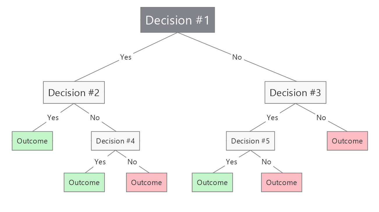
Decision Trees: A decision tree is a predictive model used to determine the outcome based on a set of input features⁹.Its structure is made up of decision nodes, branches, and leaf nodes, where each leaf node represents a prediction for a specific class label. At each level of the tree, an input attribute is chosen as the decision node to split the data into branches based on the attribute’s possible values. The selection of the attribute is guided by a criterion that maximizes classification accuracy, typically by minimizing tree entropy—defined as the amount of information needed to correctly classify the inputs.

(4)  

where represents the entropy, is the number of positive class instances, and is the number of negative class instances. Lower values of indicate that the tree is more effective at distinguishing between the classes.

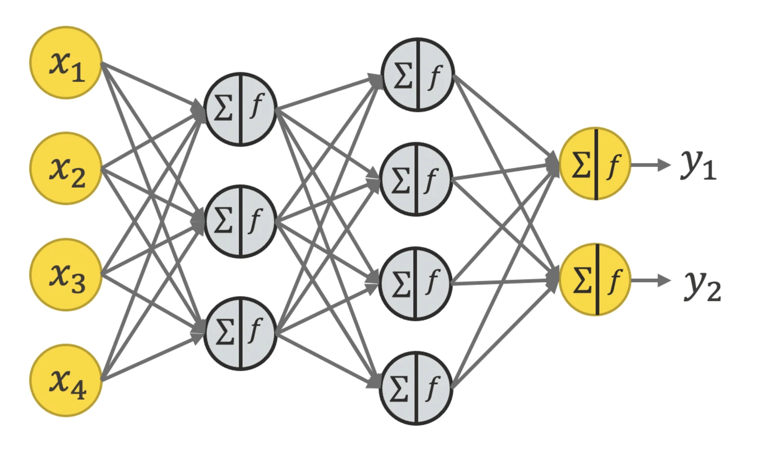
Neural Network: This model is trained to replicate human thought and behavior in data processing¹¹. Neural Networks are computational models made up of layers of interconnected nodes/neurons, with each connection assigned a weight. These networks apply both linear transformations (using weighted connections) and non-linear transformations (using activation functions) to process inputs to generate outputs. The output layer provides predictions or results depending on the task for which the network was trained. Training a Neural Network involves feeding inputs through the network, generating predictions, and comparing them to the true class labels. Any errors are captured and propagated backward through the network using the backpropagation algorithm, which adjusts the weights of the neurons to minimize the error.

The weight update rule during backpropagation is expressed as:

(5)  

where is the weight connecting neuron to , is the error being back propagated, is the learning rate, is the input to neuron , and is the output of neuron . This process is repeated until the network converges on a set of weights that optimize its performance for the given task.

Methodology

Text Preprocessing

Before feeding the text data into logistic regression and XGBoost, we must first preprocess it into a cleaner format. While BERT can process raw text without extensive preprocessing, the other models require additional preprocessing to perform effectively. This is a crucial initial step in NLP tasks, ensuring that the input data retains only the most relevant features for prediction while eliminating unnecessary elements. While the resulting sentence is less readable for humans, it is a more logical representation for the model to process as input. We achieve this by applying the following preprocessing techniques:

1. Remove punctuation
2. Remove numbers
3. Lowercase
4. Remove stopwords (common English words, e.g. “a”, “the”, etc.)
5. Stemming (i.e. retaining only the root of a given word, e.g. “giving” becomes “giv”. This helps to convert different variations of the same word to one representation)

To demonstrate each of these steps, consider the following example:

1. “saw ‘9 to 5’ again and SJB was back! w00000t!!!!! XD She was BRILLIANT as usual; ) and uber sweet at SD  Stephanie J. Block = phenomenal!” (original sentence)
2. “saw 9 to 5 again and SJB was back w00000t XD She was BRILLIANT as usual  and uber sweet at SD  Stephanie J Block  phenomenal” (after removing punctuation)
3. “saw to again and SJB was back w00000t XD She was BRILLIANT as usual  and uber sweet at SD  Stephanie J Block  phenomenal” (after removing numbers)
4. “saw to again and sjb was back w00000t xd she was brilliant as usual  and uber sweet at sd  stephanie j block  phenomenal” (after lowercasing)
5. “saw sjb back w00000t xd brilliant usual uber sweet sd stephanie j block phenomenal” (after removing stopwords)
6. “saw sjb back w00000t xd brilliant usual uber sweet sd stephani j block phenomen” (after stemming)

Classification Models

Technical Specifications

We train our models using the Google Colab environment. By default, Colab gives the user 12.7 GB of RAM. To train DistilBERT, we leverage a T4 GPU which is available in Colab. There is no cost of running any of our models, as we are using the free version of Colab. It takes about an hour to train the DistilBERT model, and just several minutes for Logistic Regression and XGBoost. Each model is efficient and has low inference latency – for example, DistilBERT can run inference on about 760 articles per minute (though of course its model object takes up a significant amount of memory compared to the two simpler models).

Pipeline 1: CountVectorizer + Logistic Regression

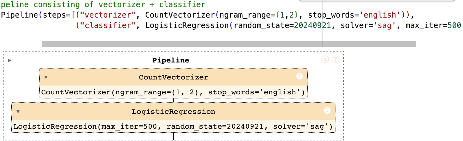
We leverage the scikit – learn package to develop our logistic regression model¹³.Our pipeline consists of a CountVectorizer (which converts the input text into numbers based on word frequency across the entire dataset) and the LR classifier. For CountVectorizer, we set the value of ngram_range to (1,2) (meaning that the model will consider unigrams and bigrams as features), and use the list of English stopwords provided by sklearn. For LR, we set the value of C to 1 (this controls the level of regularization to ensure that the model does not overfit) and the maximum number of iterations to 500; we also use the ‘sag’ solver for fitting the model and a random_state of 20240921 to ensure reproducibility.

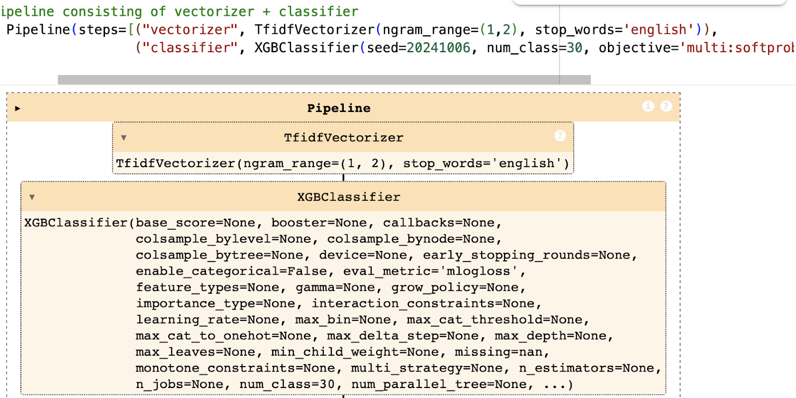
Pipeline 2: TfidfVectorizer + XGBoost

We utilize the XGBoost package to develop our decision tree-based model¹⁴. XGBoost (eXtreme Gradient Boosting) is an ensemble technique consisting of multiple trees, in which each tree is assigned a penalty based on its error frequency so that the next tree can correct those mistakes (hence the term “boosting”). Our pipeline consists of a TfidfVectorizer (which is an extension of CountVectorizer based on term frequency in addition to inverse document frequency) and the XGBClassifier. For TfidfVectorizer, as for CountVectorizer in the previous pipeline, we set the value of ngram_range to (1,2), and use the list of English stopwords provided by sklearn. For XGBClassifier, we set the objective and the evaluation metric to values corresponding to the multiclass classification task (given that we have 30 total classes, compared to the 2 in binary classification) and use a random_state of 20241006 to ensure reproducibility.

Pipeline 3: BERT

For our Neural Network-based model, we select BERT. This transformer model is widely used in NLP. It is pre-trained on large text corpora, including the Google corpus and Wikipedia. This enables it to understand various grammatical structures in English. Fine-tuning BERT on a specific dataset allows it to adapt to domain-specific language, in this case, news media. It still leverages its existing linguistic knowledge. Since BERT already understands raw English text, we do not need to preprocess or vectorize the input data. This step was required for logistic regression and XGBoost.

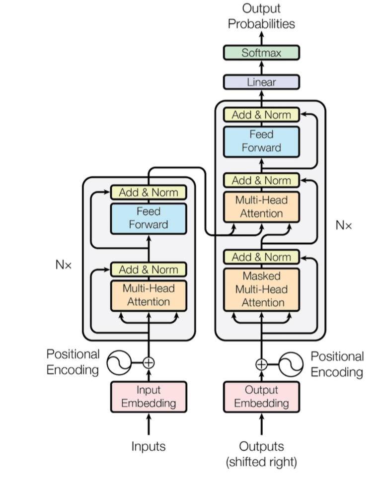
The transformer architecture was first introduced in the paper “Attention Is All You Need,” which proposed a novel NLP framework consisting of an encoder and a decoder, both built as Neural Networks³.BERT operates as an encoder-only model, transforming raw text into a hidden representation and offering multiple variations suited for different tasks. To optimize performance while reducing training time, we use a variant of BERT called DistilBERT¹⁵ . DistilBERT is trained using knowledge distillation, a process that extracts key information from BERT and compresses it into a more efficient architecture while maintaining most of its accuracy. For implementation, we use the base DistilBERT model from Hugging Face, the leading repository for pre-trained NLP models.

The BERT model takes as input a sequence of words comprising a sentence, where each word is represented by a 768-dimensional vector. To retain word order information, we apply positional encoding. This helps the model understand the structure of the sentence. BERT’s transformer-based architecture incorporates a self-attention mechanism. This mechanism determines the significance of words in a given context. For example, in the sentence “A cat jumped over the fence,” key words such as “cat,” “jumped,” and “fence” carry the most meaning for understanding the sentence.  

Once self-attention is applied, BERT performs multi-head attention, followed by a residual connection that bypasses hidden layers by adding the input data directly to the output layer. This approach helps mitigate the vanishing gradient problem, which occurs when gradients become too small during stochastic gradient descent, preventing the model from converging effectively. The processed data is then passed through a feedforward layer, where it is flattened and prepared for classification. Finally, the output layer applies the softmax function to categorize whether a given sentence exhibits bias or toxicity.

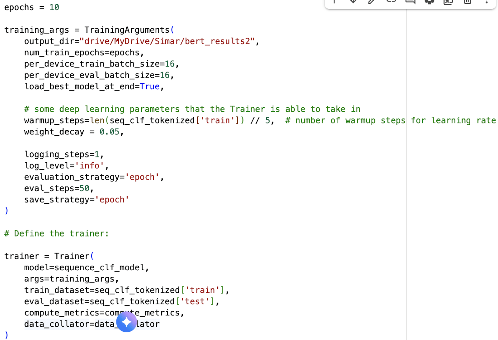
In terms of hyperparameters, we set the number of warmup steps for learning rate equal to 10,898 (20% of the size of our training set), weight decay to 0.05, and batch size of 16. We train the model for 10 epochs.

SHAP Method for Model Interpretability

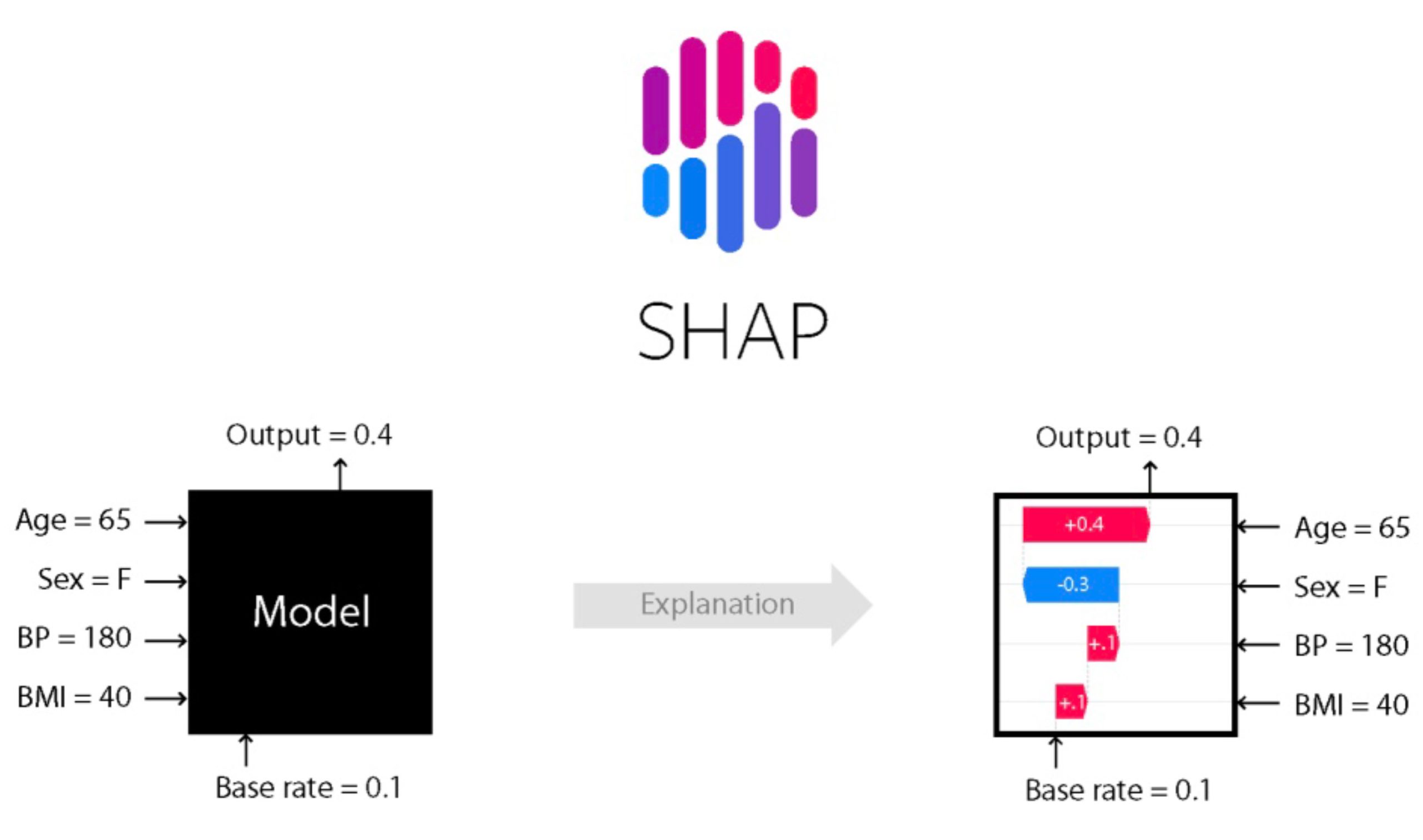
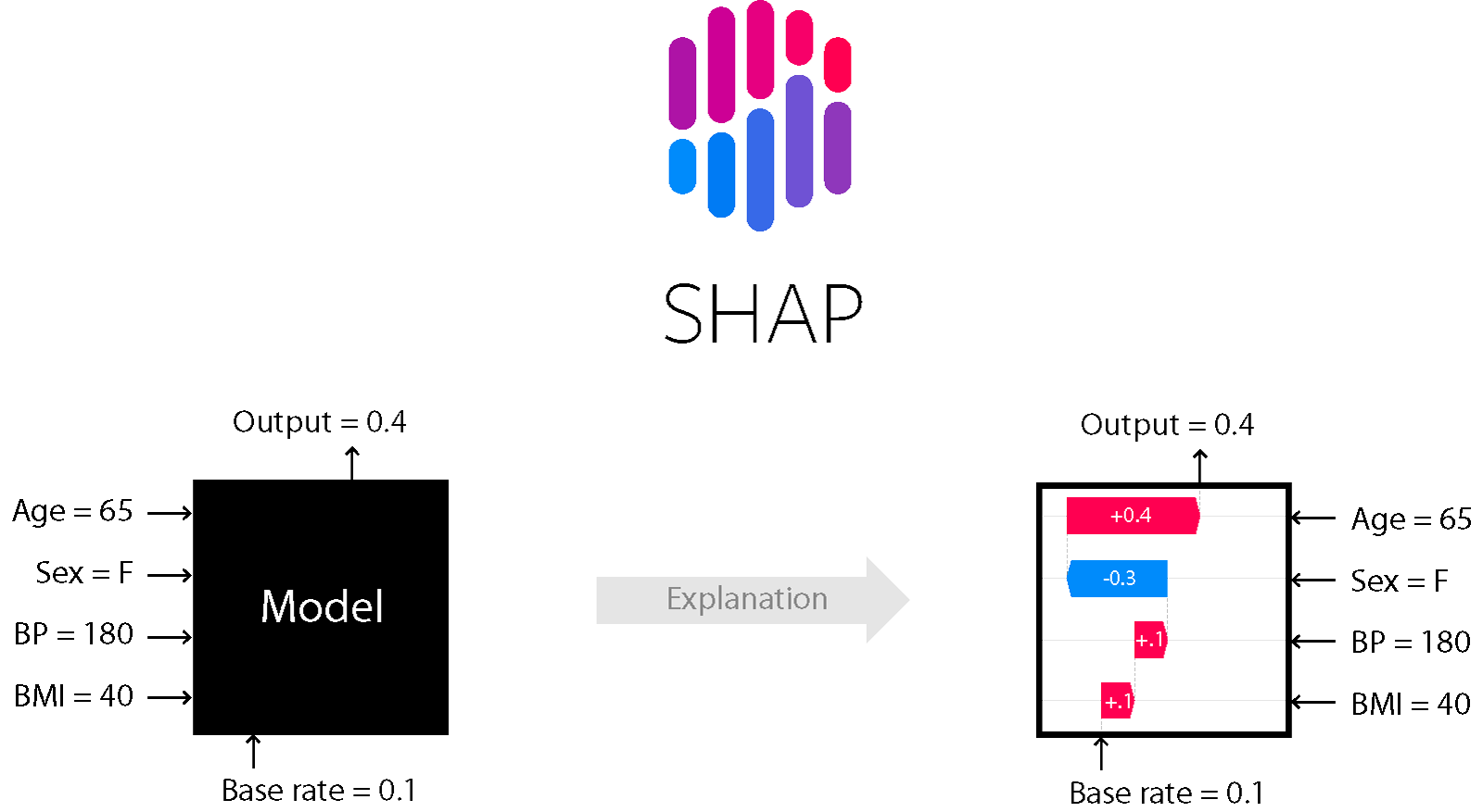
To assess the explainability of our models (namely, XGBoost and BERT), we utilize SHAP (SHapley Additive exPlanations)¹⁶.This package offers tools for interpreting a wide range of machine learning models. SHAP operates as an additive feature attribution method, computing values that quantify how changes in an input feature affect the model’s output. This enables us to determine the significance of specific features in predicting each class, particularly in identifying key n-grams associated with different types and levels of bias. Additionally, SHAP provides various visualization tools that illustrate the relative influence of different n-grams across our three models, enhancing interpretability.

Results

For evaluation, we leverage the existing data which has already been split into training and testing sets by the curators of the dataset. Within each split, we extract all the news articles corresponding to the 5 bias types of interest: confirmation, political, health-related, framing, and gender discrimination. Combined with the three levels of bias (neutral, slight, and high) and the binary label for toxicity, we have a total of 30 possible classes. For the training set, this encompasses 871,876 news articles, while the test set contains 12,129 news articles.

The macro-F1 score for each model reflects its overall performance on the test set. For Logistic Regression, XGBoost, and BERT, these scores are 11.4%, 15.5%, and 47.9%, respectively. As a noteworthy aside, Logistic Regression is the only model which we train on all of the 871,876 available news articles; for the latter two models, we only train on 54,491 articles (i.e. 1/16th of the training set) due to computational resource constraints of our Python environment. Taking this into account, we see that BERT performs significantly better than Logistic Regression (despite being trained on a fraction of the data), and also better than XGBoost on the same amount of data.

To expand on how we select the training set for XGBoost and BERT, we randomly sample 1/16th of the original training set (which amounts to 54,491 articles) using a random_state of 42 for reproducibility. We choose 1/16th because it is not possible to train on any larger fraction of the data, as the Colab notebook tends to run out of memory at a certain point in the training process. We can explore other sampling strategies (e.g. by source) in the future.

The Stanford CS224N project on bias detection in news articles¹⁸ provides a useful point of reference. Their baseline neural models using bag-of-words and TF-IDF features achieved low accuracies of about 15%, while an unsupervised k-means approach failed to separate articles meaningfully. Their strongest model, a SimCSE sentence embedding classifier, reached roughly 24% accuracy. By contrast, in this study, logistic regression and XGBoost performed somewhat better, while BERT substantially outperformed these baselines. This suggests that transformer-based architectures not only surpass simple frequency-based or clustering methods but also scale more effectively to the complexity of a 30-class bias and toxicity framework.

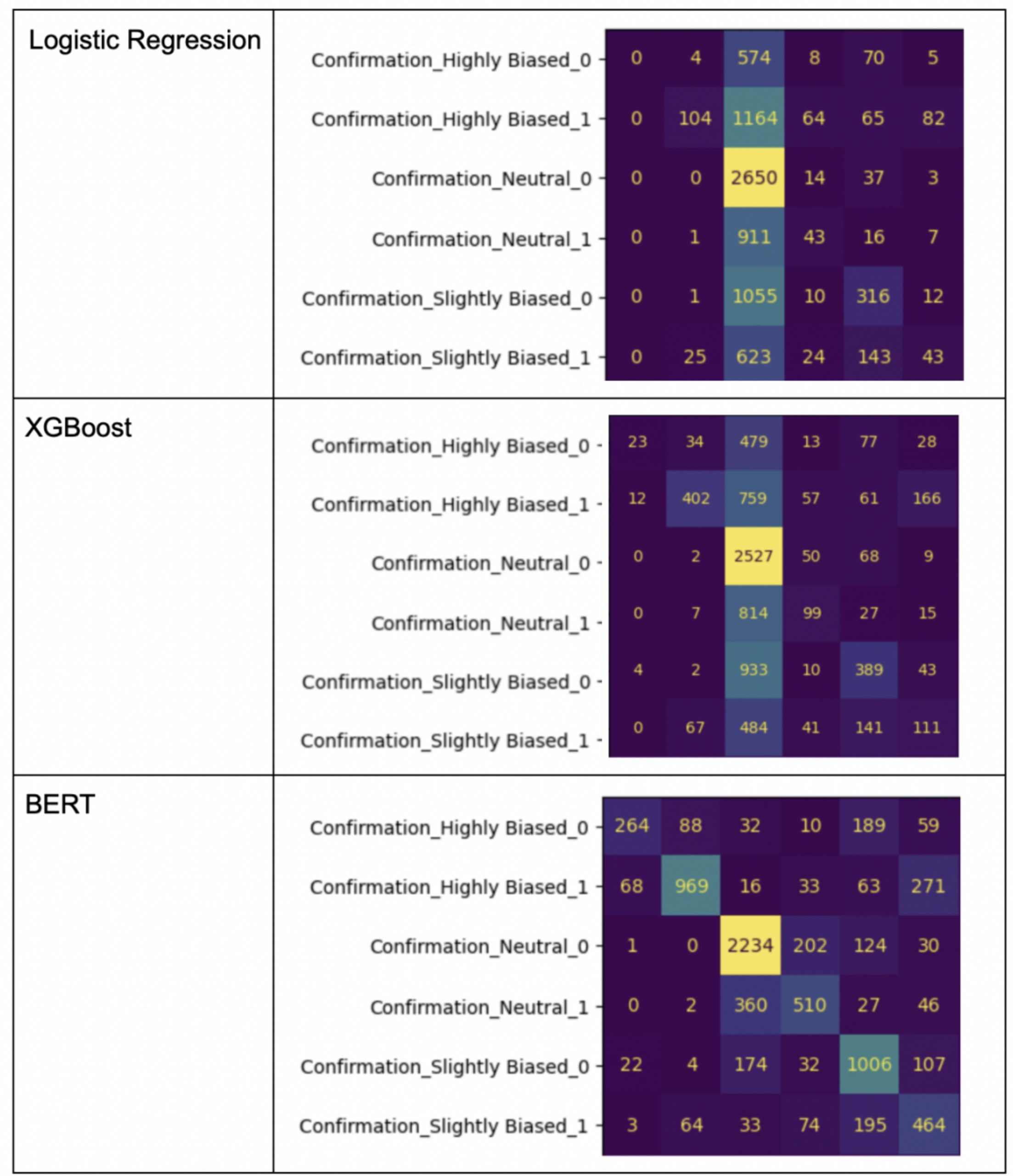
The confusion matrix, displayed below, is a reliable method to assess each model’s performance. This figure compares the number of instances where the predicted label matches the actual label for each of the 30 classes. Intuitively, the larger the numbers on the diagonal of the confusion matrix, the better the performance of the model. While the entire matrix for all 30 classes is too large to include here, we focus on the 6 variants of confirmation bias as an illustrative example. The neutral, not toxic confirmation bias class is the most common in the test set, representing 2,717 instances out of 12,129. Thus, a poorly performing model would attempt to categorize most news articles into this class simply due to its frequency. When we compare the confusion matrices for the three models, we see that Logistic Regression tends to follow this pattern, classifying 2,650 articles as neutral, not toxic confirmation bias. XGBoost performs slightly better with 2,527 such articles, and BERT shows the best performance 

as indicated by the more even distribution of numbers on its confusion matrix.

We can also look at performance of each model per class on the test set, focusing on separate metrics such as precision and recall. Here are the results for the highly biased variants of each bias type, as well as the neutral, non-toxic confirmation bias which is the most common:

		LR			XGBoost			BERT
Class	# of instances	P (%)	R (%)	F1 (%)	P (%)	R (%)	F1 (%)	P (%)	R (%)	F1 (%)
Confirmation, Neutral, Non-Toxic	2,717	29.4	97.5	45.2	33.7	93.0	49.4	74.7	82.2	78.3
Confirmation, Highly Biased, Non-Toxic	678	0	0	0	59.0	3.4	6.4	69.5	38.9	49.9
Confirmation, Highly Biased, Toxic	1,515	50.0	6.9	12.1	62.7	26.5	37.3	79.8	64.0	71.0
Framing, Highly Biased, Non-Toxic	62	0	0	0	100	1.6	3.2	51.5	27.4	35.8
Framing, Highly Biased, Toxic	158	0	0	0	75.0	5.7	10.6	71.3	55.1	62.1
Gender discrimination, Highly Biased, Non-Toxic	31	61.5	25.8	36.4	100	3.2	6.3	60.0	67.7	63.6
Gender discrimination, Highly Biased, Toxic	38	0	0	0	0	0	0	48.1	34.2	40.0
Health-related, Highly Biased, Non-Toxic	201	42.9	1.5	2.9	36.4	4.0	7.2	63.6	38.3	47.8
Health-related, Highly Biased, Toxic	527	62.4	15.7	25.2	67.4	27.5	39.1	72.7	67.4	70.0
Political, Highly Biased, Non-Toxic	22	0	0	0	0	0	0	50.0	13.6	21.4
Political, Highly Biased, Toxic	46	20.4	21.7	21.1	10.0	2.2	3.6	59.5	47.8	53.0

As we can see, BERT achieves the highest F1 score across all of these classes. XGBoost occasionally outperforms BERT in terms of precision or recall, while Logistic Regression tends to do worse overall.

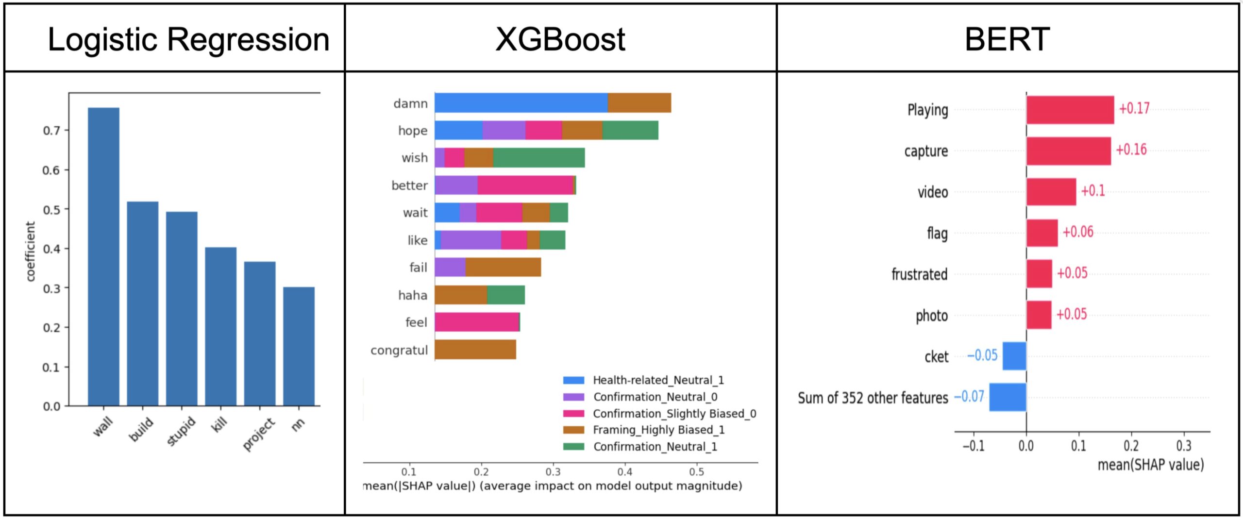
While the confusion matrix serves as a quantitative method to evaluate model performance, the keywords that each model identifies can provide qualitative insight into how well it can distinguish between various bias types. The plots below depict the top keywords that each model captured as being related to framing bias and its highly biased, toxic variant (as well as some other classes in the case of XGBoost). Note that for Logistic Regression, we can directly look at the coefficient associated with each keyword (as the model computes these on its own), whereas for the other two models, we must rely on the SHAP method as an additional tool to obtain the relative scores (Shapley values) for the different keywords. We see that Logistic Regression and XGBoost identify fairly simple words (“wall”, “stupid”, “fail”) that would likely be relevant to multiple kinds of bias, whereas BERT is able to pick up on some words that seem somewhat more specific to framing, at least in certain contexts (“capture”, “frustrated”). BERT may also be identifying words that are not related to framing bias, but perhaps framing in a different sense of the word (“video”, “photo”). This outcome showcases BERT’s knowledge of various linguistic phenomena and its ability to segment concepts based on their meaning, which more traditional models like the former two cannot do quite as well. While SHAP analysis offers valuable insight into model decision-making, some highlighted terms do not clearly relate to the bias being evaluated. For example, BERT occasionally assigns importance to words like “flag” or “playing” under framing bias. We treat these cases as noise in the feature attribution process and emphasize that interpretability requires distinguishing between truly bias-relevant terms and spurious signals. To address this, we focus our discussion on the keywords that consistently align with intuitive class distinctions, while recognizing that not all SHAP outputs are equally informative.

Discussion

Evaluation of Hypothesis

Conducting a qualitative assessment of the results in relation to the hypothesis, we see that the overall connotation of the words identified by our models aligns with that of the most common words found throughout the various news articles. In particular, we can observe that as the complexity of the model increases, it can more effectively pick up on more advanced degrees of bias. For example, referring back to framing bias, Logistic Regression (our most basic model) is able to identify the word “stupid”, which we noted as being associated with a slightly biased, toxic variant. XGBoost, meanwhile, picks up on the word “fail”, which can be used in similar contexts as the phrase “mad wrong” corresponding to the highly biased, toxic variant of framing. Our most sophisticated model, BERT, can identify words for both non-toxic and toxic variants of highly biased framing (“capture”, which is similar to “blocks entirety”, and “frustrated”, which is fairly close to “mad” in the phrase “mad wrong”). Thus, the more advanced model does a better job of capturing higher levels of bias and different options for toxicity, which makes intuitive sense given that it was exposed to a greater variety of language during pre-training. This result likely holds for the other types of bias included in the dataset as well.

In general, our experiments show that out of the models we tested, BERT is the best at picking up on bias-related language. The keyword analysis that we perform in this work can enhance the interpretability of the model, which is particularly crucial to end users who may wish to understand the decision-making process used to assign a certain type and level of bias to a given news article.

Qualitative Assessment on Monkeypox Dataset

The following analysis aims to examine the types of language that can unintentionally influence readers. Journalists can use these insights to strike a balance between delivering important health information and maintaining neutrality, ensuring that their reporting remains objective and trustworthy.

The dataset consists of monkeypox-related articles that were broken down and analyzed to detect various forms of bias, with the goal of helping journalists distinguish between biased and unbiased language. We had 117 articles in total that were predicted into different classes. Applying our models to these articles, the distribution of select predicted classes is as follows:

Health-related, Neutral, Non-Toxic	43
Health-related, Slightly Biased, Non-Toxic	24
Confirmation, Neutral, Non-Toxic	12
Gender discrimination, Slightly Biased, Toxic	2
Health-related, Highly Biased, Toxic	1

For each sentence, the model returned a probability for the associated predicted class. Here are a few examples of the sentences and their outputs:

Morocco has confirmed a case of mpox in a man in the city of Marrakech, the health ministry said	Health-related, Neutral, Non-Toxic
The virus, previously known as monkeypox, can spread through contact with infected animals or people, or through the consumption of contaminated meat	Health-related, Highly Biased, Toxic
Mpox can be spread through close person contact with someone who is infected	Health-related, Slightly Biased, Toxic
“In the Democratic Republic of Congo, their access to the impact vaccine is limited,” he said	Political, Slightly Biased, Non-Toxic
Previously the outbreak had been concentrated in the Democratic Republic of Congo	Political, Neutral, Non-Toxic

For example, the sentence “Mpox can be spread through close person contact with someone who is infected” was labeled as Health-related Slightly Biased with a predicted probability of 0.544. In contrast, “Morocco has confirmed a case of mpox in a man in the city of Marrakech, the health ministry said” was classified as Health-related Neutral with a much higher predicted probability of 0.920. The model tends to label statements containing guidance or warnings as slightly biased, as they may reflect interpretative or persuasive language, whereas factual, objective reporting is more likely to be labeled as neutral.

Additionally, the sentence ” “In the Democratic Republic of Congo, their access to the impact vaccine is limited,” he said” was labeled as Political Slightly Biased with a predicted probability of 0.643. This was most likely labeled as slightly biased because this could unintentionally suggest that the country itself is the problem rather than acknowledging external factors. In contrast, more factual statements, such as “Previously the outbreak had been concentrated in the Democratic Republic of Congo”, was classified as Political Neutral with a 0.512 probability.

Although the Mpox case study highlights important trends in how bias and toxicity appear in reporting on emerging health crises, the dataset is very limited in size, with only 117 articles. Such a small sample restricts the ability to generalize findings and raises the likelihood that some observed patterns are specific to this dataset rather than broadly representative. For this reason, the Mpox analysis should be read as exploratory, offering preliminary insights into how the models handle a niche but significant topic, rather than as a definitive conclusion.

In summary, by applying these insights, journalists can better balance the delivery of important health information while maintaining neutrality, making sure that their reporting remains objective and unbiased.

Error Analysis

While the BERT model showcases the best performance of the three models that we tested, it still has some room for improvement in terms of categorizing articles more accurately. For example, looking at the confusion matrix for BERT in Figure 8, we see that 969 articles containing highly biased, toxic confirmation bias are predicted correctly. However, there is a substantial number of articles that BERT placed into other categories, such as 16 that are predicted as neutral and non-toxic and 271 predicted as slightly instead of highly biased. These numbers illustrate the mistakes that BERT can make in distinguishing between levels of bias and toxicity, which can potentially be improved with further fine tuning.

Another indicator of BERT’s flaws in bias comprehension is the SHAP analysis used to identify the top keywords for each bias type. Looking at the list of keywords that BERT associated with framing bias in Figure 9, we see that some of them (e.g. “playing”, “flag”) may actually not be relevant in such contexts. A more robust model would be able to filter out keywords that are not truly indicative of the given phenomenon so as to ensure proper interpretability. Again, this can be improved by fine tuning BERT in a more extensive manner.

Due to computational constraints, the BERT model was trained on only a subset of the dataset, making direct comparisons with models trained on the full dataset less balanced; future work should employ approaches such as distributed training or cloud GPUs to ensure more equitable evaluations.

To further mitigate the effects of dataset imbalance, particularly the overrepresentation of categories like confirmation bias and underrepresentation of smaller classes such as gender discrimination, future work should explore balancing strategies such as re-sampling, class weighted loss functions, or other augmentation methods to ensure fairer model performance across all bias categories.

One limitation of this study lies in the Mpox case subset, which contains only 117 articles. The small dataset size makes model performance more sensitive to noise and less reliable for drawing firm conclusions. While the analysis provides useful early observations, the limited sample reinforces that these results should be treated as exploratory and interpreted with caution.

Real-time bias detection could be valuable, but it also comes with challenges. Running large models at scale is costly, fairness across categories must be protected, and media outlets may be hesitant to adopt automated tools. Acknowledging these limits shows that real-time use is possible but not without obstacles.

Automated bias detection carries important risks. False positives could unfairly label articles, creating stigma or discouraging certain types of reporting. Models can also amplify existing dataset biases, which may skew results further. To limit these harms, systems should include human oversight, set confidence thresholds before flagging content, and remain transparent about how decisions are made. These safeguards help balance the promise of automation with the responsibility to protect journalistic integrity.

Looking at the per-class results, the models often misclassify smaller categories such as gender discrimination and political bias, where logistic regression and XGBoost frequently collapse predictions into majority classes. BERT performs better overall, but still struggles with categories that share overlapping language, such as distinguishing between confirmation and framing bias. The confusion is most pronounced for highly biased but non-toxic classes, suggesting that the models pick up toxicity cues more easily than subtle distinctions in tone or framing.

Future Work

Integrating bias and toxicity detection systems into social media and news media platforms can provide real-time indicators of article reliability. Additionally, the development of automated misinformation tracking tools could help policymakers, journalists, and researchers monitor trends in media bias and disinformation campaigns over time. These tools could play a critical role in combating bias within media, particularly in sensitive topics such as elections, public health, and international conflicts. At present, the models are not accurate enough for real-world use, as the F1 scores show they make errors more than half the time. However, the error analysis points to clear areas for improvement, such as class imbalance and limited training data for BERT. Addressing these issues could raise performance to a level where real-world applications become more realistic.

Future work could expand the SHAP analysis to look beyond individual examples. Comparing keyword patterns across different classes and analyzing SHAP value distributions would help identify consistent signals the models rely on, as well as points where they misattribute importance. This broader view would make the interpretability claims more robust and show how different types of bias are reflected in model explanations.

Additionally, a key focus should be on improving misinformation detection techniques related to Mpox and other public health crises. Future models could incorporate fact-checking sources and authoritative medical research databases to assess the credibility of health-related claims in news articles. Analyzing social media discourse alongside traditional news articles could also provide a more comprehensive picture of how misinformation proliferates in different online communities. In addition, we can bring in domain experts who can ensure that the labeling guidelines are consistent with the proper definition of each bias type, as well as conduct an additional qualitative assessment of the models’ performance.

Understanding the sociopolitical framing¹⁹ of Mpox remains an important area of research. The disease has been subject to stigmatizing narratives in certain media reports, particularly regarding certain communities. Future work should investigate how bias intersects with public health journalism, ensuring that reporting on Mpox and similar diseases promotes factual accuracy without reinforcing harmful stereotypes. Developing models that can detect both scientific misinformation and social bias in health reporting would significantly contribute to improving news media literacy and public trust in broadcasting health information.

The Mpox-related media bias analysis presents unique challenges that lead to further investigation. One critical step is expanding the dataset to include a wider range of health-related misinformation, particularly in the context of infectious disease outbreaks, vaccine hesitancy, and public health policy responses. Given the rise of misinformation²⁰ during global health crises, future iterations of this dataset should include a time-series analysis of media framing during different phases of the Mpox outbreak. This could provide insights into how narratives evolved over time²¹ and how misinformation spread across various platforms²².  

By expanding the dataset and integrating real-world applications, this project has the potential to contribute to the global effort to combat misinformation²³ and disinformation²⁴ in news media. The Mpox-related bias analysis provides a valuable case study for understanding how health misinformation spreads²⁵ and how media framing influences public perception of diseases²⁶. Addressing these challenges in future research will help develop more effective bias detection systems ensuring that information is presented fairly, accurately, and responsibly.

Acknowledgments

This research was conducted in Bakersfield, California from June to December 2024.

References

1. Mogotsi, I. C., Manning, C. D., Raghavan, P., & Schütze, H. (2010). Introduction to information retrieval. Information Retrieval, 13, 192–195. https://doi.org/10.1007/s10791-009-9115-y. [↩]
2. Rodríguez-Pérez, R., & Bajorath, J. (2020). Interpretation of machine learning models using Shapley values: Application to compound potency and multi-target activity predictions. Journal of Computer-Aided Molecular Design, 34, 1013–1026. https://doi.org/10.1007/s10822-020-00314-0. [↩]
3. Vaswani, A., Shazeer, N., Parmar, N., Uszkoreit, J., Jones, L., Gomez, A. N., Kaiser, L., & Polosukhin, I. (2017). Attention is all you need. Advances in Neural Information Processing Systems, 30. https://arxiv.org/abs/1706.03762. [↩] [↩]
4. Raza, S. (2023). Navigating news narratives: A media bias analysis dataset. arXiv preprint arXiv:2312.00168. https://arxiv.org/abs/2312.00168. [↩]
5. Mogotsi, I. C., Manning, C. D., Raghavan, P., & Schütze, H. (2010). Introduction to information retrieval. Information Retrieval, 13, 192–195. https://doi.org/10.1007/s10791-009-9115-y [↩]
6. Optiz, J. (2022). From bias and prevalence to macro F1, kappa, and MCC: A structured overview of metrics for multi-class evaluation. Heidelberg University. [↩]
7. Ji, Z., & Telgarsky, M. (2019). The implicit bias of gradient descent on nonseparable data. In Conference on Learning Theory (pp. 1772–1798). PMLR. [↩]
8. Zaidi, A., & Al Luhayb, A. S. M. (2023). Two statistical approaches to justify the use of the logistic function in binary logistic regression. Mathematical Problems in Engineering, 2023, 5525675. https://doi.org/10.1155/2023/5525675. [↩]
9. Quinlan, J. R. (1986). Induction of decision trees. Machine Learning, 1(1), 81–106. https://doi.org/10.1007/BF00116251. [↩]
10. MindManager. (n.d.). Decision tree diagram. Retrieved September 10, 2025, from https://blog.mindmanager.com/decision-tree-diagrams/. [↩]
11. Rumelhart, D. E., Hinton, G. E., & Williams, R. J. (1986). Learning internal representations by error propagation. In Parallel distributed processing: Vol. 1 Foundations. MIT Press. [↩]
12. Mondal, S. (2022). Neural Network from scratch. Medium. https://saankhya.medium.com/neural-network-from-scratch-82642047ff84. [↩]
13. Pedregosa, F., Varoquaux, G., Gramfort, A., Michel, V., Thirion, O., Grisel, O., Blondel, M., Prettenhofer, P., Weiss, R., Dubourg, V., Vanderplas, J., Passos, A., Cournapeau, D., Brucher, M., Perrot, M., & Duchesnay, E. (2011). Scikit-learn: Machine learning in Python. Journal of Machine Learning Research, 12, 2825–2830. https://arxiv.org/abs/1201.0490. [↩]
14. Chen, T., & Guestrin, C. (2016). XGBoost: A scalable tree boosting system. In Proceedings of the 22nd ACM SIGKDD International Conference on Knowledge Discovery and Data Mining (pp. 785–794). ACM. https://arxiv.org/abs/1603.02754. [↩]
15. Sanh, V., Debut, L., Chaumond, J., & Wolf, T. (2019). DistilBERT, a distilled version of BERT: Smaller, faster, cheaper and lighter. arXiv preprint arXiv:1910.01108. https://arxiv.org/abs/1910.01108. [↩]
16. Lundberg, S. M., & Lee, S. (2017). A unified approach to interpreting model predictions. Advances in Neural Information Processing Systems, 31. https://proceedings.neurips.cc/paper/2017/hash/8a20a8621978632d76c43dfd28b67767-Abstract.html. [↩]
17. Lundberg, S. M., & Lee, S. (2017). SHAP (SHapley Additive exPlanations). SHAP Documentation. Retrieved September 10, 2025, from https://shap.readthedocs.io/en/latest/_images/shap_header.png. [↩]
18. Stanford CS224N. (2022). Detecting bias in news articles using NLP models [Course project report]. Stanford University. Retrieved from https://web.stanford.edu/class/archive/cs/cs224n/cs224n.1224/reports/custom_116661041.pdf. [↩]
19. Berk, N. (2025). The impact of media framing in complex information environments. Political Communication. Advance online publication. https://doi.org/10.1080/10584609.2025.2456519. [↩]
20. Adams, Z., Osman, M., Bechlivanidis, C., & Meder, B. (2023). (Why) Is misinformation a problem? Perspectives on Psychological Science, 18(6), 1436–1463. https://doi.org/10.1177/17456916221141344. [↩]
21. The Evolution of Digital Storytelling: From Blogs to Vlogs … (2025). International Journal of Research Publication and Reviews, 6(5), [article]. Retrieved from https://ijrpr.com/uploads/V6ISSUE5/IJRPR46461.pdf. [↩]
22. Mathew, S. K., & T. S. Muhammed. (2022). The disaster of misinformation: A review of research in social media. International Journal of Data Science and Analytics, 13(4), 271–285. https://doi.org/10.1007/s41060-022-00311-6. [↩]
23. Lee, J. H., Santero, N., Bhattacharya, A., May, E., & Spiro, E. S. (2022). Community-based strategies for combating misinformation: Learning from a popular culture fandom. Misinformation Review. https://misinforeview.hks.harvard.edu/article/community-based-strategies-for-combating-misinformation-learning-from-a-popular-culture-fandom/. [↩]
24. Shu, K., Sliva, A., Wang, S., Tang, J., & Liu, H. (2020). Combating disinformation in a social media age. Wiley Interdisciplinary Reviews: Data Mining and Knowledge Discovery, 10(6), e1385. https://doi.org/10.1002/widm.1385. [↩]
25. Kbaier, D., Kane, A., McJury, M., & Kenny, I. (2024). Prevalence of health misinformation on social media—Challenges and mitigation before, during, and beyond the COVID-19 pandemic: Scoping literature review. Journal of Medical Internet Research, 26, e38786. https://doi.org/10.2196/38786. [↩]
26. Young, M. E., Norman, G. R., & Humphreys, K. R. (2008). Medicine in the popular press: The influence of the media on perceptions of disease. PLOS ONE, 3(10), e3552. https://doi.org/10.1371/journal.pone.0003552. [↩]