
Abstract
Investment in solar photovoltaics (PV) systems has increased to meet global green energy targets. However, dust accumulation (soiling) on PVs creates a significant reduction in output power and increases cleaning costs. At a global PV capacity above 500 GW, billions of gallons of water are used annually for cleaning purposes. This is problematic for desert areas where water is scarce, especially because the abundance of sunlight in these regions makes them favorable for solar power production. Thus, optimizing PV cleaning schedules is crucial to make solar energy more sustainable. Therefore, this study proposed an algorithm that optimizes weekly cleaning schedules using publicly available environmental forecasts. This involves a feed-forward neural network, a soiling degradation analysis, and a cost-benefit analysis that factors in estimated cleaning costs and value of electricity to find the optimal day to clean. This model was trained on a dataset from an NREL soiling station to forecast daily power output, with its hyperparameters being tuned incrementally to maximize accuracy. The algorithm was tested over a six-year simulation from this dataset using varying cleaning cost estimates. Results showed that the maximum output power increase is 7.9%, with an 82.6% decrease in cleaning events using this algorithm and a relatively stable output power increase across the many cleaning costs. This indicates great potential to improve the economic viability and resource efficiency of PV systems without relying on drastic technological advancements in PV systems.
Keywords: solar; photovoltaics; cleaning schedule; soiling; neural network; output power
Introduction
Currently, increasing demand for energy around the world is met with the more readily available fossil fuels, which pose not only environmental factors and health concerns but are also contributing to climate change1. For these risks, replacement with greener energy is vital. Of renewable energies, solar photovoltaic (PV) systems are generally favored due to their easier accessibility and higher rates of return2. However, the current efficiency of commercial PVs are only around 15% to 23%, thus further advancements are needed to improve their competitiveness3.
The output power of PV systems is affected by several environmental factors including temperature, solar radiation, and dust. The soiling or accumulation of dust on PVs prevents the transmission of light rays to the surface of solar cells4 and can reduce PV output power by 8% to 12% per month5. The degree and rate of soiling varies greatly in different areas around the world, depending on the climate and surrounding environment6. Large-scale solar plants are often located in regions with an abundance of land and sun, such as deserts. However, not only does dust accumulation pose a larger issue in these regions, water for cleaning is also more scarce7. Water based cleaning accounts for up to 10% of maintenance and operation costs, consuming up to 10 billion gallons of water, enough to supply 2 million people with drinking water8. Therefore, unoptimized PV cleaning schedules can even more greatly reduce the feasibility of PV systems as a sustainable and economic source of electricity9,10.
In order to optimize the cleaning of PVs, researchers have developed methods to detect dust. Image processing has been used for dust detection including Gao et al.’s system using moving infrared cameras to detect dust and panel defects (which had an accuracy of 97.9%) and Ramos et al.’s system using cameras on terrain robots (which had an accuracy of 90%)11. Tsamaase et al. combined dust detection and automated cleaning using a simple Arduino based system with a light sensor to determine whether power output was lower than 80% the expected amount and therefore whether it was necessary to clean12. Although systems such as Gao et al. and Ramos et al.’s show promising results, these systems typically require expensive sensors, cameras, and other detection devices. Meanwhile, cheaper options such as Tsamaase et al.’s Arduino based system rely on less precise methods of detection and can be expensive to scale to the size of larger solar plants. Additionally, they detection devices must be maintained and supplied electricity, incurring even greater costs.
For this reason, researchers have attempted to design sensorless dust detection systems. Shaaban et al. trained regression models to use solar irradiance, temperature, and output power to predict dust levels and therefore create a cleaning schedule13. Skomedal and Deceglie have successfully designed an algorithm to predict both the effect of soiling and degradation in solar panels14, and Alfaris has proposed a sensorless intelligent system for dust detection to improve PV cleaning schedules15. Alvarez has also developed a schedule algorithmically based on cleaning costs, annual radiation, and PV module degradation16.All of these previous algorithms were designed to develop regimented cleaning schedules rather than ones that varied in response to active input. They often depended on graphical analysis or equations to determine a fixed number of days between each cleaning.
Therefore, we propose an algorithm that is more adaptable because of how it predicts the optimal cleaning time using AI depending on the environmental conditions and condition of the solar panel each week. The goal is to minimize water consumption, while maintaining, if not increasing the output power production over time. This algorithm uses a feed-forward neural network, a soiling degradation analysis, and a cost-benefit analysis that factors in estimated cleaning costs and value of electricity to find the optimal day to clean. This model is trained on a dataset from an NREL soiling station to forecast daily power output, with its hyperparameters being tuned incrementally to maximize accuracy. The testing involves running this algorithm over a six-year simulation to see how output power production and the number of cleaning events are affected. One limitation is how the feasibility of this algorithm is hard to verify because of lack of data about the cleaning costs associated per cleaning event. Thus, the testing also involves running these simulations again for different scenarios with different cleaning costs.
Methods
The overall structure of this study is experimental and longitudinal, as we develop and test a neural network-based algorithm to determine optimal cleaning schedules for PV systems under varying conditions and then applied over a six-year simulation to evaluate the overall performance and trends. The experimentation was conducted on an Apple Silicon M4 Chip and on a Python virtual environment.
First, the dataset is collected. The first dataset used is publicly available and collected from NREL (National Renewable Energy Lab) soiling station 4. It can also be accessed from the PVDAQ (Photovoltaic Data Acquisition Public Datasets) database. This is time series data from a PV system, PVDAQ system 4 from 2010 – 2016. This plant is located in Fresno, California. The data has values for solar irradiance, wind speed, ambient temperature, and soiling numbers as synthesized by the RdTools Algorithm that is associated with this dataset. Then, it is processed. Outliers are removed by identifying which values don’t fall within the interquartile range of each of the mentioned columns, and then the data is grouped by days. The environmental factors are averaged out, and the ac_power is added across all the days to get the final value in kWh/day. This dataset shall be referred to as dataset 1 from here on.
This process was repeated for two more datasets. These datasets also contained a sizable amount of noise, so outliers had to be removed in a similar manner. There were also several sensors measuring the same environmental feature, such as ambient temperature or POA (plane of array) irradiance, so the readings from these sensors were averaged to get a better reading. The second dataset is also publicly available from PVDAQ. It also contains approximately 6 years of data from 2017 to 2023. This is time series data with 5 minute intervals from a plant located in Kersey, Colorado. This dataset shall be referred to as Dataset 2. The third dataset is also from PVDAQ. It contains 3 years of data from 2020 to 2023 after processing. This is time series data with 5 minute intervals from a plant located in Georgia. This dataset shall be referred to as Dataset 3. These two datasets also have values for solar irradiance, wind speed, and ambient temperature. It does not have data for the soiling number, so RdTools had to be implemented again.
For the initial data analysis, the relationship between the PV output power and the soiling number was plotted, as shown in Figure 4. This figure shows the complex relationship between PV output power and soiling that is clearly affected by other environmental factors. It also indicates that there is a noticeable positive correlation between PV output power and soiling overall. Specifically, the range of PV output power values is smaller for lower soiling numbers and bigger for larger soiling numbers. This effect is far more pronounced for the second and third graphs, where there are less data points, because this RdTools implementation required daily data while the first dataset already had synthesized soiling data at minute intervals.


Next, the PV output power prediction model is trained with temporal cross validation with an expanding window to maintain the chronological order of the data points. The train-validation-test split is 60 : 20 : 20 and the window and step sizes are adjusted according to the size of the datasets. Different models are tested to verify which model/network is best fit for this dataset. In the end, a feed-forward neural network was determined to be the best fit. First, the initial weights/biases need to be set in order to make sure the model doesn’t waste time in the early epochs with extremely high training losses. Second, it’s best practice to overfit the model on one batch. For this step, the model would have very low complexity. This step is to ensure that the model is, at the very least, able to extract information from the data. Now, the next step is to add complexity to the model one at a time. The important parameters are the number of layers, number of neurons in each layer, activation functions, regularization techniques, and the number of epochs that the model will be trained on.
Ideally, this model should achieve at least an RMSE less than 10% of the range, because this model is the foundation for the proposed algorithm. The core idea behind this algorithm is to develop the cleaning schedule in pieces by considering cases weekly, then breaking it down to a daily basis. If this algorithm were to be implemented, it would be run every week. The user would be required to input the environmental data forecast for the upcoming week. The data required is solar irradiance, wind speed, and ambient temperature predictions for the next week, which are freely available to the public on the Internet. In this algorithm, the soiling number shall be approximated by estimating a nonlinear degradation rate using the CODS (Combined Estimation of Degradation and Soiling Losses) algorithm and the library RdTools14. It is also assumed that there is no merit in cleaning more than once a week due to the average soiling degradation rate not being large enough to cause a significant change that makes it worthwhile to clean twice within a week. Therefore, there are 7 cases for cleaning, one for each day of the week. In each case, the total output power (Ppred) is predicted using the neural network. Then at the end of this simulation, the case that produces the maximum output power (Pmax) is considered, but this option is not chosen automatically. This is also depicted in the flowchart in Figure 5.
Now, an analysis is done every week to make sure that there is enough increase in output power to warrant a cleaning.
![\[P_{\max} \times val > P_{WC} \times val + C\]](https://nhsjs.com/wp-content/ql-cache/quicklatex.com-f2f1cf18d74438d0c051b8c81d94b82d_l3.png "Rendered by QuickLaTeX.com")
PWC refers to the output power that would have been produced if the panels were not cleaned at all. val refers to the value of electricity in the location of the solar panels. Lastly, C refers to the cost of cleaning, including both the private cost and social cost of the water consumption. In order to make code implementation simpler, the equation is also manipulated into this
![\[P_{\max} > P_{WC} + \frac{C}{val} \implies P_{\max} > P_{WC} + Q\]](https://nhsjs.com/wp-content/ql-cache/quicklatex.com-6ac3c58cc056988cc66535bcdc023740_l3.png "Rendered by QuickLaTeX.com")
This indicates how the Q coefficient has the potential to be applied specifically to different locations and types of PV plants with different values of electricity and cleaning costs. A range of Q coefficients shall be tested to see the correlation between the cleaning cost and the corresponding change in output power and number of cleaning events according to this algorithm. For each Q coefficient, the algorithm shall be run across the temporal range of the dataset according to the flowchart in Figure 5. The code will also stop when it reaches a Q coefficient where the algorithm determined that it was optimal to not clean the solar panels any week because the cost was too high.

Results/Analysis
A. Output Power Prediction Model
The size of the initial dataset only had 2314 samples after the data with one-minute intervals was consolidated into daily samples. The size of the two other datasets also only had 6000 samples after consolidation. To address the limited size, we applied jitter-based augmentation by generating 10 jittered versions of each sample, expanding the dataset to approximately 20,000 samples. We also used a fixed random seed to improve reproducibility.
After extensive testing and experimentation of various layers of the model, a suitable model was created with 5 dense layers, batch normalization, and a HeUniform kernel initializer. It was complied with a mean squared error loss function, an Adam optimizer, a learning rate of 3e-4, and gradient clipping. Then it was trained with temporal cross validation with 200 epochs, a batch size of 64, and early stopping.
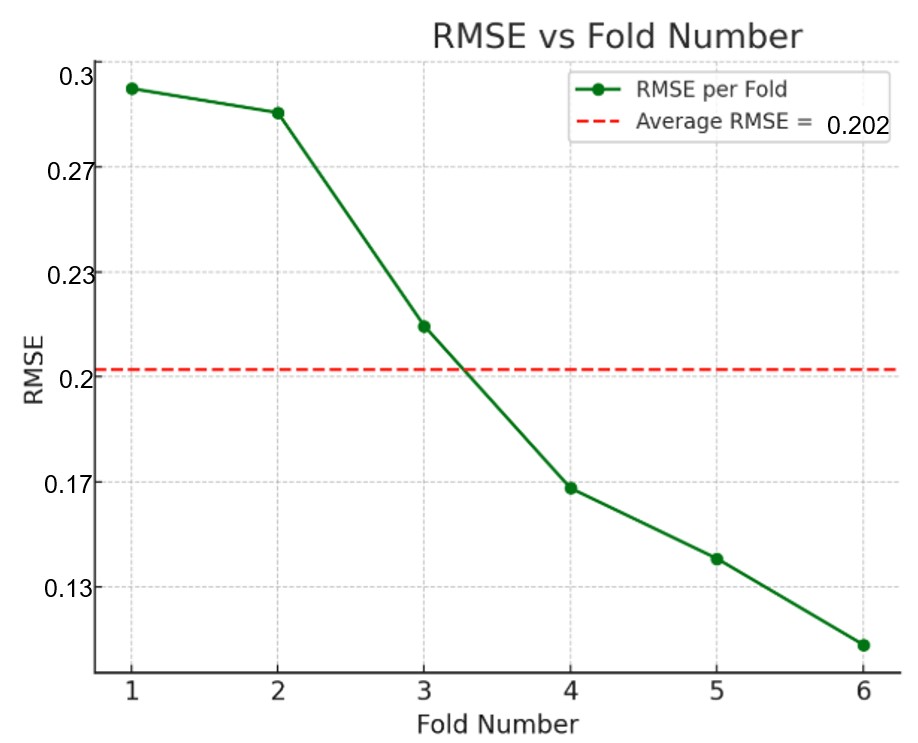
Figure 3a shows the performance of the model at each test fold during the training. The average RMSE across each test fold was 0.20 kWh/day. The average width of the 95% prediction intervals was approximately 0.384 kWh/day, representing about 5.5% of the target variable’s full range (6.97) and roughly 23% of its standard deviation (1.67).
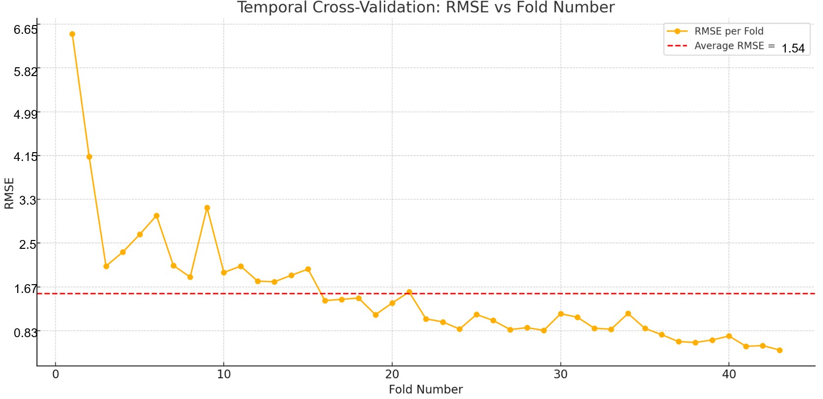
Figure 3b shows the performance of the model when training it on Dataset 2. The average RMSE across each test fold was 1.54 kWh/day. The average width of the 95% prediction intervals was approximately 1.48 kWh/day, representing about 3.4% of the range (43.84) and 13.5% of its standard deviation (10.93).
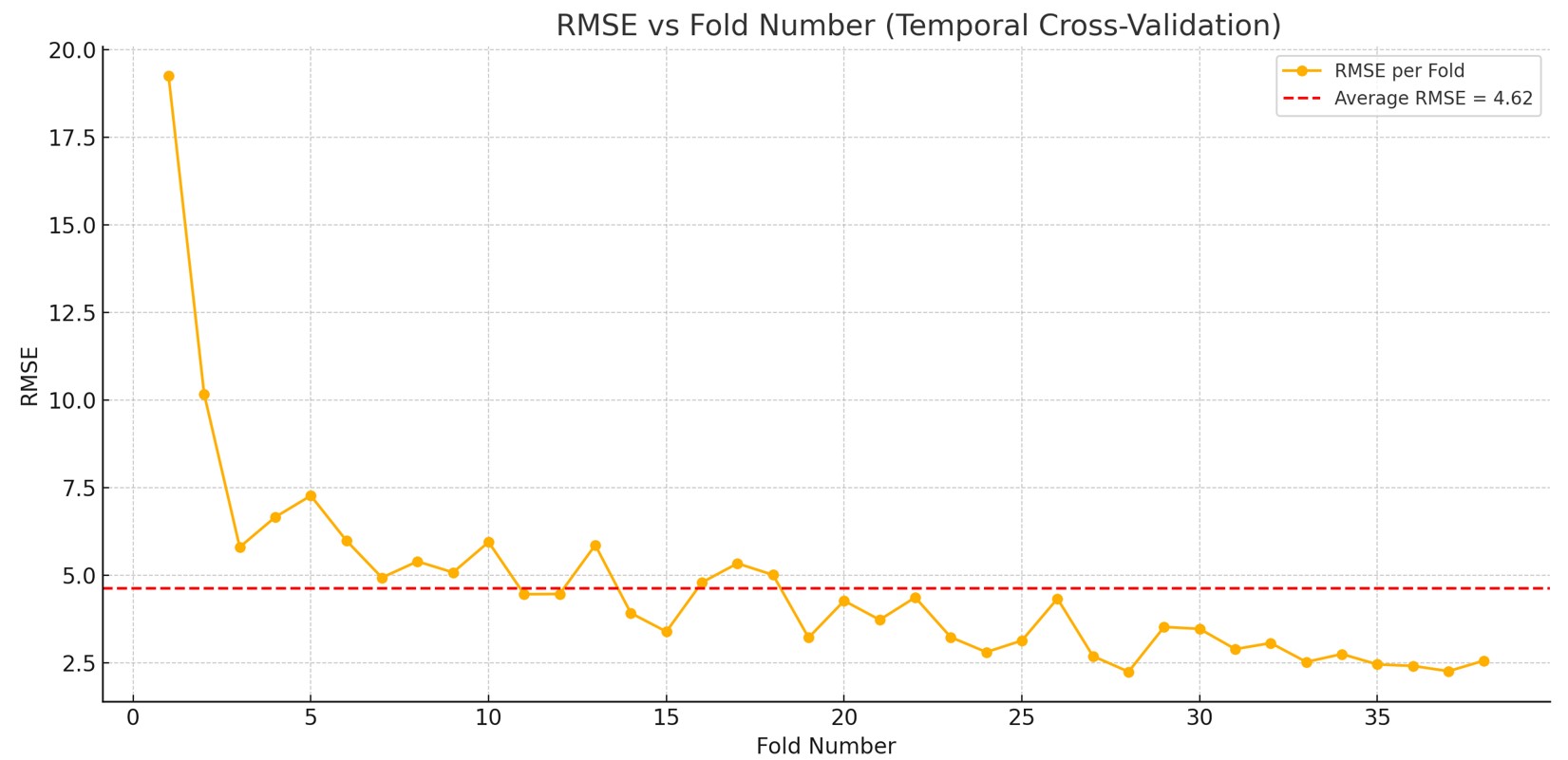
Lastly, Figure 3c shows the performance of the model when training it on Dataset 3. The average RMSE across each test fold was 4.62 kWh/day. The average width of the 95% prediction intervals was approximately 7.41 kWh/day, representing about 3.1% of the range (241.76) and 13.3% of its standard deviation (55.6).
This indicates that the model has excellent accuracy and provides reasonably tight uncertainty bounds around its predictions across the different datasets.
B. Validation of Algorithm
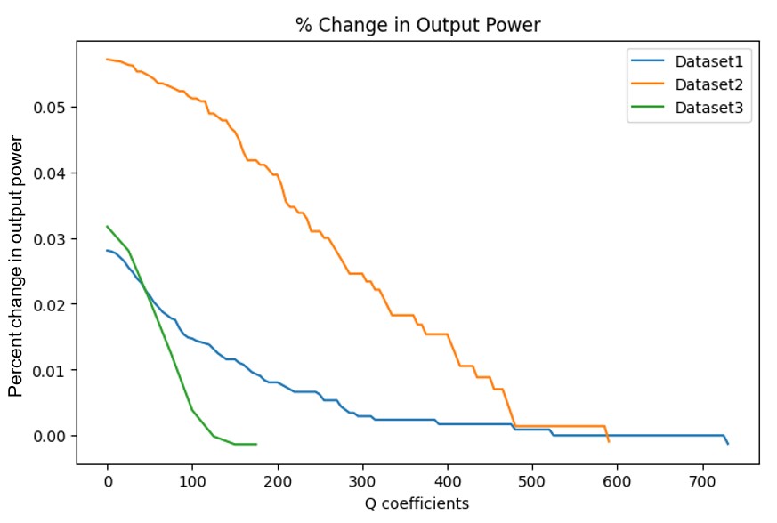
The algorithm is validated by testing its performance across a range of Q coefficients or cleaning costs. The average amount of time it took to simulate the algorithm across the datasets was 5.5 hours. The best results were an increase in output power up to 5.7%.
Overall, Figure 4 shows how there is a clear negative correlation between the percentage increase in output power and the Q coefficients. This was expected because of how Figure 3 shows how greater Q coefficients means greater cleaning costs, which in turn means less cleaning events.
Another noticeable pattern is the clear correlation between the maximum Q coefficient reached for each dataset, before the algorithm concluded that further cleaning was no longer cost-effective, and the size of the solar plant. This supports the idea that the algorithm effectively recognizes when cleaning a smaller plant isn’t worthwhile due to insufficient gains in energy production.

Discussion
The results suggest that water consumption can be significantly reduced without decreasing the output power, even increasing the output power in some cases. Across a lot of different scenarios with different cleaning costs, we have found that the output power production increase in each scenario was relatively the same. This shows that this algorithm is resource-efficient and cost-effective. Furthermore, the Q coefficients can help the user choose what cleaning method would be most cost-effective for them and how often they should clean. It takes a few seconds to run the algorithm each week, meaning the system is relatively low maintenance. In addition, because the inputs can all be found on the internet for free, no additional costs to maintain sensors and other devices is necessary. However, implementations could be simplified for the user by creating a solar irradiance model or having inputs automatically taken from online depending on the user’s resources. Using a neural network or even a model with Long-Short Term Memory layers can help make a better prediction of the soiling numbers while considering previous soiling numbers and current environmental data. In addition, if we had better data on cleaning costs, we could further validate the effectiveness of our algorithm and economic feasibility. This algorithm has the potential to minimize the usage of water while maximizing the output of PV systems, making solar energy more sustainable, especially in arid regions.
Acknowledgements
Thank you to Dr. Movshovitz for mentoring our project. Special thanks to Michael Deceglie for clarifying the details of the dataset used in this study.
References
- S. Shahriar, E. Topal. When will fossil fuel reserves be diminished? Energy Policy. 37, 181-189 (2009). [↩]
- K. Nadarajah, D. Vakeesan. Solar energy for future world: – A review. Renewable and Sustainable Energy Reviews. 62, 1092-1105 (2016). [↩]
- M.S. Ismail, M. Moghavvemi, T.M.I. Mahlia. Characterization of PV panel and global optimization of its model parameters using genetic algorithm. Energy Conversion and Management. 73, 10-25 (2013). [↩]
- A. H. Alami, M. K. H. Rabaia, E. T. Sayed, M. Ramadan, M. A. Abdelkareem, S. Alasad, A. Olabil. Management of potential challenges of PV technology proliferation. Sustainable Energy Technologies and Assessments. 51, 101942 (2022). [↩]
- H. Salimi, A. M. Lavasani, H. Ahmadi-Danesh-Ashtiani, R. Fazaeli. Effect of dust concentration, wind speed, and relative humidity on the performance of photovoltaic panels in Tehran. Energy Sources, Part A: Recovery, Utilization, and Environmental Effects. 45, 7867–7877 (2019). [↩]
- S. You, Y. J. Lim, Y. Dai, C. Wang. On the temporal modelling of solar photovoltaic soiling: Energy and economic impacts in seven cities. Applied Energy. 228, 1136-1146 (2018). [↩]
- K. K. Ilse, B. W. Figgis, V. Naumann, C. Hagendorf, J. Bagdahn. Fundamentals of soiling processes on photovoltaic modules. Renewable and Sustainable Energy Reviews. 98, 239-254 (2018). [↩]
- R. K. Jones, A. Baras, A. A. Saeeri, A. A. Qahtani, A. O. A. Amoudi, Y. A. Shaya. Optimized cleaning cost and schedule based on observed soiling conditions for photovoltaic plants in central Saudi Arabia. IEEE Journal of Photovoltaics. 6, 730-738 (2016). [↩]
- E. Tarigan. The effect of dust on solar PV system energy output under urban climate of Surabaya, Indonesia. Journal of Physics: Conference Series. 1373, 012025 (2019). [↩]
- S. Z. Said, S. Z. Islam, N. H. Radzi, C. W. Wekesa, M. Altimania, J. Uddin. Dust impact on solar PV performance: A critical review of optimal cleaning techniques for yield enhancement across varied environmental conditions. Energy Reports. 12, 1121-1141 (2024). [↩]
- G. M. Dantas, O. L. C. Mendes, S. M. Maia, A. R. de Alexandria. Dust detection in solar panel using image processing techniques: a review. Research, Society and Development. 9, e321985107 (2020). [↩]
- K. Tsamaase, T. Ramasesane, I. Zibani, E. Matlotse, K. Motshidisi. Automated dust detection and cleaning system of PV module. IOSR Journal of Electrical and Electronics Engineering. 12, 93-98 (2017). [↩]
- M. F. Shaaban, A. Alarif, M. Mokhtar, U. Tariq, A. H. Osman, A. R. Al-Ali. A new data-based dust estimation unit for PV panels. Energies. 13, 3601 (2020). [↩]
- Å. Skomedal and M. G. Deceglie. Combined estimation of degradation and soiling losses in photovoltaic systems. IEEE Journal of Photovoltaics. 10, 1788-1796 (2020). [↩] [↩]
- F. E. Alfaris. A sensorless intelligent system to detect dust on PV panels for optimized cleaning units. Energies. 16, 1287 (2023). [↩]
- D. L. Alvarez, A. S. Al-Sumaiti and S. R. Rivera. Estimation of an optimal PV panel cleaning strategy based on both annual radiation profile and module degradation. IEEE Access. 8, 63832-63839 (2020). [↩]


