Multi-Emotion Sentiment Analysis of Social Media Using Unsupervised Machine Learning

Abstract

Social media has allowed millions to express raw emotions readily. The patterns of emotions observed online have been studied by supervised machine learning methods on labeled data. However, unsupervised algorithms have been less researched in such sentiment analysis, especially those able to perform multi-emotion classification. This paper aims to understand public sentiment by using unsupervised machine learning models and identify clusters of multiple emotions. This unsupervised sentiment classification method uses TF-IDF to convert text into vector representations and then K-Means clustering to group similar sentiment texts. The emotion of each cluster is interpreted probabilistically by comparing to Distil-RoBERTa predictions using cosine similarity. This method is tested on 20,000 tweets from Kaggle and compared to existing popular unsupervised clustering models. It is demonstrated to be effective by competitive scores on external validation metrics. The method is applied as a Google Chrome Extension that labels the sentiments of tweets in real-time as the user scrolls down a page and displays the percentage breakdown of the emotions expressed by a profile’s recent tweets.

Keywords: Unsupervised Machine Learning, Sentiment Analysis, TF-IDF, K-Means Clustering, Social Media

1. Introduction

People around the world express emotional responses to various topics on X. Past research in natural language sentiment analysis has focused on categorizing tweets as positive, negative, or neutral. More recent studies are able to capture a more diverse range of emotional categories, but they mainly rely on supervised models which require large-scale and annotated datasets for training. The current gap lies in the limited research into unsupervised multi-emotion classification algorithms.

1.1. Background

Research in natural language processing has explored supervised learning for sentiment analysis and classified tweets into positive, negative, and neutral categories. These studies typically use well-established supervised models such as Support Vector Machine (SVM)¹ and Long Short-Term Memory (LSTM)^2,3. More advanced supervised learning algorithms have expanded the categories to include emotions such as joy, anger, fear, and sadness. Ameer et al. introduced transformer networks along with multiple attention mechanisms⁴ to detect and classify emotions with multiple labels. Mohammad and Bravo-Marquez were able to not only classify multiple emotions of tweets but also detect the intensity of those emotions⁵. These supervised methods usually require a large pre-labeled dataset. Demszky et al. introduced the GoEmotions dataset⁶, covering 27 emotion categories. The emotion classification work is often organized based on psychological frameworks such as Plutchik’s wheel of emotions⁷, which organizes emotions into eight primary categories, and Russell’s circumplex model⁸, which presents emotions in continuous valences and arousal spectrums. These models provide machine learning with the background knowledge about basic emotions and quantify psychological processes that the machine is trying to study. However, these supervised approaches are inherently limited by their heavy dependence on labeled data and lack of cross-domain adaptability.

On the other hand, unsupervised sentiment analysis methods have been studied less frequently. Bann classified tweets based on their semantic content using iterative Latent Semantic Clustering (LSC)⁹. Agrawal and An employed an unsupervised context-based approach to detect emotions at the sentence level¹⁰. Unnisa et al.¹¹ compared several unsupervised methods and found spectral clustering to be optimal. But the results are mainly confined to the opinions category and have limited applicability to the real emotions of tweets. Zhu et al. used tripartite graph unsupervised clustering¹² to assess sentiments. Argueta et al. used graph-based unsupervised methods¹³ to detect emotions within the Twitter context. However, these graph-based methods are often high in computational cost and therefore less applicable to real-time analysis. Darwish et al. were able to classify datasets into 2-3 clusters with high purity¹⁴. However, these clusters were made based on the content and the stance of the tweet on a particular issue, not the sentiment it expressed. Hiremath et al. tried an emoji-based unsupervised classifier of shorter, more emotive tweets¹⁵. This method is limited in interpreting sarcastic uses of emojis. Nagayi and Nyirenda used affinity propagation combined with hierarchical clustering¹⁶ on TF-IDF data of social media, showing superior CHI, DBI, and silhouette scores than baseline methods. But the time efficiency of this hybrid approach is not analyzed. Bibi et al. implemented concept-based and agglomerative hierarchical clustering for Twitter sentiment analysis, and the performance was comparable with supervised learning models¹⁷. However, this ensemble framework can be computationally expensive. Abdalgader et al.¹⁸ studied the clustering performances of three unsupervised models plus similarity measures. Limboi compared the implementation of TF-IDF on hashtag-based and text-based data in an unsupervised environment¹⁹. It achieved good DBI and silhouette scores. However, hashtag-based algorithms can often capture similar topics instead of emotions.

Overall, previous unsupervised methods have the following limitations. First, many unsupervised methods perform less powerfully when they cluster tweets into three or more clusters. Nuanced emotions are not represented effectively. In this paper, the proposed method uses TF-IDF and DistilRoBERTa to capture more details and map emotions more neatly. Second, some approaches are often not well-adjusted to the online environment and cannot be easily implemented in real time. Hence, K-Means is selected as a computationally light and generalizable alternative.

1.2. Proposed Unsupervised Machine Learning For Emotion Analysis

This paper studied an unsupervised machine learning algorithm that uses a vectorizer and a clustering model to group tweets based on multiple emotions. Each text is transformed into a vector space representation using TF-IDF (Term Frequency–Inverse Document Frequency) based on its semantic content and importance. Next, the K-Means clustering algorithm is applied to group texts based on similarity and distance. Since the unsupervised clusters are unlabeled, they are then classified by Distil-RoBERTa probabilistically into categories of emotions and mapped onto the clusters based on cosine similarity. Experiments on datasets of tweets from the general X ecosystem demonstrate the effectiveness of the strategy. Comparative tests with existing popular unsupervised clustering models and literature via external validation metrics also indicate the competitiveness of the proposed method.

Then, this unsupervised learning method is applied as a Google Chrome Extension that can analyze the emotions of tweets in real-time as the user scrolls through the webpage. Overall, this study improves upon current unsupervised sentiment analysis systems, and the application as a user-facing web extension has the potential to improve user experience.

2. Methods

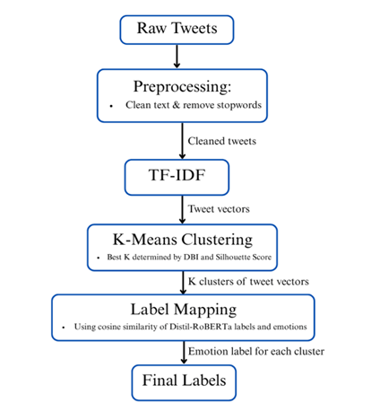
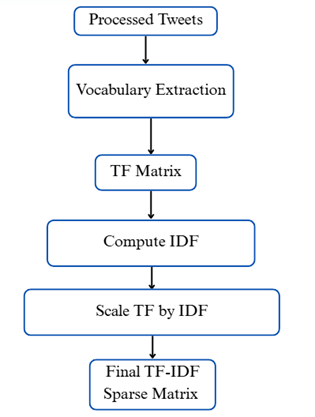
In this section, the algorithm used in this paper is described in detail. Unsupervised learning is employed to cluster and classify tweets based on multiple emotions. An overview of the procedure is illustrated in Figure 1.

2.1. Dataset Selection and Exploratory Data Analysis

Data are selected to experiment with whether the algorithm would perform well in the X ecosystem. They are collected from Kaggle (https://www.kaggle.com/datasets/parulpandey/emotion-dataset) and include 20,000 tweets from a real X environment across different topics. From this Kaggle source, 16,000 tweets are extracted, forming the primary dataset. To increase generalizability, the other 4,000 tweets form the second dataset used for model validation in Section 3.1.6.  All tweets are previously human-labeled; however, those labels are not used in the unsupervised pipeline but only as ground truth labels for external validation.

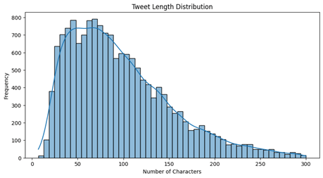
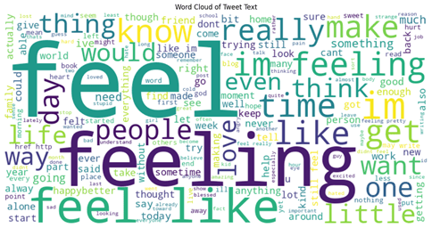
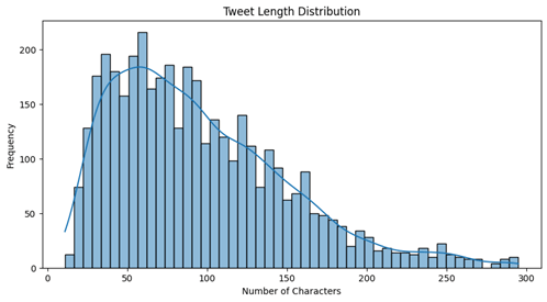
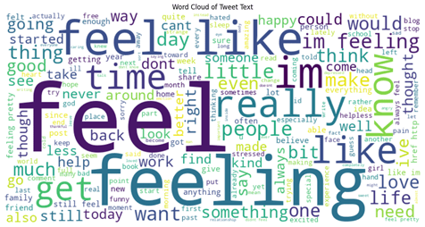
For the primary dataset of 16,000 tweets, exploratory data analysis reveals that 83.42% of the tweets are under 150 characters, as seen in the graph of tweet length distribution in terms of character numbers (shown in Figure 2).  The word cloud graph in Figure 3 shows that the most frequently appearing words are “feel”, “feeling”, and “feel like”. The second dataset of 4,000 tweets has a similar distribution of length and similar frequently-appearing words as shown in Figures 4 and 5. The frequently appearing word “feel” suggests that both datasets are concentrated on tweets that express emotions, which is ideal for testing sentiment analysis models.

2.2. Preprocessing

Further steps are performed to ensure the dataset is ready for the machine learning model to be implemented.

To prepare the raw tweet data for unsupervised analysis, each tweet is lowercased. Hyperlinks in the tweets that do not add meaning to the text are removed by removing strings of text that start with “https.” Twitter-specific texts, such as mentions and hashtags, are also removed.

A standard English stopword list from the NLTK (Natural Language Toolkit) library²⁰ is used to remove common grammatical words (e.g., the, is, and) that do not carry much emotional weight. After preprocessing, the textual input to the unsupervised model is composed of meaningful tokens and helps to avoid introducing noise into the model.

2.3. TF-IDF

After data preprocessing by cleansing the unnecessary information, the Term Frequency-Inverse Document Frequency (TF-IDF) algorithm^21,22 is used. This converts each tweet into a numerical vector that represents its semantic composition. TF-IDF tokenizes the data and assigns values based on the content and importance of the words. Hence, the vectors produced are sparse and weighted. This makes the data suitable for distance-based clustering of the vectors. Clustering assumes that the closer together two vectors are, the more similar the semantic information being represented is. The TF-IDF vectorizer process is summarized in Figure 6.

Each tweet is transformed into a TF-IDF vector that represents its semantic content using equation:

   

where t represents a certain token, d represents a tweet text, TF(t,d) represents Term Frequency of t in d, IDF(t, D) represents Inverse Document Frequency of t in the dataset D. And,

   

   

where DF(t) represents the number of tweets containing t, M represents the total number of tweets in the dataset D. Through these calculations, words are weighed by their importance and contribution to the semantic meaning of the text. Rare words will be weighed more heavily than common words.

2.4. K-Means Clustering

K-Means is used to separate the dataset into K clusters by minimizing the sum of squared distances within each cluster. K-Means Learning²³ is implemented through initialization, assignment, and iteration. Random tweets are chosen as the initial centroids, and the other tweet vectors are assigned to the nearest centroid based on Euclidean distance. Each centroid is calculated as the mean of the vectors in cluster k,

   

where represents the new centroid of cluster ,
represents the set of all data in cluster ,
and represents every data point that belongs to cluster .
The summation denotes the vector sum of all tweet vectors in cluster .

The system then takes iterative procedures to achieve the following optimization.

   

where represents the total number of clusters,
represents the centroid of cluster ,
represents the set of all data in cluster ,
and represents every data point that belongs to cluster .
The result is the cluster assignment of each tweet.

2.5.  Number of Clusters

Next, before finally forming the clusters, it is important to identify the optimal number of clusters, K, for the whole dataset. This is a hyperparameter that must be determined adaptively, instead of a parameter that the model could learn from the data. If there are too few clusters, semantically distinct groups could get blurred, and if there are too many clusters, similar tweets are fragmented across multiple clusters.

One of the commonly used quantitative measurements, Davies-Bouldin Index (DBI)²⁴, is adopted in this paper to identify the number of clusters best suited for a given dataset. The DBI is calculated independently for situations when the dataset is sorted into 2 to 30 clusters. The number of clusters that corresponds to the lower DBI score will be chosen to finally cluster the dataset, which indicates good cohesion and separation and therefore a superior cluster classification.

This DBI takes into account the within-cluster cohesion and the between-cluster separation of the clusters. For a dataset of K clusters, the score is defined as:

   

For each pair of clusters and , their similarity, , is defined as:

   

where and are the calculated average distances of data points in clusters and from their centers, respectively,

   

where represents the centroid of cluster Ci. is the distance between the centers of clusters Ci and :

   

For each cluster , find the maximum similarity to any other cluster. And DBI is equal to the average of all of the numbers calculated.

2.6.  Emotion Labeling 

Because the proposed unsupervised learning model was based on unlabeled data, the output clusters are not labeled with emotions. Emotion labeling is done through probabilistic inference using the DistilRoBERTa model²⁵ and cosine similarity. DistilRoBERTa is chosen because it is highly context-aware. The same phrase can be positive or sarcastic depending on the context. It calculates the softmax of representations of the tweets and outputs a probability of emotions, for example: {“sadness”: 0.72, “fear”: 0.11, “joy”: 0.010, “disgust”: 0.04, “anger”: 0.03}. The largest percentage is taken as the tweet’s most probable sentiment.

Then, an algorithm is used to find the main emotion for each cluster by comparing the centroid vector  of each K-Means generated cluster  with the average vector representations under each of the seven Distil-RoBERTa predicted emotion labels. Cosine similarity is used in this comparison. The equation of cosine similarity measures the angle between two vectors. It is the dot product of the two vectors divided by the product of their magnitudes. Thus, this algorithm links each unlabeled cluster to its most similar emotion. This ensures that the clusters are interpretable.

2.7. External Validation Metrics

DBI and other indices are used to measure the cohesion and separation of the unsupervised clustering outputs. These are internal validation metrics. Additionally, external validation metrics are used to measure the accuracy or effectiveness of the outputs. External validation metrics compare the clustering results with ground truth labels. In this paper, three external validation metrics are used: emotion classification accuracy of DistilRoBERTa, cluster purity, and Fowlkes-Mallows Index (FMI).

The emotion classification accuracy of DistilRoBERTa is presented as a simple percentage of DistilRoBERTa’s correct predictions compared to the ground truth labels.

The cluster purity measures how many data points from a single ground truth class are contained within a particular cluster, hence indicating the cluster’s “purity”. In this case, cluster purity is determined by finding in each cluster the ground truth emotion that most frequently appears and calculating the proportion. Mathematically, it is defined as the total number of points of the most frequently appearing emotion label in each cluster over the total number of data points. For a total of K clusters ,

   

where is the total number of data points,
is the set of ground truth classes,
calculates the number of data points in cluster that belong to the -th ground truth class ,
and indicates the number of data points in cluster that belong to the most frequently appearing ground truth class in cluster .

The Fowlkes-Mallows Index (FMI) is also an external evaluation metric to assess the similarity between the clustering results and the ground-truth class. It is the geometric mean of Precision and Recall as

   

where TP (True Positives) means the number of data pairs which are in the same sentiment labeling cluster and the same ground truth class, FP (False Positives) means the number of data pairs which are in the same labeling cluster but different ground truth classes, and FN (False Negatives) indicates the number of pairs which fall in different labeling clusters but in the same ground truth class.

2.8.  Chrome Extension Application

Furthermore, the proposed classification algorithm and emotional labeling model are applied as a Chrome Extension. This extension is able to label tweets with emotion categories using the above proposed unsupervised machine learning method. It operates on the user side via a Chrome extension embedded into the X.com webpage. It supports, as an add-on feature, a basic representation of classified emotion categories that is expressed as percentages on user profiles.

When the user visits any X page, a JavaScript file (content.js) will be injected into the API. This connects the machine learning model with the X page bidirectionally. It allows the model to extract tweets and the webpage to include the model’s emotion labeling outputs. Each tweet is extracted, made lowercase, tokenized, and excluded common English stopwords like “and,” “so,” and “the”. Each tweet is then transformed into a TF-IDF vector that represents its semantic content and then clustered using K-Means in the same manner discussed above. After each tweet on the page is labeled using DistilRoBERTa, the model samples the 60 most recent tweets of the Twitter profile the user is scrolling through to calculate the percentage of emotions this profile expresses, and then displays the data at the top of the profile page.

3. Results

3.1.  Experiments on Tweet Datasets

3.1.1. Number of Clusters

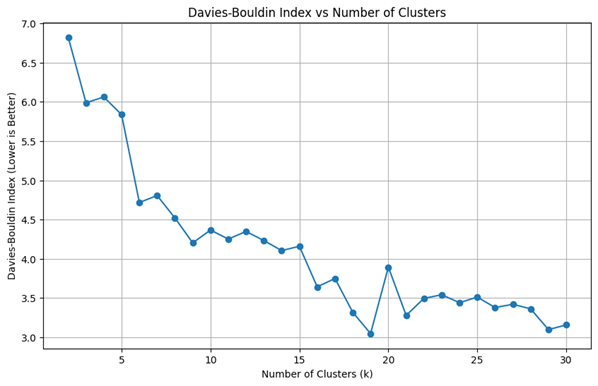
After applying TF-IDF vectorization on the 16,000-tweet dataset, the K-Means algorithm is implemented with different scenarios (splitting the dataset into 2 to 30 clusters), and their respective DBI score results against cluster numbers K are plotted in Figure 7. The candidate cluster number range is chosen from 2 to 30, as it aligns with psychological models suggesting that human emotions can be classified into up to 27 categories²⁶.

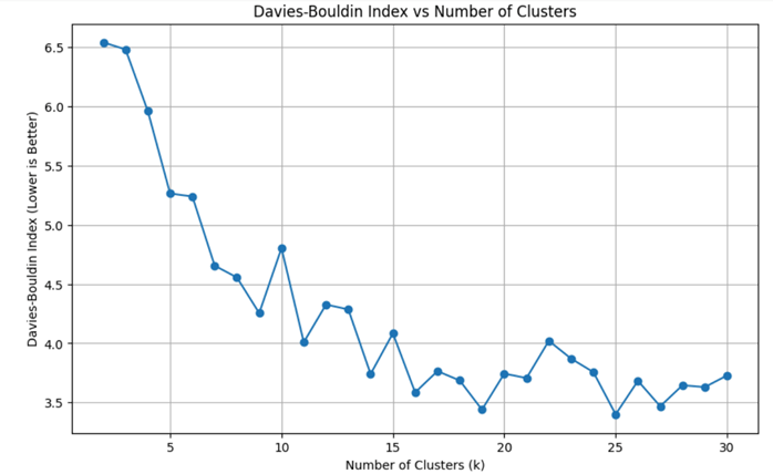
As shown in Figure 7, the DBI score decreases as the number of clusters K increases. When K increases from 2 to 7, the rate of change is high, and the DBI drops drastically, which indicates improving cluster differentiation. However, when K increases from 7 onwards, the rate of change is low, the DBI decreases slowly, and there are evident fluctuations. For example, at K =25, the DBI score (DBI₂₅=3.4003) is reduced by 26.9% against K =7 (DBI₇=4.6551) at the expense of cluster interpretability, comparing with the DBI score reduction of 28.8% for K =7 over K =2 (DBI₂=6.5392).

Therefore, choosing a K value that is near 7 ensures lower DBI and prevents over-clustering. To determine which value is more optimal, the silhouette score is computed for K =6 and K =7. The silhouette score²⁷ is another index that accounts for the cohesion and separation of unsupervised clusters. Using it in conjunction with DBI enhances the internal validity and accounts for outliers. For 7 clusters, the silhouette score is 0.0002, which is significantly worse than that for 6 clusters, at 0.0179. Hence, the number of clusters K =6 is used.

3.1.2. Clusters Visualization

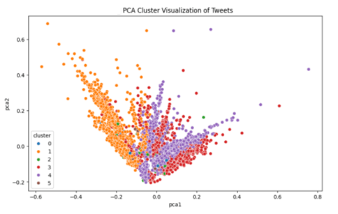
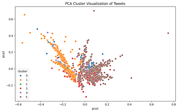
Then, a Principal Component Analysis (PCA) and a Hierarchical Clustering Dendrogram are done to visualize the six clusters. The PCA reduces the high dimensionality of the data to two axes with the most variance, PCA1 and PCA2. The hierarchical visualization is done through calculating the distance between pairs of data points and applying a merge algorithm to store and then display that information.

As shown in the PCA graph Figure 8, the orange cluster is packed tightly and clearly separated to the left. The purple cluster is also cohesive and has a tail shape. The red cluster is cohesive but overlaps with the purple one. The green, blue, and brown clusters overlap and are not very visible. They might capture outliers or reflect the limitation of PCA visualization in reducing high-dimensional vectors, a common problem with text-related data or complex vectors produced by TF-IDF. Overall, the PCA graph shows reasonable clustering with some structure.

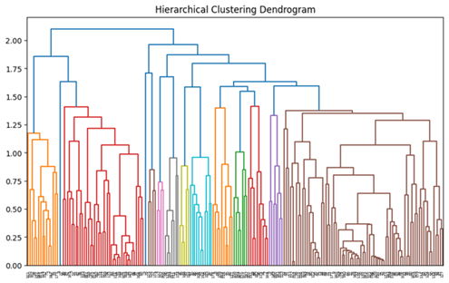
In the clustering dendrogram in Figure 9, there are long lines around height 2.0 near the upper bound. This means that the clusters are generally well-separated. At lower heights starting at 0.5, the lines become scattered and difficult to distinguish. This represents that between tweets within a larger cluster, there is closeness and similarity. These two positive observations contribute to the conclusion that the clustering is well separated at the high level and well-integrated at the micro level. However, exceptions to these two observations also exist, which could mean outliers or uneven cluster size. Further quantification is needed to ascertain these observations.

3.1.3. Calinski-Harabasz Index

To quantify the clustering quality, another index, the Calinski–Harabasz Index (CHI), was used. Like the DBI index, this value also represents how cohesive each cluster is and how separated clusters are from each other. In this paper, DBI is used as a preliminary way of determining the best number of clusters for K-Means. However, CHI is a more reliable indicator of the K-Means model’s outputs because it fits well with TF-IDF vectors. These vectors are in Euclidean space, which works well with the Euclidean distance calculations within CHI. DBI is the average similarity between clusters, and averages could be less sensitive to structure than CHI.

The CHI of 6 clusters for this dataset is found to be 118.73, which is higher than the threshold value for datasets of around 10,000 points of data. This means that the clusters are reasonably well separated and internally cohesive.

3.1.4. Emotion Labeling

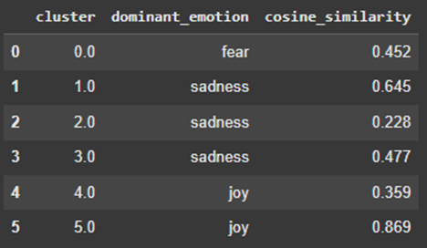
When the emotion labeler with the DistilRoBERTa model is run, the centroid vector of each cluster is compared with the average vector in each class of Distil-RoBERTa predicted emotion, and cosine similarity is used. The resulting interpretation of the dominant emotion for each cluster is shown in Figure 10.

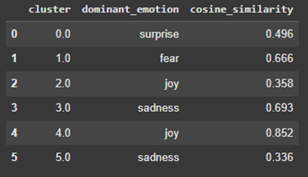
Of the 6 clusters, clusters 1, 3, and 4 have high cosine similarity scores, indicating that those clusters are more closely aligned with their labels of fear, sadness, and joy, respectively. Clusters 2 and 4 are both labeled as “joy,” and clusters 3 and 5 are both labeled as “sadness.” This could suggest that there are subtle differences between the “joy” expressed by tweets in cluster 2 and that expressed by tweets in cluster 4, for example.

Referring back to the PCA graph in Figure 8, cluster 4 demonstrates a strong, well-separated shape in the PCA plot, with a high cosine similarity of 0.852 to “joy”. In contrast, clusters 2 and 5 have low cosine similarities and a scattered shape in the PCA space, potentially indicating noise. Both clusters 3 and 5 are labeled “sadness,” but cluster 3 is emotionally denser and appears more cohesive than cluster 5 on the PCA graph. Similarly, clusters 2 and 4 are both called “joy,” but only cluster 4 shows strong alignment. Cluster 0, which is associated with “surprise,” is not well-defined, which may indicate that surprise has adjacent linguistic indicators as other emotions, and is harder to define.

Three example tweets from each cluster are extracted and presented in Table 1. The tweets align well with the emotion label and show interpretability.

Cluster	Emotion	Tweets
0	Surprise	i remember waking up feeling anxious and excited to read the bible its amazing how god will change your desires i am feeling amazed to see what god is doing new friends who aren t only amazing but get me who don t run and hide in a dark room unless i am there and they are joining me i had awesome workouts and feeling amazing
1	fear	i feel paranoid thinking about it just looking out the window and feeling my insomnia creep up on me i m drawing a blank as to what this is called to help me when i am feeling fearful or attacked i am concerned that my gut feeling about not dropping aol that quickly about not trusting verizon was not just paranoia
2	joy	i really like it a lot and think its a great fit for me and i love talking to the patients and trying to help them feel less nervous or at least that someone cares about them for a few minutes i feel honoured that my art is in someone s home and is being enjoyed on a daily basis i just love the feeling of something warmly hugging you and feeling so precious and small precious to someone something
3	sadness	i say this because she never truly gets a choice or the freedom to decide what to do with her life which makes it hard not to feel like she got the less dirty end of a really shitty stick i did feel like their relationship seemed a little rushed though i actually feel like i have been beaten up
4	joy	i feel is thankful for the lessons i m learning i feel so excited cause that means i get to skip classes i love running because i feel strong and powerful and totally in control
5	sadness	i feel like a mollusk repeatedly beaten with a wet cloth and stabbed times in the back just for the sake of it i want to tell everyone exactly how im feeling but as soon as i start to i feel ten times more pathetic and stop talking i often times feel lost here because all our friends seem to leave us and move away

3.1.5. External Validation Metrics

So far, the unsupervised pipeline has been evaluated by internal metrics such as DBI, CHI, and Silhouette score. External validation metrics are also employed to arrive at meaningful conclusions about the model’s accuracy and consistency in clustering and classification. The dataset is human-annotated. They are the ground truths that are used to determine the external validation metrics.

The emotion classification accuracy of DistilRoBERTa is calculated to be 83.05%. This value is determined by comparing the DistilRoBERTa predicted emotion labels to the human-annotated ground truth labels. The cluster purity is measured at 0.3392. The FMI index is calculated as 0.2872. This might be influenced by the overlap between different emotion classes, which creates noise, or the short text length, which makes vectors sparse.

3.1.6. Results on Second Dataset

The same pipeline is run on the other 4,000 tweets from Kaggle. This second dataset is a quarter the size of the former one, which tests whether the algorithm performs equally well on smaller datasets.  The number of clusters K is determined using the DBI score. The score trends downwards with some fluctuations as the number of clusters increases. As seen in Figure 11, the rate of change in DBI is substantial till K=6, hence K=6 is chosen. The DBI for 6 clusters in the second dataset is 4.7178, which is a slight improvement compared to the DBI for 6 clusters in the primary dataset at 5.2390.

PCA cluster visualization for six clusters on the 4,000-tweet dataset is shown in Figure 12, and its dominant emotion and cosine similarity for each cluster are shown in Figure 13.  As can be seen in Figure 12, clusters 1 and 5 stand out as they are compact and dense. Their emotional content is more distinctive and less ambiguous. They also rank highest in cosine similarity, which quantitatively supports this. Not only do these clusters group visually in PCA, but they are also highly aligned with the emotion labels. They are reliable representations of their labeled emotions. Clusters 2, 3, and 4 are more scattered in the PCA figure and have lower cosine similarity scores compared to other clusters with the same label. This could be due to variation or nuances within an emotion or noise in the tweet data, such as sarcasm. Also, some of the tweets in clusters 2, 3, and 4 might express multiple emotions and have Distil-RoBERTa labels that are more complicated, such as {“sadness”: 0.37, “fear”: 0.32, “joy”: 0.24, “disgust”: 0.07}. Cluster 0, which is labeled as “fear,” is noteworthy because it overlaps with other clusters in the PCA plot but does not share the same emotion label. The overlap may indicate the inherent emotional and semantic closeness between fear and other emotions, such as sadness.

Then, external validation metrics are calculated. The emotion classification accuracy of DistilRoBERTa versus ground truth labels is 81.61%, similar to what is obtained from the 16,000-tweet dataset. The cluster purity is measured at 0.3540.  The FMI index is calculated as 0.3174. Overall, the results obtained from the 4,000-tweet dataset have slight improvements from those obtained from the 16,000-tweet dataset. This is likely the result of the size difference between the datasets and the difference in data noise. The model’s performance is consistent in both larger and smaller datasets.

3.2. Comparative Analysis

3.2.1. Comparison with Unsupervised Methods

The unsupervised learning and labeling method proposed in this paper is comparatively analyzed with popular unsupervised clustering methods such as Agglomerative, DBSCAN, Spectral clustering, and UMAP + HDBSCAN. Experiments are run on the 16,000-tweet dataset. The same labeling approach is used. Cluster purity and FMI metrics are inspected and compared. The results are shown in Table 2. PCA cluster graphs are shown in Figures 14 to 17.

Method	Cluster Purity	FMI
Proposed Method	0.3392	0.2872
Agglomerative	0.3611	0.2291
DBSCAN	0.8041	0.1753
Spectral clustering	0.3369	0.4850
UMAP + HDBSCAN	0.5951	0.0544

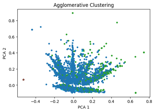
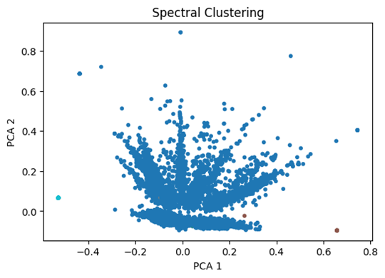
The proposed method’s FMI score is better than Agglomerative, DBSCAN, and UMAP+HDBSCAN, but lower than Spectral clustering. However, as the PCA graph for Spectral clustering shows in Figure 16, the clustering is extremely imbalanced, with one huge cluster, making the others indistinguishable. In terms of cluster purity, the proposed method has a lower result than DBSCAN and UMAP+HDBSCAN, and is close to Spectral and Agglomerative clustering. However, DBSCAN’s purity is inflated because, as the PCA visualization shows in Figure 15, it created a homogenous large cluster. The proposed method is likely more stable across different cluster sizes compared to DBSCAN and UMAP+HDBSCAN. 

3.2.2. Ablation Study

A comparative ablation study is conducted on individual components of the pipeline. First, a count vectorizer is used in place of the TF-IDF vectorizer. The resulting FMI was 0.3377, slightly better than that obtained by the proposed method, but the resulting cluster purity was worse at 0.2757. The higher FMI can be explained by the fact that the count vectorizer focuses on raw frequencies in its algorithm, which may help with detecting general similarity between texts but over-emphasizes common terms across different clusters, leading to fuzzy groupings. Hence, TF-IDF is still preferable. 

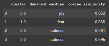
Second, the same pipeline is run on K=4 clusters instead of K=6 to test the output emotions. The cluster purity is 0.3353, which is slightly smaller than that of K=6. The resulting cluster labels and cosine similarities are displayed in Figure 18. Compared with the results in Figure 10 for K=6, while the 4-cluster method has a slightly higher average cosine similarity by 0.07 and slightly more cohesive clusters, the 6-cluster solution offers more complexity and nuance. It preserves the core clustering of the 4-cluster method, such as a strong joy cluster and a strong sadness cluster, indicating that the 6-cluster solution concurs with the overall classification of emotions. A higher K value might sacrifice cohesion marginally, but it compensates by potentially revealing subcategories within each broad sentiment label.

3.2.3. Literature Comparison

Abdalgader et al. performed a comprehensive evaluation on three unsupervised clustering methods (Partitional, Hierarchical, and Fuzzy clustering)²⁸ under the baseline condition of no sentence embedding measure. The experiments are run based on BERT and DistilRoBERTa models, respectively. The proposed method in this paper employs partitional clustering via TF-IDF + K-Means with the DistilRoBERTa model. It is implemented on the three datasets, SearchSnippets, AG News, and MR Dataset, provided by Abdalgader, and the performances are compared.

Model	FMI
Proposed Method TF-IDF+ K-Means +DistilRoBERTa	0.4786
Partitional clustering + DistilRoBERTa	0.290
Hierarchical clustering+ DistilRoBERTa	0.345
Fuzzy clustering+ DistilRoBERTa	0.134
Partitional clustering + BERT	0.302
Hierarchical clustering+ BERT	0.390
Fuzzy clustering+ BERT	0.225

Model	FMI
Proposed Method TF-IDF+ K-Means +DistilRoBERTa	0.4884
Partitional clustering + DistilRoBERTa	0.245
Hierarchical clustering+ DistilRoBERTa	0.233
Fuzzy clustering+ DistilRoBERTa	0.175
Partitional clustering + BERT	0.198
Hierarchical clustering+ BERT	0.302
Fuzzy clustering+ BERT	0.202

Model	FMI
Proposed Method TF-IDF+ K-Means +DistilRoBERTa	0.5370
Partitional clustering + DistilRoBERTa	0.297
Hierarchical clustering+ DistilRoBERTa	0.349
Fuzzy clustering+ DistilRoBERTa	0.289
Partitional clustering + BERT	0.313
Hierarchical clustering+ BERT	0.344
Fuzzy clustering+ BERT	0.282

As shown in Table 3 on the SearchSnippets dataset, the FMI score of the proposed method is evidently higher than that of the candidate unsupervised clustering algorithms in the literature. Compared to the best-performing result, Hierarchical clustering+ BERT with FMI of 0.390, this proposed method is 22.7% better. As shown in Table 4 on the AG News dataset, compared to the weakest-performing result, Fuzzy clustering with FMI of 0.175, the proposed method is approximately 2.8 times.

The results of the proposed method surpass the benchmark performance of the candidate algorithms in the literature running with DistilRoBERTa, demonstrating that the TF-IDF plus K-Means method improved the overall performance. In summary, a competitive FMI score shows that the proposed method is able to capture emotional structure meaningfully better.

Additionally, the SearchSnippet dataset has eight emotion classifications, the AG news dataset is labeled with four emotions, and the MR dataset is a binary emotion dataset. This proposed method’s success with all the datasets demonstrates that it can effectively classify texts into varying numbers of emotions. The SearchSnippet dataset is composed of results from search engines, the AG News dataset is a collection of news article titles, and the MR dataset is a set of reviews for movies and TV shows. These are different textual information from tweets, and the method’s success with classification on these three datasets shows a high level of generalizability to textual sentiment analysis beyond the Twitter environment.   

3.3.  Application as a Chrome Extension

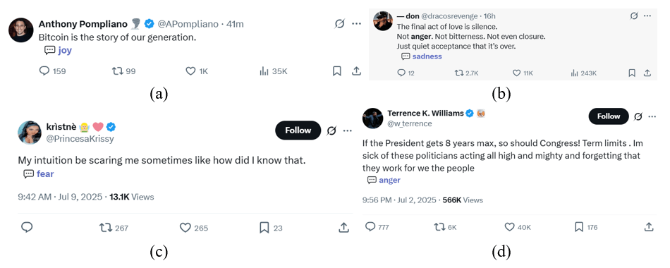
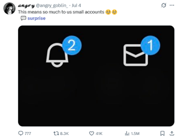
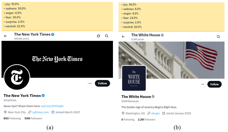
The proposed algorithm was successfully integrated into Google Chrome as an extension. When the user visits the X.com page, tweets are automatically analyzed using the TF-IDF plus K-Means module via JavaScript code. It extracts tweet contents in real-time, computes vectors, performs clustering, and then maps each cluster back onto an approximate emotional category through the process explained in Methods. Tests demonstrate that this labeling operates with minimal delay and provides the user with a sense of the sentiments of Twitter accounts. The resulting Chrome Extension program allows its users to see the emotion label of each tweet on the page and the percentage breakdown of the 60 most recent tweets made by a profile when the user clicks into it. Some screenshots of the model’s emotion labels of tweets are shown in Figure 19. Some screenshots of the model’s evaluation of a profile’s emotions based on recent tweets are shown in Figure 20.

Metrics	Result
Inference Latency (sec)	0.0738
Memory Usage (KB)	19.33
Peak Memory (KB)	33.39

Several key statistics relevant to the Chrome extension are measured and displayed in Table 6. These results suggest that the model is efficient in memory and time consumption. It is feasible for the Chrome extension prototype to be implemented in a real X environment.

However, CPU utilization sometimes reaches high peaks during the response timeframe, which may be due to the heavy computational demand of real-time TF-IDF vectorization. To mitigate this, optimizations such as precomputing TF-IDF centroids can be used.

Additionally, the model skips emoji-only or photo-only tweets. It deals with errors associated with the API limitations of Twitter or non-English language tweets by logging to the console. Methods such as fallback, retry, or notification mechanisms can be tried to better adapt the model to handling errors. 

The accuracy of the Chrome extension is verified with a human-labeled subset of 40 most recent tweets on the For You page of a new account. The topics range from politics and technology to jokes and celebrity gossip. The resulting accuracy is 26 correct out of 40, i.e., 65%. However, this is a small subset and is only a preliminary evaluation of the model’s performance.

4. Discussion

This study proposes, tests, and applies an unsupervised machine learning method for sentiment analysis on social media. This method clusters emotional language based on patterns rather than predefined labels, which enables more nuanced categorization, such as “fear,” “joy,” and “surprise,” making it applicable to the real-world online environment. The clustering results are supported by a good CHI score, PCA graph, Dendrogram, FMI score, and cluster purity. They suggest that this method can achieve meaningful clustering without the requirement for training on annotated datasets. When compared with typical unsupervised clustering models, the proposed method performs competitively. The application of this method with X data in real-time as a Chrome extension prototype demonstrates the potential for this model to be employed as a user-facing technology that helps users observe emotional trends. 

However, limitations must be acknowledged. First, the emotion-to-cluster mapping of emotional labels remains approximate, rather than concrete. Future iterations could integrate some supervision or external lexicons to increase precision.

Second, the system may not fully capture the emotions hidden in sarcasm, slang, emojis, or foreign cultures, which are prevalent on X. This is shown through some of the misclassifications of tweets in the Chrome Extension application. Though a library of common text abbreviations, such as LOL, OMG, NVM, etc., is used to account for some slang words, it is often difficult for the model to capture the levels of sarcasm. Many of the misclassifications the model produced could be linked to this limitation. For example, the tweet “NEVER TIRED OF WINNING” was encountered by the model in the Chrome Extension phase. Though this tweet expresses joy, it was labeled as sadness due to the lack of contextual interpretation of the word “tired”. Closely tied with context are emotionally ambiguous texts such as “she broke him emotionally,” which was labeled as anger despite having strong undertones of sadness. Sarcasm, context-dependent words, and tweets with complex emotion compositions could be detected by methods such as contradiction between emotion words in text and the expected label or the addition of contextual embeddings, such as GPT.

Third, the selection of the most optimal K value for clustering is done semi-manually via comparing the DBI and Silhouette scores and analyzing the trend of the graphs. Further optimization could approximate the DBI graphs as functions and mathematically compute the best K value through an adaptive calculation.

Fourth, when multiple clusters are labeled as the same emotion, it is difficult to understand whether it was the result of poor clustering or whether the model has discovered underlying nuances.

The methods of this paper are data-based, analytical, competitive, and scalable. The work done by this paper suggests that future research into unsupervised sentiment analysis could implement TF-IDF plus K–Means methods efficiently and effectively. Or, to improve upon this paper’s results and previous research, a hybrid system of both supervised and unsupervised components of sentiment analysis could be tried.

5. References

1. I.A. Albu and S. Spînu. Emotion detection from tweets using a BERT and SVM ensemble model.  2021 International Conference on Development and Application Systems (DAS), Suceava, Romania. 114-118 (2021). doi: 10.1109/DAS51855.2021.9439306. [↩]
2. Z. Qi, B. Zeng, and C. Zhang. Sentiment analysis of Twitter user comments based on Long Short-Term Memory networks. International Conference on Electrical Engineering and Intelligent Control (EEIC). 220 (2024). doi: 10.1049/icp.2024.3986. [↩]
3. R. Pradhan, G. Agarwal, and D. Singh. Comparative analysis for sentiment in Tweets using LSTM and RNN. International Conference on Innovative Computing and Communications, Singapore. 713-725 (2022). doi: 10.1007/978-981-16-2594-7_58. [↩]
4. I. Ameer, N. Bölücü, M. H. F. Siddiqui, B. Can, G. Sidorov, and A. Gelbukh. Multi-label emotion classification in texts using transfer learning. Expert Systems with Applications. 213, 118534 (2022). doi: 10.1016/j.eswa.2022.118534. [↩]
5. S. M. Mohammad and F. Bravo-Marquez. Emotion intensities in Tweets. Proceedings of the 6th Joint Conference on Lexical and Computational Semantics (SEM 2017), Vancouver, Canada. 65-77 (2017). doi: 10.18653/v1/S17-1007. [↩]
6. D. Demszky, D. Movshovitz-Attias, J. Ko, A. Cowen, G. Nemade, and S. Ravi. GoEmotions: A dataset of fine-grained emotions. Proceedings of the 58th Annual Meeting of the Association for Computational Linguistics (ACL). 4040-4054 (2020). doi: 10.18653/v1/2020.acl-main.372. [↩]
7. R. Plutchik. A general Psychoevolutionary theory of emotion. Emotion: Theory, Research, and Experience. 1, 3-33 (1980). H. Kellerman and R. Plutchik, Eds. New York, NY, USA: Academic Press. [↩]
8. J. A. Russell. A circumplex model of affect. Journal of Personality and Social Psychology. 39, 1161-1178 (1980). [↩]
9. E. Y. Bann. Discovering basic emotion sets via semantic clustering on a Twitter corpus. BSc dissertation / Univ. Bath (2012). [↩]
10. A. Agrawal and A. An. Unsupervised emotion detection from text using semantic and syntactic relations. International Conferences on Web Intelligence and Intelligent Agent Technology. 377-384 (2012). doi: 10.1109/WI-IAT.2012.170. [↩]
11. M. Unnisa, A. Ameen, and S. Raziuddin. Opinion mining on Twitter data using unsupervised learning technique. International Journal of Computer Applications. 148, 12-19 (2016). doi: 10.5120/ijca2016911317. [↩]
12. L. Zhu, A. Galstyan, J. Cheng, and K. Lerman. Tripartite graph clustering for dynamic sentiment analysis on social media. arXiv preprint.(2014). arXiv:1402.6010. [↩]
13. C. Argueta, E. Saravia, and Y. -S. Chen. Unsupervised graph-based patterns extraction for emotion classification. 2015 IEEE/ACM International Conference on Advances in Social Networks Analysis and Mining (ASONAM), Paris, France. 336-341 (2015). doi: 10.1145/2808797.2809419. [↩]
14. K. Darwish, P. Stefanov, M. Aupetit, and P. Nakov. Unsupervised user stance detection on Twitter. Proc. 14th International AAAI Conf. Web Social Media (ICWSM), Atlanta, GA, USA. 141-152 (2020). doi: 10.1609/icwsm.v14i1.7286. [↩]
15. S. Hiremath, S. H. Manjula, and K. R. Venugopal. Unsupervised sentiment classification of Twitter data using emoticons. 2021 International Conference on Emerging Smart Computing and Informatics (ESCI), Pune, India. 444-448 (2021). doi: 10.1109/ESCI50559.2021.9397026. [↩]
16. M. Nagayi and C. Nyirenda. Enhancing affinity propagation for improved public sentiment insights. arXiv preprint. (2024). arXiv:2410.12862. [↩]
17. M. Bibi, W. A. Abbasi, W. Aziz, S. Khalil, M. Uddin, C. Iwendi, and T. R. Gadekallu. A novel unsupervised ensemble framework using concept-based linguistic methods and machine learning for Twitter sentiment analysis. Pattern Recognition Letters. 158, 80-86 (2022). doi: 10.1016/j.patrec.2022.04.004. [↩]
18. K. Abdalgader, A. A. Matroud, and K. Hossin. Experimental study on short-text clustering using transformer-based semantic similarity measure. PeerJ Computer Science. 10, no. 4, e2078 (2024). doi: 10.7717/peerj-cs.2078. [↩]
19. S. Limboi. Comparison of data models for unsupervised Twitter sentiment analysis. Studia Universitatis Babeș-Bolyai Informatica. 67, 65-80 (2023). doi: 10.24193/subbi.2022.2.05. [↩]
20. S. Bird, E. Klein, and E. Loper. Natural language processing with Python. O’Reilly Media. (2009). [Online] https://www.nltk.org/. [↩]
21. G. Salton and C. Buckley. Term-weighting approaches in automatic text retrieval. Information Processing & Management. 24, no. 5, 513-523 (1988). [↩]
22. F. Sebastiani. Machine learning in automated text categorization. ACM Computing Surveys. 34, no. 1, 1-47 (2002). doi: 10.1145/505282.505283. [↩]
23. D. Xu and Y. Tian. A comprehensive survey of clustering algorithms. Annals of Data Science. 2, no. 2, 165-193 (2015). doi: 10.1007/s40745-015-0040-1. [↩]
24. J. Santos, M. Embrechts, and L. Moreau. On the use of Davies–Bouldin index to evaluate clustering algorithms. Information Sciences. 483, 78-101 (2019). doi: 10.1016/j.ins.2018.12.033. [↩]
25. Y. Liu, M. Ott, N. Goyal, J. Du, M. Joshi, D. Chen, O. Levy, M. Lewis, L. Zettlemoyer, and V. Stoyanov. RoBERTa: A robustly optimized BERT pretraining approach. arXiv preprint. (2019). arXiv:1907.11692. [↩]
26. A. S. Cowen and D. Keltner. Self-report captures 27 distinct categories of emotion bridged by continuous gradients. Proceedings of the National Academy of Sciences of the United States of America. 114, no. 38, E7900-E7909 (2017). doi: 10.1073/pnas.1702247114. [↩]
27. Y. Januzaj, E. Beqiri, and A. Luma. Determining the optimal number of clusters using Silhouette Score as a data mining technique. International Journal of Online and Biomedical Engineering. 19, no. 4, 174-182 (2023). doi: 10.3991/ijoe.v19i04.37059. [↩]
28. K. Abdalgader, A. A. Matroud, and K. Hossin. Experimental study on short-text clustering using transformer-based semantic similarity measure. PeerJ Computer Science.10, no. 4, e2078 (2024). doi: 10.7717/peerj-cs.2078. [↩]