Modeling Life Expectancy with Interpretable Machine Learning Approaches

Abstract

Objective: This study uses machine learning to predict life expectancy from diverse health, economic, and demographic indicators, while uncovering key drivers of population health using explainable machine learning techniques.
Methods: The dataset, obtained from Kaggle, underwent rigorous preprocessing, including outlier filtering, label encoding, and feature standardization. To ensure robust evaluation of models on time-ordered data, we used TimeSeriesSplit cross-validation. Three regression models were compared: Linear Regression, Multi-Layer Perceptron (MLP), and Random Forest. To enhance model transparency and identify critical features, we conducted a comprehensive feature attribution analysis using RF Feature Importance (MDI), Permutation Importance, and SHAP (SHapley Additive exPlanations) values.
Results: The Random Forest model achieved the best performance with a mean squared error (MSE) of 7.9763, with the MLP Regressor achieving an MSE of 174.9381 and Linear Regression achieving an MSE of 15.6540. The multi-method feature importance analysis consistently identified “Income composition of resources” as the single most critical predictor of life expectancy across all attribution methods.
Conclusion: These results suggest that ensemble tree-based models not only offer superior predictive accuracy but also provide meaningful insights into the drivers of life expectancy. Our findings underscore the value of explainable AI in public health analytics, offering decision-makers tools to better understand and act upon the complex socio-economic and health-related variables that influence longevity.

Keywords: life expectancy prediction, machine learning, public health analytics, SHAP values, socioeconomic indicators.

Introduction

Life expectancy is a core measure of population health, shaped by socio-economic, environmental, and healthcare factors^1‘2. Understanding what drives differences in life expectancy is crucial for informed public health policy, particularly in addressing disparities between developed and developing countries³. This study applies machine learning to predict life expectancy based on a diverse set of health and demographic indicators, ranging from adult mortality and infant deaths to alcohol use, immunization rates, and Gross Domestic Product (GDP).

We aim not only to build predictive models of life expectancy but also to uncover the most influential variables using explainable machine learning methods⁴. Drawing from a global dataset spanning multiple years, our work supports evidence-based health policy by highlighting key drivers of longevity.

Introduction to Life Expectancy as a Health Indicator

Life expectancy is a key indicator of a population’s overall health and well-being, reflecting the average number of years an individual is expected to live based on current mortality trends. It is shaped by a wide range of social determinants of health (SDOH), including socio-economic status, environment, and access to healthcare, making it critical for public health research and policymaking⁵. Governments and health organizations use life expectancy predictions to allocate resources, assess disease burden, and monitor development progress⁶.

Key Determinants of Life Expectancy

Socio-economic variables such as education levels, income distribution, and GDP have strong correlations with life expectancy⁷. Visualizations in this paper help illustrate these trends and contextualize the statistical analysis. Additional contributors include healthcare coverage, vaccination rates, and lifestyle factors like BMI and alcohol use^8‘9 . Infrastructural elements, such as sanitation and public health spending, also significantly impact longevity¹⁰.

Machine Learning Approaches in Life Expectancy Prediction

While traditional models like the Cox Proportional Hazards Model have been used in survival analysis, modern machine learning methods offer improved flexibility and performance. Linear regression assumes linearity, which may not always hold. In contrast, ensemble models like Random Forest can capture complex, nonlinear patterns, enhancing predictive accuracy¹¹. Neural networks, such as Multi-Layer Perceptrons (MLPs), further improve performance by learning hierarchical relationships from data¹².

Feature Importance and Explainability in Predictions

A major challenge in machine learning models is the interpretability of results. To address this, techniques such as SHapley Additive Explanations (SHAP) and Feature Importance Scores from Random Forest Models help identify the most influential factors driving predictions¹³. SHAP is a model-agnostic interpretability method that explains individual predictions by calculating the contribution of each feature using principles from cooperative game theory, specifically Shapley values, which fairly distribute the model’s output among all input features based on their marginal impact across all possible feature combinations. For instance, another study has shown that adult mortality, education levels, and HIV/AIDS prevalence consistently rank among the top determinants of life expectancy¹⁴.

Scope and Limitations

While this study draws on a comprehensive, multi-year dataset with global coverage, there are limitations. Some regions and populations may be underrepresented due to inconsistent or missing data, which could bias model performance. Additionally, the dataset includes only quantifiable health, economic, and demographic variables, potentially omitting cultural, political, or systemic influences that also could affect life expectancy. As such, the findings should be interpreted within the constraints of available data and modeling assumptions.

Governing Equations and Statistical Formulations

The general formulation of life expectancy prediction in a machine learning framework is expressed as follows:

   

where represents the predicted life expectancy, is the set of independent variables, (such as GDP, schooling, immunization rates), is the function approximated by the model, and is the residual error¹⁵.

For regression-based models such as Random Forest, the prediction is obtained by aggregating individual decision trees:

   

where represents the final predicted life expectancy, represents the number of decision trees in the Random Forest, is the prediction made by the ‘th individual decision tree in the forest for input features , represents the sum of all predictions from each of the individual decision trees, and ensures that the final prediction () is the mean of all tree predictions.

A Multi-layer Perceptron (MLP) is a type of neural network that consists of multiple layers of neurons. The general mathematical representation of an MLP is:

   

where is the predicted life expectancy, is the number of layers in the network, is the weight matrix for the final layer, is the bias term for the final layer, is the activation outputs from the previous hidden layer, and is the activation function (ReLU, sigmoid, softmax.)

For a hidden layer, the output is computed as:

   

Where is the activation outputs from layer , is the weights for layer , is the bias for layer , and is the activation function.

For an MLP with multiple layers, the information propagates forward from the input layer to the output layer:

Input Layer: (feature vector, e.g., GDP, schooling, immunization rates)

Hidden Layers: Each layer applies a weight transformation and an activation function:

   

Output Layer: The final transformation is applied:

   

Where is the input features, is the learned weight matrices that determine how each feature contributes to the output, is the bias terms that shift the activation function’s output, is the activation function (such as ReLU for hidden layers and softmax/sigmoid for output), and is the predicted life expectancy¹⁶.

Related Works

The current study is situated at the intersection of public health informatics and advanced machine learning, drawing upon established research in three critical domains: the application of predictive modeling for longevity, the empirical validation of socioeconomic determinants of health (SDOH), and the deployment of Explainable Artificial Intelligence (XAI) techniques to enhance model transparency.

Machine Learning for Health Outcome Prediction

Traditional epidemiological studies have historically relied on generalized linear models to predict health outcomes. However, recent literature demonstrates the superior performance and ability of ensemble machine learning methods to capture the complex, non-linear interactions inherent in public health data. Research comparing multiple machine learning approaches found that Random Forest achieved predictive accuracy of R² = 0.9423, substantially outperforming linear regression and decision tree methods¹⁷. Studies analyzing life expectancy based on immunization features and human development factors have demonstrated that Random Forest regression achieves superior performance with high r-squared values compared to other regression algorithms¹⁸.Comprehensive evaluations of multiple machine learning models have consistently demonstrated that ensemble methods, particularly Random Forest, achieve the highest performance for life expectancy prediction¹⁹. This application of advanced machine learning moves beyond mere correlation to provide high-fidelity forecasts crucial for resource allocation and policy planning.

Socioeconomic Determinants of Health

The findings of previous research, particularly the high feature importance assigned to the “Income composition of resources,” are strongly supported by foundational public health literature concerning SDOH. Research has established that SDOH have a greater influence on health than either genetic factors or access to healthcare services, with poverty being highly correlated with poorer health outcomes and higher risk of premature death²⁰. Studies examining societal health burden and life expectancy have found that experiencing poverty or near poverty imposed the greatest burden and lowered quality-adjusted life expectancy more than any other risk factor, with 8.2 quality-adjusted life years lost per person exposed over their lifetime²¹. The public health community has accumulated substantial evidence pointing to socioeconomic factors such as income, wealth, and education as the fundamental causes of a wide range of health outcomes²². The World Health Organization’s framework divides SDOH into structural determinants, including socioeconomic and political context, social class, and ethnicity, and intermediary determinants, such as material circumstances and behavioral factors, with social, economic, and political mechanisms contributing to socioeconomic position characterized by income, education, and occupation²³. The reliance of our model on these features reinforces the established understanding that developmental and economic factors are critical precursors to a population’s life expectancy.

Explainable Artificial Intelligence (XAI)

The ethical and practical necessity of model transparency in sensitive fields like public health is paramount. While ensemble tree methods boast high predictive power, they often function as “black boxes.” The utilization of XAI techniques, specifically SHAP (SHapley Additive exPlanations) and Permutation Importance, is crucial for translating complex model structures into actionable policy insights. SHAP is a model-agnostic interpretability framework based on Shapley values from cooperative game theory that calculates the weight of each feature’s contribution to the predicted outcome, offering theoretically sound, consistent, and locally accurate feature attributions. SHAP connects optimal credit allocation with local explanations using classic Shapley values from game theory, providing a game theoretic approach to explain the output of any machine learning model^13‘24. SHAP provides both local and global explanations and has the ability to detect non-linear associations, making it superior to alternative methods that are limited to local explanations only²⁵.

Permutation feature importance is a model-agnostic technique that measures the contribution of each feature to a fitted model’s statistical performance by randomly shuffling feature values and observing the resulting degradation of the model’s score²⁶. This method normalizes biased feature importance measures based on a permutation test and returns significance values for each feature and can be used together with any learning method that assesses feature relevance^27‘28. Unlike tree-based feature importance measures that can be biased toward high cardinality features and may overfit, permutation-based feature importance avoids these issues since it can be computed on unseen data and does not exhibit such bias²⁶. These methods ensure that the model’s accuracy is accompanied by trustworthy, transparent evidence for decision-makers.

Methods

Dataset Description

The dataset is publicly available on Kaggle under the title “Health and Demographics Dataset”²⁹. It contains data from 1,649 samples, with 22 features. Each sample represents each country’s statistics and life expectancy in various years from 2000 to 2014, allowing for a temporal analysis of life expectancy trends. The dataset captures the interplay between health factors, economic indicators, and demographic characteristics across different countries and years. The key objective of this dataset is to investigate the influence of various factors on life expectancy and explore how these variables interact to shape population health globally.

The dataset consists of the following key features:

Feature Name	Unit / Format	Definition
Country	Name (String)	Name of the country.
Year	Integer	The year of data collection.
Status	Developed/Developing	Development status of the country.
Life Expectancy	Years	The target variable representing the expected lifespan at birth.
Adult Mortality	Per 1,000 population	Probability of dying between ages 15 and 60.
Infant Deaths	Per 1,000 live births	Number of infant deaths within the first year of life.
Alcohol	Liters per capita	Average alcohol consumption.
Health Expenditure	% of GDP	Percentage of GDP allocated to health expenditure
Hepatitis B	%	Immunization coverage for Hepatitis B.
Measles	Cases per 1,000 population	Reported cases of measles.
BMI	Average Index	Average Body Mass Index of the population.
Under-Five Deaths	Per 1,000 live births	Mortality rate for children under five.
Polio	%	Immunization Coverage for Polio.
Total Health Expenditure	% of GDP	Total health spending as a fraction of GDP.
Diphtheria	%	Immunization Coverage for Diphtheria.
HIV/AIDS	%	Prevalence of HIV/AIDS
GDP	USD per capita	Economic output per person.
Population	Total Number	Total population of the country.
Thinness (1-19 years)	%	Prevalence of underweight individuals from 1-19 years
Thinness (5-9 years)	%	Prevalence of underweight individuals from 5-9 years
Income Composition of Resources	Composite Index	A composite index of income distribution and resource access
Schooling	Years	Average number of years of education.

Data Preprocessing

Categorical variables, such as Country and Status, were transformed using Label Encoding to convert them into numerical values suitable for machine learning algorithms. Label encoding was used because one-hot encoding would have created a very high-dimensional sparse feature matrix, which could reduce model efficiency and risk overfitting given the modest sample size. Label encoding allowed us to preserve all categories into a compact representation. Standardization was then applied using the StandardScaler from Scikit-learn to normalize the features, ensuring that each variable contributes equally to the model’s learning process²⁶. Data cleaning was performed using Z-score and interquartile range (IQR) filtering to remove outliers and ensure data quality. Furthermore, a sensitivity analysis was conducted by testing all combinations of Z ∈ (2.00, 2.25, 2.50, 2.75, 3.00) and IQR Multiplier ∈ (1.25, 1.40, 1.50, 1.6, 1.75). The optimal combination of filtering thresholds was selected based on the MSE performance of the models across all scenarios, ensuring the final dataset maximized model generalizability. The best thresholds were found to be a z-score of 3.0 and an IQR multiplier of 1.25.  These thresholds were chosen to retain the majority of the data while effectively eliminating extreme outliers.

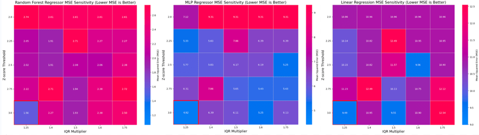
The results of this analysis, presented in Figure 1, demonstrate that the overall best model performance was achieved at the most aggressive filtering setting: a Z-score threshold of 3.0 and an IQR multiplier of 1.25. This combination resulted in the lowest MSE of 1.5628 for the Random Forest model, 4.9161 for the MLP, and 9.4885 for the Linear Regression model.

Following outlier removal, a crucial step was the assessment and mitigation of multicollinearity, a statistical phenomenon where highly correlated independent features can lead to unstable model coefficients. A Variance Inflation Factor (VIF) analysis was executed on the current feature set. This analysis identified severe multicollinearity issues, specifically involving the pairs of infant deaths with under-five deaths, and GDP with percentage expenditure. To stabilize the regression estimates, the features infant deaths and GDP were removed from the dataset because among the pairs, they had the highest VIF values. This feature selection step successfully reduced the maximum VIF score for all remaining predictors to an acceptable level (all VIF scores were 7.52 or lower), ensuring model stability and interpretability for subsequent training.

In preparation for model training, specific measures were taken to mitigate the risk of data leakage, a concern often present in panel datasets where strong, categorical grouping features exist. As the Country feature is known to have some predictive influence (as confirmed by subsequent feature importance analysis), standard random splitting would likely allow the model to learn country-specific patterns from the training set that are too unique to generalize, leading to an overly optimistic performance estimate.

To address this, a stratified splitting methodology was implemented. This approach ensures that the train and test sets are split based on the Country identifier, preventing a model from using a country’s identity as an indirect feature (data leakage) and forcing it to learn relationships that hold across different countries. This rigorous method ensures that predictive accuracy is based on the generalizability of the features, not on the model’s ability to memorize country-specific outliers or patterns.

This stratification constraint required that every country included in the final dataset possess a minimum of two samples to facilitate a proper split. Following the initial outlier removal, three countries were found to retain only a single data point. To maintain the methodological integrity of the country-stratified evaluation, these three rows were removed. The resulting clean dataset used for modeling and evaluation comprised of 1,576 samples.

The preprocessing pipeline was sequentially constructed to ensure data integrity and, critically, to prevent data leakage. Initially, although no missing values were present, an imputation step was prioritized as a foundational requirement. Next, all remaining categorical variables, including the highly predictive Country feature, underwent encoding to convert them into a numerical format, necessary for core scikit-learn operations. This encoded dataset was then immediately subjected to a stratified splitting methodology along the Country identifier, ensuring that each country’s data appeared in either the training set or the test set, but never both. This pre-split placement is essential to rigorously prevent data leakage, ensuring that subsequent feature engineering steps, specifically Scaling to standardize feature ranges and the subsequent Outlier Removal (using IQR and Z-score checks), are fitted exclusively on the training data. This ensures the test set remains an unbiased sample, validating the model’s true generalizability.

The table below shows the proportion of rows that were removed from preprocessing. There were no duplicate rows or missing values.

Metric	Value	Percentage of Original
Initial Row Count	1,649	100%
Rows Removed to Enable Stratification	2	0.12%
Rows Removed (z-score)	0	0%
Rows Removed (IQR)	71	4.30%
Total Rows Removed	73	5.64%
Final Row Count	1,576	95.57%

The target variable for prediction is Life Expectancy, representing the average number of years a person is expected to live. The features were selected based on their relevance to demographic, economic, and health factors influencing life expectancy. All available features except Life Expectancy were used to predict the target variable. These include a range of demographic, health, and economic indicators, which are all relevant for understanding life expectancy trends.

Data Visualizations

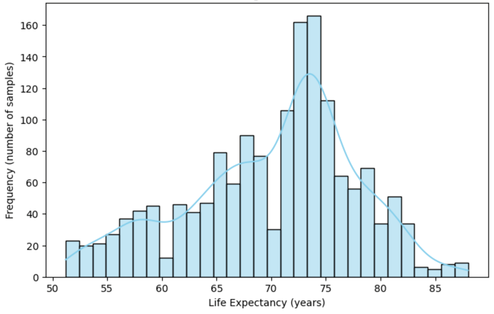
To better understand the distribution of life expectancy in the dataset, a histogram is presented in Figure 2. This histogram shows the distribution of life expectancy values after the data cleaning process. It reveals the spread and concentration of life expectancy values across the samples. The shape of the distribution can offer insights into the general life expectancy trends within the dataset.

Figures 3 and 4 show the distribution of life expectancy before and after cleaning.

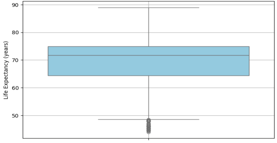
Figure 3 displays the distribution (median, IQR) of life expectancy values before the data cleaning process. The box plot highlights the presence of extreme outliers.

Figure 4 represents the distribution of life expectancy values (median, IQR) after the data cleaning process. The removal of extreme outliers is evident, resulting in a more compact and accurate representation of the data.

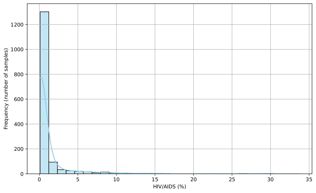
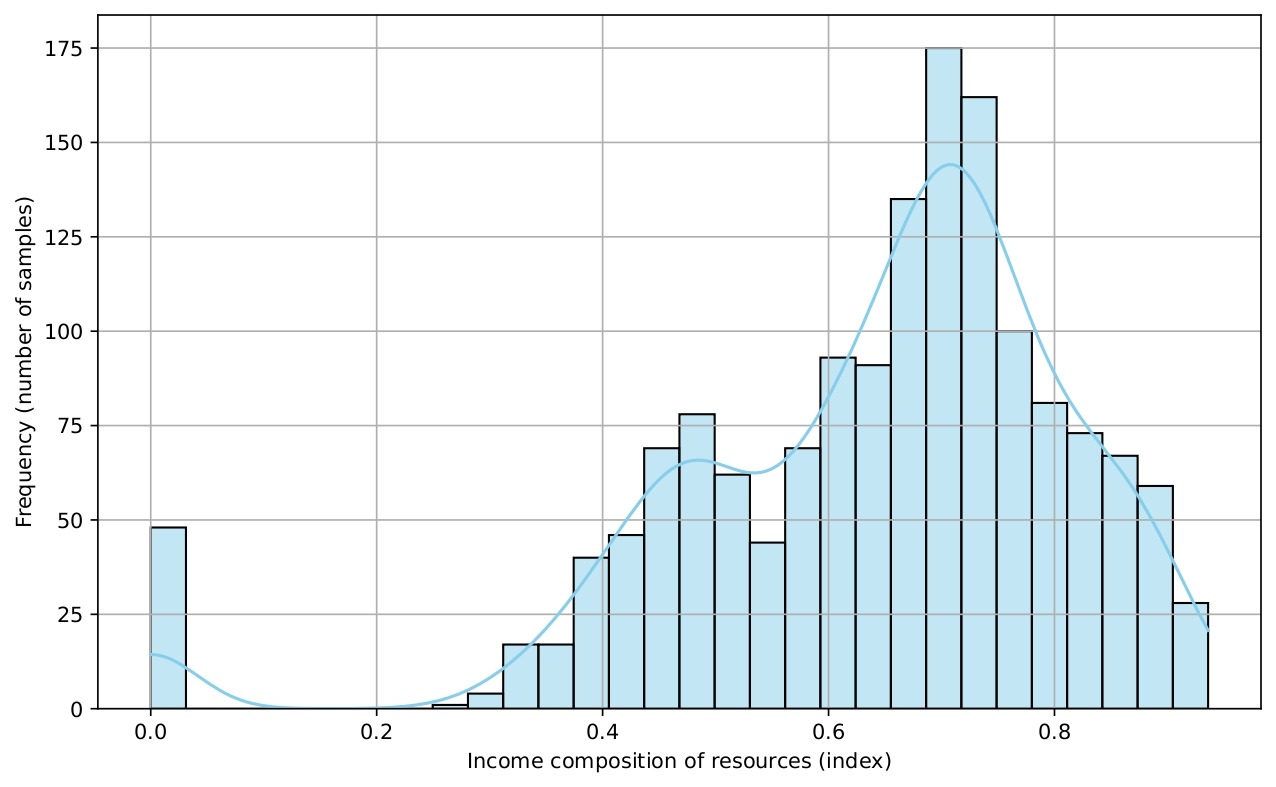
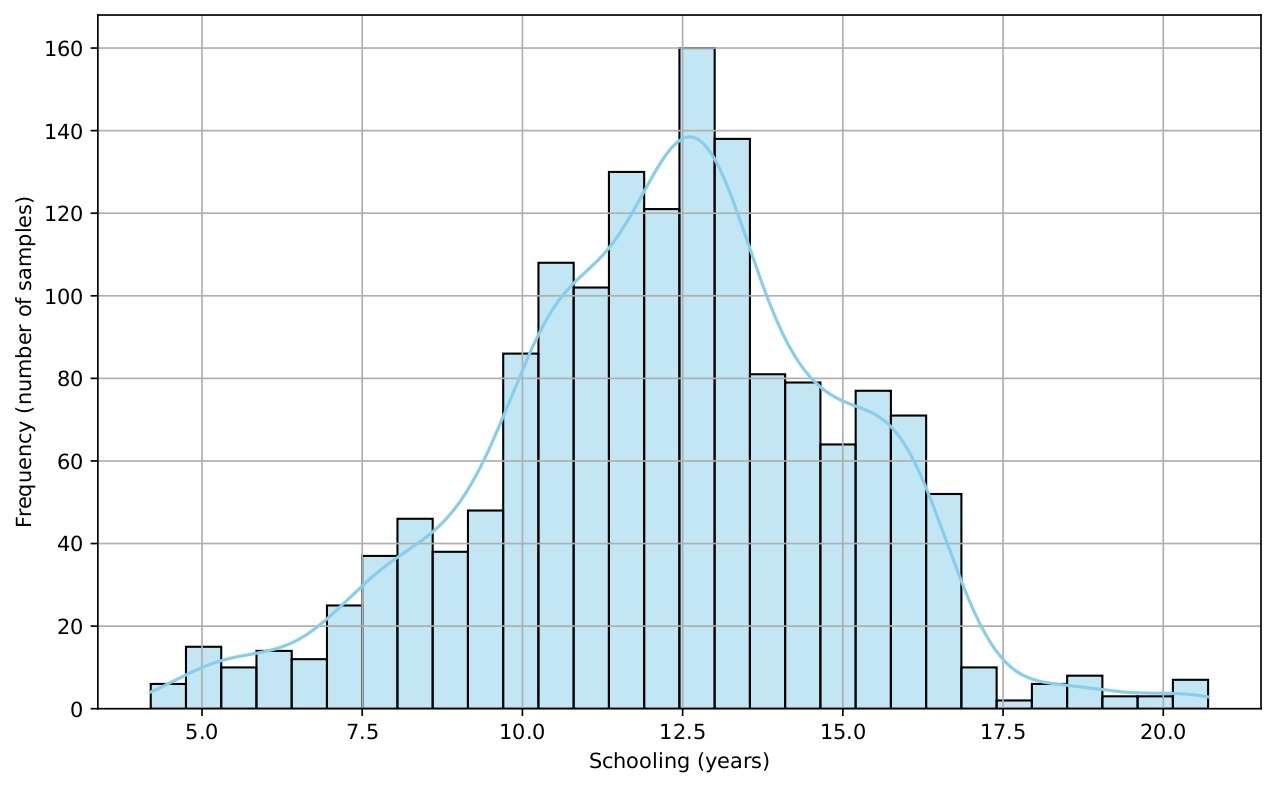
Several histograms are shown (Figures 5-9) to provide a visual overview of the key features that influence life expectancy. These distributions help illustrate the variation in the data for each important predictor (after cleaning).

Data Splitting

The cleaned dataset was split into training and testing sets using a 90:10 ratio, with 90% of the data allocated for model training and 10% for testing. This split was chosen to ensure that the model is trained on a sufficient amount of data while retaining enough samples for robust evaluation. Second, to provide a stable and robust estimate of the final model performance, a 5-fold Time Series Cross-Validation (TS-CV) was performed on the full cleaned dataset. The TS-CV approach accounts for the potential temporal dependency in the data.

Experimental Approach

The experimental approach focuses on training multiple regression models to predict life expectancy based on various features/variables. These models are evaluated using mean squared error (MSE) as the primary metric, which helps us assess the accuracy of each model in predicting the target variable, life expectancy.

• Linear Regression: This model was selected as a baseline due to its simplicity and interpretability, providing insight into the linear relationships between the features and the target variable.
• Multi-Layer Perceptron (MLP) Regressor: A neural network based regressor was chosen for its capability to model complex, non-linear relationships between the features and life expectancy.
• Random Forest Regressor: Given its flexibility and ability to handle complex interactions, the Random Forest Regressor was tested as a more powerful ensemble method.

The performance of the models was compared based on their MSE scores, and the Random Forest Regressor, which provided the best performance, was selected as the final model.

Linear Regression

Linear Regression is one of the simplest models and assumes a linear relationship between the input features and the target variable. It aims to find the best-fitting line that minimizes the squared difference between predicted and actual values.

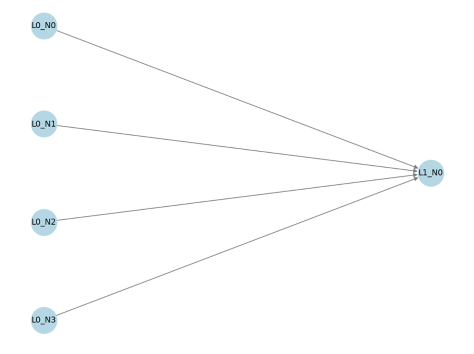
Figure 10 illustrates the architecture of a Linear Regression model. This model consists of an input layer (L0) with four input features, each representing a feature from the dataset. The input features are passed directly to the output layer (L1), which consists of a single output node that generates the predicted value for life expectancy. The model establishes a linear relationship between the input features and the output prediction, with no hidden layers, emphasizing its simplicity and direct nature.

Multi-Layer Perceptron (MLP) Regressor

MLP Regressor is a type of neural network model used to predict continuous values. It consists of multiple layers of neurons where each neuron in a layer is connected to every neuron in the next layer. The model uses activation functions such as ReLU to introduce non-linearity and is trained using backpropagation and gradient descent algorithms.

Model Architecture:

• Input Layer: The input features from the dataset are fed into the model.
• Hidden Layers: The MLP Regressor includes multiple hidden layers, with each layer having a set number of neurons. Hyperparameters such as the number of layers and neurons per layer were tuned during the grid search.
• Output Layer: The model outputs the predicted life expectancy for each test sample.

Hyperparameter Tuning: A grid search was used to tune the following hyperparameters:

• hidden_layer_sizes: Number of neurons in each layer (e.g., (100,50,25), (64,32,16,8)).
• activation: Activation function (ReLU or tanh).
• Optimization algorithm: The method used to update weights during training (Adam)
• L2 Regularization Coefficient (a): A coefficient applied as a penalty to prevent overfitting.

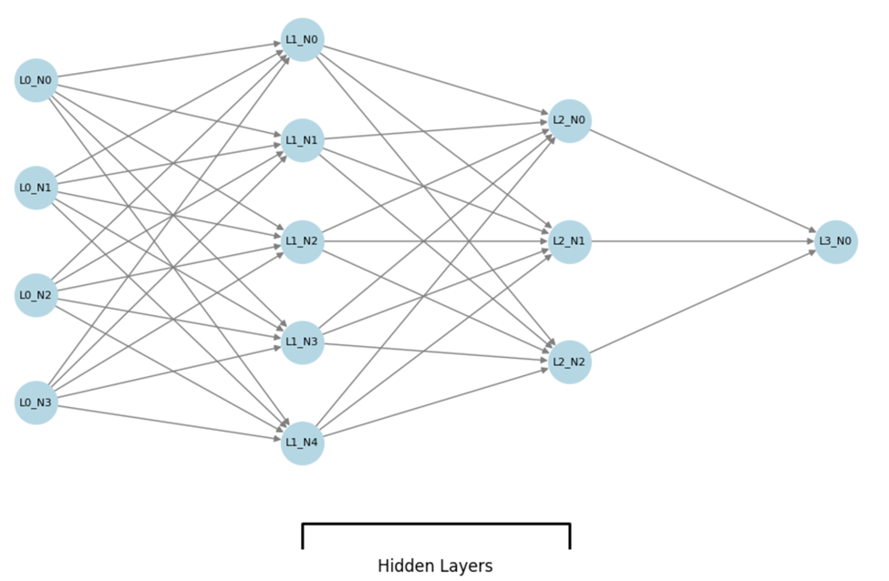
Figure 11 shows the basic architecture of an MLP Regressor. The MLP Regressor is a feedforward artificial neural network. The basic diagram consists of three main layers: the input layer, two hidden layers, and the output layer.

Input Layer (L0): The network begins with the input layer, which consists of four neurons (L0_N0 to L0_N3). Each neuron in this layer represents an individual feature from the input data. These features are fed into the network for processing.

●  Hidden Layers (L1 and L2):

○ The first hidden layer (L1) has five neurons (L1_N0 to L1_N4). Each neuron performs a weighted sum of the inputs from the previous layer (input layer), followed by an activation function (we used ReLU) to introduce non-linearity into the network.

○ The second hidden layer (L2) consists of three neurons (L2_N0 to L2_N2). Similar to the first hidden layer, these neurons process the output from the previous hidden layer using weighted sums and activation functions.

● Output Layer (L3): The network concludes with a single output neuron (L3_N0) in the output layer. This neuron produces the predicted value for the regression task (e.g., life expectancy), based on the transformed data from the hidden layers.

Random Forest Regressor

Random Forest Regressor is an ensemble method that uses multiple decision trees to make predictions. Each decision tree is built using a random subset of the data, and the final prediction is the average of all the individual tree predictions. This method is powerful in capturing non-linear relationships and interactions between features.

Model Configuration and Hyperparameter Tuning:

• n_estimators: The number of trees in the forest (50, 100, 200)
• max_depth: The maximum depth of each tree (10,20)
• min_samples_leaf: The minimum number of data samples in a leaf node (1, 2)
• max_features: The maximum number of features the model considers when searching for best split (sqrt, log(2), 1.0)
• random_state: Ensures reproducibility of the results.

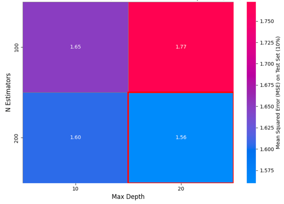
Figure 12 visualizes the resulting Mean Squared Error (MSE) for various combinations of two key hyperparameters: n_estimators (number of trees in the ensemble) and max_depth (maximum depth allowed for each tree).

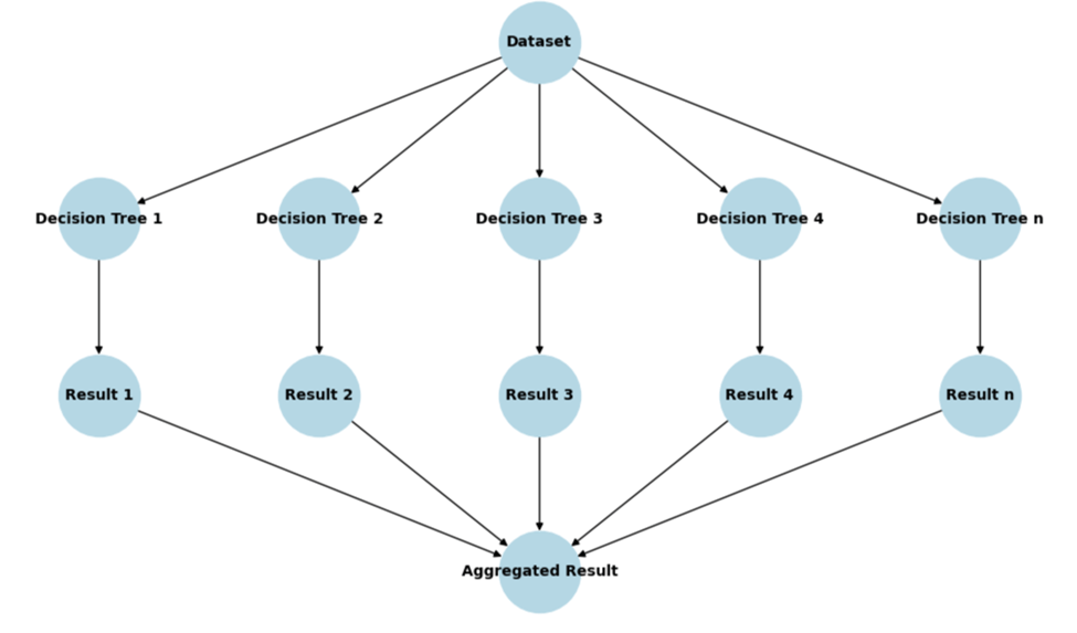
Figure 13 illustrates the flow of data through a Random Forest Regressor model. The input Dataset is positioned at the top, from which the data is passed to multiple decision trees (labeled Decision Tree 1 through Decision Tree n). Each decision tree generates an individual Result (labeled Result 1 through Result n). The final Aggregated Result is obtained by combining the individual results, typically through averaging, to produce the final prediction. This structure highlights the ensemble nature of Random Forest, where multiple decision trees work together to provide a robust prediction.

Ethical Considerations

This study used a publicly available, anonymized dataset aggregated at the country level, containing no personally identifiable information. Data usage complies with the terms set by the original data providers. Since the data is aggregated, individual privacy and confidentiality are preserved. Potential biases inherent in data collected from multiple countries and varying reporting standards were acknowledged as limitations that may affect model performance and generalizability. The predictive models developed here are intended for research purposes and should be applied responsibly, with awareness of their limitations. All data processing and modeling procedures were transparently documented to promote reproducibility.

Results

Model Performance and Evaluation

To provide a robust context for our complex machine learning models, we first established a simple, non-parametric Baseline model. This baseline predicts life expectancy solely based on the historical mean life expectancy of the corresponding Status observed in the training data. This ensures that the performance gains demonstrated by the complex models are genuinely due to learning from the feature set and not simply memorizing the Status averages.

The Random Forest Regressor demonstrated superior predictive performance for life expectancy compared to the Multilayer Perceptron (MLP) and Linear Regression models.

Model performance was evaluated using three key regression metrics:

• Mean Squared Error (MSE): This measures the average squared difference between the estimated and actual values. It heavily penalizes large errors, indicating the presence of significant outliers in the model’s predictions.
• Mean Absolute Error (MAE): This measures the average magnitude of the errors in a set of predictions, expressed in the same units as the dependent variable (in this case, years). It provides a more intuitive, linear measure of the typical prediction error.
• Coefficient of Determination (R²): This represents the proportion of the variance in the dependent variable that is predictable from the independent variables. An R² value close to 1 indicates that the model explains a high percentage of the variance.

The table below shows results for all three models and the baseline model with the 90:10 split.

Model	Mean Squared Error (MSE)	Mean Absolute Error (MAE)	R2
Status Mean Baseline Model	60.7350	6.4965	0.0903
Random Forest Regressor	1.5628	0.8882	0.9682
Linear Regressor	9.4885	2.4215	0.8437
Multi-Layer Perceptron (MLP)	4.9161	1.9332	0.9210

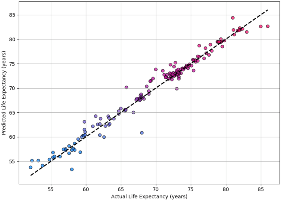
Figure 14 shows the predicted versus actual life expectancy values for the Random Forest Regressor on the test set. The close alignment of points along the diagonal line indicates high precision accuracy and low bias in the model.

To provide a more stable and robust estimate of model performance, a 5-fold Time Series Cross-Validation (TS-CV) approach was implemented on the final cleaned dataset. This method accounts for the potential temporal dependency within the data by ensuring that the training set always precedes the test set chronologically. Performance is reported as the mean and standard deviation of the Mean Squared Error (MSE), Mean Absolute Error (MAE) in years, and the Coefficient of Determination (R²) across the five sequential folds, thereby providing an indicator of both the average predictive accuracy and the stability of the model’s performance.

The table below shows the average results from all three models with the 5-Fold TS-CV approach.

Model	Mean MSE	Mean MAE	Mean R2
Random Forest Regressor	7.9763± 2.7826	2.1531 ± 0.5096	0.8630 ± 0.0344
Linear Regression	15.6540 ± 5.4840	3.1159 ± 0.6940	0.7305 ± 0.0699
Multi-Layer Perceptron (MLP)	174.9381 ±175.2422	6.1500 ± 3.7609	-1.8011 ± 2.7665

It is important to note the difference in magnitude between the MSE values reported in the fixed 90:10 split and the 5-Fold TS-CV approach. The substantially higher mean MSE values observed in the TS-CV analysis (e.g., Random Forest MSE moving from 1.5628 to 7.9763) are expected. This increase reflects the greater difficulty of predicting future values when the model has not been exposed to data from those later periods, which is the constraint imposed by the time-series splitting method. The lower MSE from the random fixed split is likely an overly optimistic estimate due to temporal leakage. Therefore, the TS-CV results provide the most reliable and unbiased assessment of the models’ out-of-sample predictive power over time.

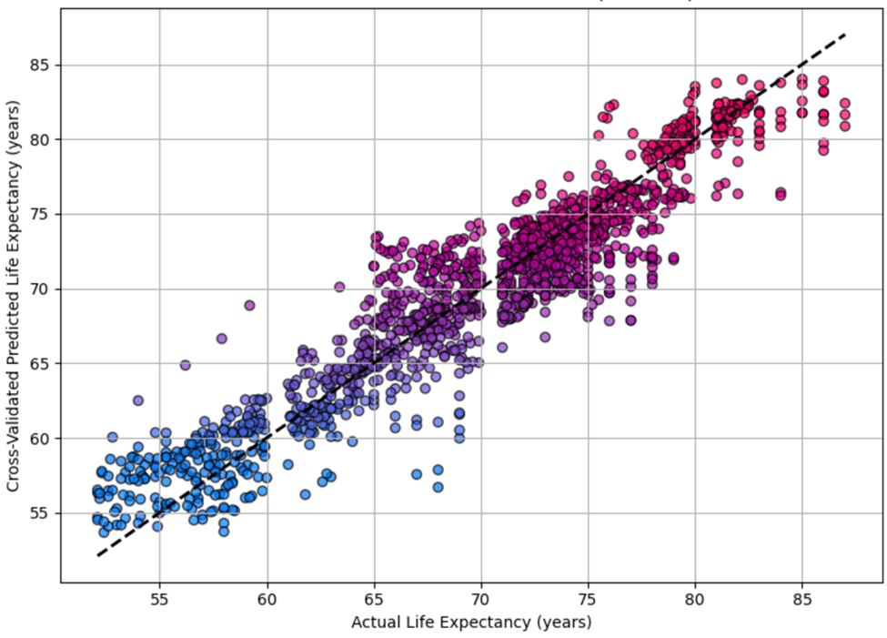
Figure 15 shows the predicted versus actual life expectancy values for the Random Forest Regressor on the test set with 5-Fold TS-CV.

Model Stability and Feature Transformation Analysis 

The primary model comparison established the Random Forest Regressor as the optimal choice for this problem. During the evaluation phase, we conducted an ancillary experiment to assess the impact of feature transformation on model stability and predictive performance.

Specifically, we applied a natural logarithm transformation to Population, the highly skewed predictor variable. This transformation (log_population) was tested across the three primary modeling approaches (Random Forest, Linear Regression, and MLP) using the established 5-Fold Time Series Cross-Validation methodology.

The table below shows the results from all three models with the 5-Fold TS-CV approach with the natural logarithm transformations to Population.

Model	Mean MSE	Mean MAE	Mean R2
Random Forest Regressor	8.2409 ± 2.5799	2.1495 ± 0.4722	0.8525 ± 0.0334
Linear Regression	24.3119 ± 17.7424	3.5997 ± 1.4475	0.5700 ± 0.2775
Multi-Layer Perceptron (MLP)	48.5846 ± 32.6405	4.2701 ± 2.0202	0.1460 ± 0.5159

The table above shows two observations regarding the impact of the log transformation:

• The MLP Regressor, which had failed on the original features, was successfully stabilized by the log transformation. This improved the model from a state of complete failure to a positive, albeit low, predictive score, reducing the error metrics (MSE and MAE) significantly.
• Crucially, the predictive performance of the best performing model, the RFR, was worse with the natural logarithm transformations than without the transformations.

Since the feature transformation did not provide a statistically significant or meaningful improvement for the optimal model, and the primary objective was maximizing predictive accuracy and minimizing error, we elected to discard the log-transformed features. Proceeding with the original scaled dataset maintains model simplicity and avoids unnecessary complexity without compromising the overall high predictive performance achieved by the Random Forest Regressor.

Correlation Analysis

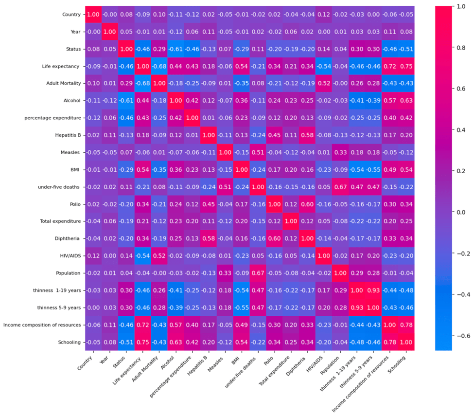
To better understand the underlying relationships between features and life expectancy, a correlation matrix was constructed (see Figure 16). Several features exhibit strong positive correlations with life expectancy, including Schooling (r=0.7464), Income Composition of Resources (r=0.7249), and BMI (0.5395). Conversely, features such as Adult Mortality (r=-0.6757) and HIV/AIDS prevalence (r=-0.5370) have strong negative correlations, reflecting their detrimental impact on life expectancy. These findings align with epidemiological knowledge and provide a useful baseline for interpreting the machine learning results.

Feature Importance from Random Forest Regressor

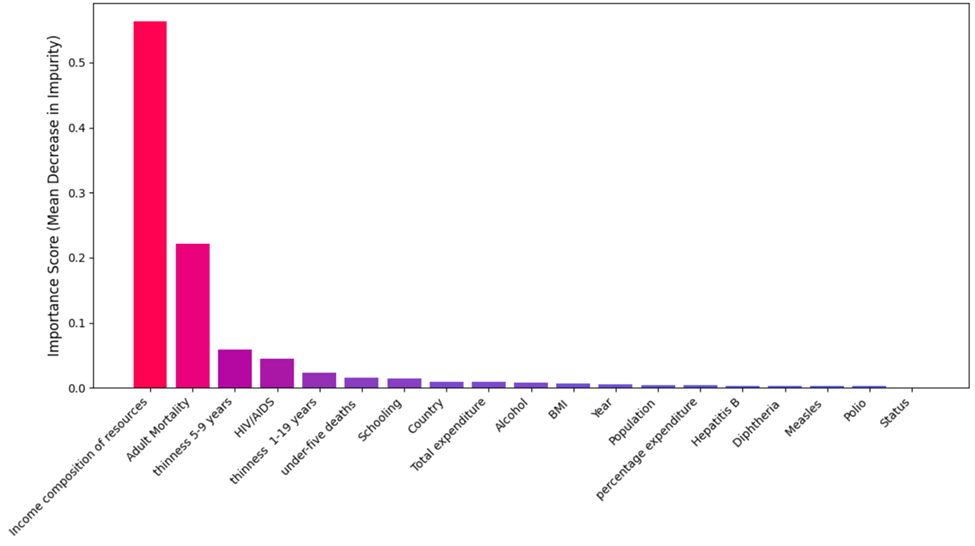
The feature importance values derived from the final, optimized Random Forest model are presented in Figure 17. To ensure these scores reflect the model’s generalized performance across time, the importance was calculated using the Gini Importance (Mean Decrease in Impurity) averaged across the five folds of the Time Series Cross-Validation (TS-CV) procedure.

The analysis emphasizes that Income Composition of Resources emerges as the most influential feature (importance = 0.5629) followed by Adult Mortality (= 0.2210) and Thinness, 5-9 years (= 0.0583). This averaging process provides a stable and robust ranking of feature contributions, demonstrating consistency regardless of the specific time window used for evaluation. This ranking supports the correlation findings and highlights the model’s focus on socioeconomic and health-related determinants.

Correlation Analysis and Feature Importance

The correlation matrix (Figure 16) and feature importance rankings from the Random Forest Regressor (Figure 17) together provide a more complete understanding of which factors drive life expectancy. While correlation shows how strongly and in what direction each feature is associated with life expectancy, feature importance highlights how much each feature contributes to the predictive power of the model.

The three most important features in the Random Forest model were:

• Income Composition of Resources (importance: 0.5629 correlation: +0.7249)
• Adult Mortality (importance: 0.2210; correlation: –0.6757)
• Thinness, 5-9 years (importance: 0.0583; correlation: –0.4584)

These variables not only rank highest in importance but also show strong correlations with life expectancy. This consistency strengthens confidence in the model’s ability to identify key drivers of health outcomes. Income Composition of Resources, for example, has both the highest importance and a strong positive correlation, indicating that access to income and resources is one of the most significant factors influencing longevity.

Although Schooling shows the highest positive correlation with life expectancy (+0.7464), its feature importance is relatively low (0.0146). This suggests that while education level is associated with life expectancy, its unique contribution to the model is limited, possibly due to overlap with other socioeconomic indicators like income.

Similarly, BMI and Alcohol consumption show moderate positive correlations (+0.5395 and +0.4431, respectively), but their importance values (0.0064 and 0.0086) are lower, indicating a smaller standalone predictive effect. Percentage expenditure (correlation: +0.4295; importance: 0.0036) also demonstrates this pattern, suggesting that while these variables relate to life expectancy, they may not add much unique information once the top features are accounted for.

In contrast, features with low correlations and low importances, such as Measles, Population, and Status, play minimal roles in both statistical and predictive terms.

Overall, the comparison confirms that the Random Forest model identified variables with both strong correlations and meaningful predictive value, especially those related to health risks and socioeconomic conditions.

SHAP Analysis: Model Interpretability

To gain deeper insight into how individual features affect predictions, SHAP (SHapley Additive exPlanations) values were computed. Figure 18 shows the overall magnitude of influence for each feature, calculated as the mean absolute SHAP value averaged across the five Time Series Cross-Validation folds. This averaging ensures a robust ranking of feature importance, independent of any single time-series split. Income Composition of Resources is confirmed as the dominant factor, followed by Adult Mortality and HIV/AIDS Prevalence.

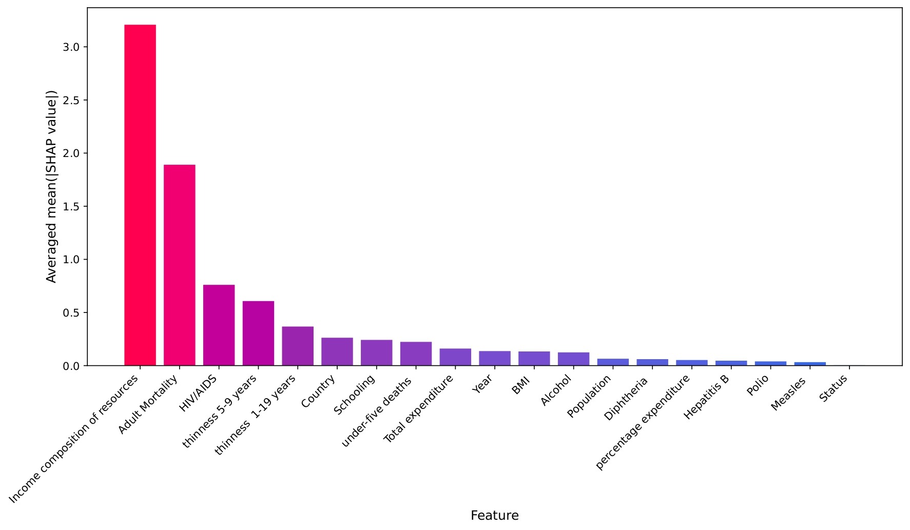
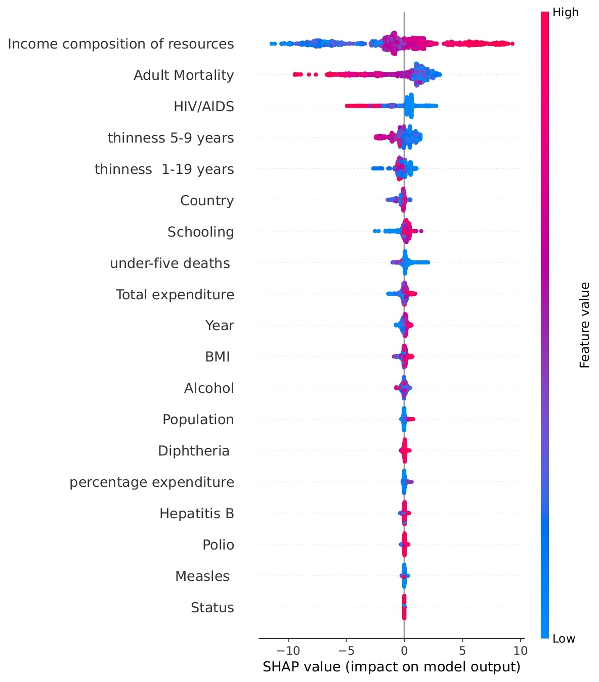
Figure 19 shows the total impact of each feature on the model’s Life Expectancy prediction, using data points concatenated from the five Time Series Cross-Validation test sets. The horizontal position indicates the SHAP value, representing the change in prediction from the base value. The color indicates the underlying feature value: Red points correspond to high feature values, and blue points correspond to low feature values. The resulting pattern shows, for example, that high Income Composition of Resources (red) drives the prediction right (higher Life Expectancy), while high Adult Mortality (red) drives the prediction left (lower Life Expectancy).

The SHAP analysis not only confirms the top features identified by the Random Forest model but also highlights some surprising patterns. For instance, thinness (both 5–9 and 1–19 years) and schooling, emerge as more impactful in shaping predictions than seemingly obvious metrics like BMI. This contrast is intriguing when compared to the correlation matrix. While BMI shows moderate positive correlations with life expectancy (r = 0.5395), its overall contribution to prediction is relatively low in the SHAP ranking. On the other hand, thinness, despite showing a strong negative correlation with life expectancy (r ≈ -0.4563 for ages 1-19, and r ≈ -0.4584 for ages 5-9), plays a more significant predictive role, likely because it serves as a proxy for broader issues like malnutrition and child health. Schooling, with a very strong correlation (r ≈ 0.7464), is both statistically and predictively powerful to a moderate extent, reinforcing its importance. However, alcohol consumption, with a moderate correlation (r ≈ 0.4431), shows less predictive utility than expected. These insights show that correlation alone does not fully capture the nuanced influence of features, and SHAP adds depth by quantifying both the size and direction of each variable’s impact on individual predictions.

Feature Importance Analysis

This section details the results of the feature importance analysis used to determine the predictive power of various health and economic indicators on Life Expectancy, as modeled by a Random Forest Regressor trained using a TimeSeriesSplit cross-validation strategy.

Methodology Overview

To establish the robust and unbiased ranking of predictive features, three distinct methods were employed and compared:

Method	Type	Metric	Key Advantage
Feature Importances (Random Forest)	Model-Specific (Random Forest)	Impurity Decrease	Fast and inherent to tree-based models
Permutation Importances	Model Agnostic (Test Set)	R2 Drop	Measures the direct impact on model performance (how much the prediction error increases)
SHAP (SHapley Additive exPlanations)	Model Agnostic (Test Set)	Mean Absolute SHAP Value	Provides a theoretically sound, fair attribution of contribution to the final prediction for each feature

Results and Interpretation

The analysis returned the following top feature importance rankings, shown in the table below.

Feature	RF Feature Importance	Permutation Importance (R2 drop)	Mean Absolute SHAP Value
Income Composition of Resources	0.5629	0.4115	3.2079
Adult Mortality	0.2210	0.2557	1.8903
HIV/AIDS	0.0446	0.0626	0.7601
Thinness (1-19 years)	0.0238	0.0155	0.3677
Thinness (5-9 years)	0.0583	0.0196	0.6074

A critical methodological step is to address the high RF Feature Importance value (0.5629) observed for Income composition of resources. This metric, calculated based on the Mean Decrease in Impurity (MDI), is known to favor highly continuous variables.

As a continuous variable with numerous unique values, Income composition of resources offers many possible splitting points during the Random Forest training process. This structural characteristic often leads to its RF Feature Importance score being significantly inflated and potentially misleading regarding its true influence when compared to features with fewer unique values (such as binary status indicators).

The high importance of the feature is confirmed by the consensus of the two unbiased, model-agnostic techniques:

• Permutation Importance: The Direct Performance Impact
• Permutation Importance quantifies the extent to which the model’s predictive accuracy suffers when a single feature’s values are randomly shuffled on the test set.
• Income Composition of Resources shows the greatest drop in model performance, with an R2 reduction of 0.4115. This indicates that the model relies most heavily on this feature to maintain its overall predictive power.

SHAP Values: The Attribution of Influence

• SHAP Values provide the most rigorous metric by fairly distributing the change in prediction from the baseline model across all input features. This model is crucial for interpreting complex, non-linear models like Random Forests.
• The Mean Absolute SHAP Value for Income Composition of Resources is 3.2079. This means that, on average, the presence of this feature shifts the predicted Life Expectancy value by approximately 3.2079 years (either positively or negatively.)
• The significant gap between the top-ranked feature and second-ranked feature, Adult Mortality (1.8903) provides the clearest, theoretically sound evidence that Income Composition of Resources is the single most dominant factor in determing the final predicted life expectancy.

Conclusion

The analysis provides strong evidence to strengthen the claim that Income composition of resources is the most influential feature in predicting life expectancy outcomes.

Despite the inherent statistical bias of both the RF Feature Importance metric favoring continuous predictors, the two robust, non-parametric methods (Permutation Importance and SHAP) both independently rank Income Composition of Resources as the most critical factor. Its consistent superiority across all three metrics confirms its role as the dominant economic and health predictor in the final model. This strongly supports the hypothesis that socioeconomic factors related to a country’s resource composition are the primary driver of life expectancy outcomes, even when compared against direct mortality and disease indicators.

Ablation Study: Validating Feature Importance

To confirm the necessity and robustness of the top five predictive features identified via SHAP and Gini importance, an ablation study was conducted. This analysis compares the performance of the full model against two segregated feature subsets using the established 5-fold Time Series Cross-Validation (TS-CV) methodology.

The feature subsets tested were:

• The Core Feature Set (Top 5): Features identified as dominant predictors, which were Income Composition of Resources, Adult Mortality, HIV/AIDS, Thinness (1-19 years), and Thinness (5-9 years)
• Ablated Feature Set (Other): The remaining 16 features from the dataset.

Model	Feature Count	Mean MSE	Mean MAE	Mean R2
Full Random Forest Regressor	19	7.9763 ± 2.7826	2.1531 ± 0.5096	0.8630 ± 0.0344
Core Features (Top 5)	5	6.8937 ± 1.3322	1.9301 ± 0.2698	0.8782 ± 0.0210
Ablated Features (others)	16	26.4754 ± 3.0740	4.1426 ± 0.4499	0.5329 ± 0.0435

The Ablated Feature Set (16 features) demonstrated extremely poor performance, yielding a Mean MSE of 26.4754 and a Mean MAE of 4.1426 years. This error is more than double the Mean MSE of the Full Model, confirming that these 16 features contain negligible predictive signal relevant to Life Expectancy and are highly dependent on the information carried by the core features. The high MSE relative to MAE also suggests this set produced predictions with several severe errors.

The most significant finding is the performance of the Core Feature Set of the top 5 features. By using only the top five predictors, the model not only maintained performance but outperformed the Full Model, achieving a Mean MSE of 6.8937 and a Mean MAE of approximately 1.9301 years. This 13.5727% reduction in MSE with a reduction in feature count from 21 to 5 indicates that the eliminated features were acting primarily as noise, degrading the generalization capabilities of the Full Model. The Core Feature Set successfully isolated the signal, resulting in a simpler, faster, and more accurate predictive model. This outcome robustly validates the use of the top five features for any practical deployment or further analysis.

Discussion

The Random Forest model’s superior performance highlights its ability to capture complex relationships in health and demographic data. The alignment of correlation analysis, feature importance, and SHAP explanations confirms the consistency of key life expectancy determinants.

Income Composition of Resources, reflecting socioeconomic conditions, emerged as the most influential feature, reinforcing the role of economic and social factors in population health. The strong negative effects of HIV/AIDS prevalence and Adult Mortality on life expectancy align with established public health findings.

SHAP analysis adds interpretability by illustrating how features impact individual predictions, revealing variation across countries and years. It also uncovers the relevance of features like schooling, alcohol consumption, and thinness, which show stronger model influence than more obvious metrics like BMI. For instance, schooling, though only moderately ranked by model feature importance, has a high SHAP impact and correlation with life expectancy, likely due to its long-term influence on health behaviors and access to care. Alcohol consumption, while generally viewed negatively, may act as a proxy for cultural or socioeconomic patterns. Thinness, especially in young children, strongly signals malnutrition and systemic health deficiencies, making it a more impactful predictor than BMI.

These findings show that feature importance is not solely about correlation strength but also about a feature’s unique and consistent contribution to predictive performance. Combining performance metrics, statistical relationships, and SHAP-based interpretability enables a deeper understanding of life expectancy drivers, supporting informed public health planning.

Our analysis provides clear guidance for public health policy. Socioeconomic interventions that reduce inequality and expand access to resources stand out as the most impactful levers for increasing longevity. Similarly, targeted health programs addressing adult mortality and infectious disease (particularly HIV/AIDS) can deliver substantial gains. Education and early-life nutrition policies also emerge as high-yield investments, given their consistent influence on life expectancy. These findings suggest that governments and international organizations should pursue multi-sectoral approaches that simultaneously address socioeconomic inequities, strengthen healthcare systems, and invest in long-term determinants such as schooling and child health.

Among the tested models, Random Forest achieved the lowest MSE (7.9763), outperforming MLP (174.9381) and Linear Regression (15.6540), demonstrating its robustness and interpretability. SHAP plots further clarify the model’s decisions, aligning results with public health priorities and improving transparency.

Limitations

Despite the robust methodology, the present study contains certain limitations that warrant consideration for future research:

Although the study used TimeSeriesSplit for chronologically appropriate validation, the Random Forest Regressor does not explicitly model the inherent time-series characteristics of life expectancy data (e.g., autocorrelation, long-term trends, or lagged effects). The manuscript currently fails to discuss these time-series characteristics and other potential temporal dependencies, which are essential for comprehensive analysis of longevity. Future work would significantly benefit from exploring sequential models, such as Autoregressive Integrated Moving Average (ARIMA) or Recurrent Neural Networks (RNNs) like LSTMs, to better capture and extrapolate these complex temporal dynamics.

The reliance on country-level, yearly aggregated data limits the ability to capture specific intra-country regional disparities or sub-annual changes in health policy effectiveness.

The high correlation between several socio-economic features (e.g., Income composition of resources, Schooling) makes it challenging for any model to strictly isolate the causal effect of one over the other. While SHAP offers attribution, it does not confirm causality.

While Permutation Importance and SHAP are powerful tools, they are sensitive to the correlation structure of the input data, meaning highly correlated features may split their attribution, potentially understating the overall contribution of the socioeconomic cluster.

Conclusions

This research successfully employed a TimeSeriesSplit-validated Random Forest Regressor to predict life expectancy, achieving high accuracy (MSE 7.9763) and demonstrating the superior fit of ensemble models for public health outcomes.

The primary conclusion, established through a rigorous consensus among MDI, Permutation, and SHAP analyses, is that Income composition of resources is the single most critical predictor of life expectancy. This finding strongly validates the core tenets of public health theory, emphasizing that investments in fundamental socio-economic and developmental factors yield the greatest returns in terms of population longevity. The framework developed here, which mandates the use of multiple explainable AI methods (SHAP and Permutation Importance) to validate the feature hierarchy, provides a template for future public health analytics. By offering transparent and meaningful insights into complex models, this approach allows decision-makers to prioritize policies that target structural determinants, such as education and economic stability, to achieve the most significant and sustained gains in global life expectancy. Future work should focus on leveraging higher-resolution, sub-national data and employing causal inference models to better disentangle the complex relationships within the highly correlated cluster of socioeconomic drivers.

Reproducibility Statement

The data is publicly available at Kaggle²⁹. The preprocessing and modeling code has been made publicly available at the following link: https://github.com/sohamathavale10-hue/Interpretable-ML-Health-Data-Prep. Due to the heavy analysis, we have used AI to organize and generate comments to benefit the reader and make our code more easily reproduceable.

References

1. World. Social determinants of health. World Health Organization. 2019,  https://www.who.int/health-topics/social-determinants-of-health. [↩]
2. National Research Council (US) Panel to Advance a Research Program on the Design of National Health Accounts. Defining and measuring population health. National Academies Press (US). 2010, https://www.ncbi.nlm.nih.gov/books/NBK53336/ [↩]
3. G. Miladinov. Socioeconomic development and life expectancy relationship: evidence from the EU accession candidate countries. Genus. Vol. 76 (2), 2020, https://doi.org/10.1186/s41118-019-0071-0. [↩]
4. M. Nishi, R. Nagamitsu, S. Matoba. Development of a prediction model for healthy life years without activity limitation: national cross-sectional study. JMIR Public Health Surveill. Vol. 9, 2023, https://doi.org/10.2196/46634. [↩]
5. C. D. Mathers, G. A. Stevens, T. Boerma, R. A. White, M. I. Tobias. Causes of international increases in older age life expectancy. Lancet. Vol. 385 (9967), pg. 540–548, 2015, https://doi.org/10.1016/s0140-6736(14)60569-9. [↩]
6. World Health Organization. World health statistics 2020: monitoring health for the SDGs, sustainable development goals. World Health Organization, 2020, https://www.who.int/publications/i/item/9789240005105. [↩]
7. S. H. Preston. The changing relation between mortality and level of economic development. Population Studies. Vol. 29 (2), pg. 231–248, 1975, https://doi.org/10.2307/2173509. [↩]
8. D. E. Bloom, D. Canning, J. Sevilla. The effect of health on economic growth: a production function approach. World Dev. Vol. 32 (1), pg. 1–13, 2004, https://doi.org/10.1016/j.worlddev.2003.07.002. [↩]
9. S. Lim, T. Vos, A. Flaxman, G. Danaei, K. Shibuya, H. Adair-Rohani. A comparative risk assessment of burden of disease and injury attributable to 67 risk factors and risk factor clusters in 21 regions, 1990–2010: a systematic analysis for the global burden of disease study 2010. Lancet. Vol. 380 (9859), pg. 2224–2260, 2012, https://www.thelancet.com/journals/lancet/article/PIIS0140-6736(12)61766-8/abstract. [↩]
10. M. Kabir. Determinants of life expectancy in developing countries. J Dev Areas. Vol. 41(2), 2008, https://ideas.repec.org/a/jda/journl/vol.41year2008issue2pp185-204.html. [↩]
11. L. Breiman. Random forests. Mach Learn. Vol. 45 (1), pg. 5–32, 2001, https://doi.org/10.1023/a:1010933404324. [↩]
12. Y. LeCun, Y. Bengio, G. Hinton. Deep learning. Nature. Vol. 521 (7553), pg. 436–444, 2015, https://doi.org/10.1038/nature14539. [↩]
13. S. Lundberg, Su-In Lee. A unified approach to interpreting model predictions. Advances in Neural Information Processing Systems. Vol. 30, 2017, https://doi.org/10.48550/arXiv.1705.07874 [↩] [↩]
14. D. Cutler, A. Deaton, A. Lleras-Muney. The determinants of mortality. ​​Journal of Economic Perspectives. Vol. 20 (3), pg. 97–120, 2006, https://doi.org/10.1257/jep.20.3.97. [↩]
15. T. Hastie, R. Tibshirani, J. Friedman. The elements of statistical learning: data mining, inference, and prediction, second edition. Springer Series in Statistics 2009, https://doi.org/10.1007/978-0-387-84858-7 [↩]
16. S. Haykin. Neural networks: A comprehensive foundation. 2006, https://cdn.preterhuman.net/texts/science_and_technology/artificial_intelligence/Neural%20Networks%20-%20A%20Comprehensive%20Foundation%20-%20Simon%20Haykin.pdf [↩]
17. R. Dolgopolyi, I. Amaslidou, A. Margaritou. Interpretable machine learning for life expectancy prediction: a comparative study of linear regression, decision tree, and random forest. 2025. https://doi.org/10.48550/arXiv.2510.00542. [↩]
18. A. Lakshmanarao, A. Srisaila, T.S.R. Kiran, G. Lalitha, K.V. Kumar. Life expectancy prediction through analysis of immunization and HDI factors using machine learning regression algorithms. International Journal of Online and Biomedical Engineering. Vol. 18 (13), pg. 73–83, 2022, https://doi.org/10.3991/ijoe.v18i13.33315. [↩]
19. A. Das, M. Uddin, R. Karim. Predicting life expectancy using machine learning techniques. International Journal of Statistical Sciences. Vol. 25 (1), pg. 55–70, 2025, https://doi.org/10.3329/ijss.v25i1.81045. [↩]
20. Center for Disease Control. Social determinants of health (SDOH). Center for Disease Control. 2024, https://www.cdc.gov/about/priorities/why-is-addressing-sdoh-important.html. [↩]
21. A. Whitman, N.D. Lew, A. Chappel, V. Aysola, R. Zuckerman, B.D. Sommers. Addressing social determinants of health: examples of successful evidence-based strategies and current federal efforts. Office of Health Policy. 2022, https://aspe.hhs.gov/sites/default/files/documents/e2b650cd64cf84aae8ff0fae7474af82/SDOH-Evidence-Review.pdf. [↩]
22. P. Braveman, L. Gottlieb. The social determinants of health: it’s time to consider the causes of the causes. Public Health Rep. Vol. 129 (1), pg. 19–31, 2014, https://doi.org/10.1177/00333549141291S206 [↩]
23. National Academies of Sciences, Engineering, and Medicine. National Academy of Medicine. Committee on the Future of Nursing 2020-2030, J.L. Flaubert, S.L. Menestrel, D.R. Williams, M.K. Wakefield. The future of nursing 2020-2030: charting a path to achieve health equity. Washington (DC): National Academies Press (US). 2021, https://www.ncbi.nlm.nih.gov/books/NBK573923/. [↩]
24. N.M. Rao, J. Sivaraman, K. Pal, B.C. Neelapu. Explainable AI for medical applications. Academic Press. pg. 315-337, https://doi.org/10.1016/B978-0-443-19073-5.00020-3. [↩]
25. A.M. Salih, Z. Raisi-Estabragh, I.B. Galazzo, P. Radeva, S.E. Petersen, K. Lekadir, G. Menegaz. A perspective on explainable artificial intelligence methods: SHAP and LIME. 2024, https://arxiv.org/html/2305.02012v3. [↩]
26. L. Buitinck, G. Louppe, M. Blondel, F. Pedregosa, A. Mueller, O. Grisel, J. Grobler, R. Layton, J. Vanderplas, A. Joly, B. Holt, G. Varoquaux. Scikit-learn: machine learning in python. Journal of Machine Learning Research. Vol. 12 (85),2825–2830, 2011, https://jmlr.csail.mit.edu/papers/v12/pedregosa11a.html. [↩] [↩] [↩]
27. A. Altmann, L. Toloşi, O. Sander, T. Lengauer. Permutation importance: a corrected feature importance measure. Bioinformatics. Vol. 26 (10), pg. 1340–1347, 2010, https://doi.org/10.1093/bioinformatics/btq134. [↩]
28. A. Fisher, C. Rudin, F. Dominici. All models are wrong, but many are useful: learning a variable’s importance by studying an entire class of prediction models simultaneously. Journal of Machine Learning Research. Vol. 20 (177), pg. 1–81, 2019, https://doi.org/10.48550/arXiv.1801.01489 [↩]
29. L. Tharmalingam. Health and demographics dataset. Kaggle, 2023,  https://www.kaggle.com/datasets/uom190346a/health-and-demographics-dataset/data. [↩] [↩]