Modeling for Optimizing the Patterns of Swimming Strokes

December 28, 2025

Abstract

Swimming, an essential human activity, has evolved into a competitive sport and a recreational pastime that challenges the limits of human physiology and biomechanics. In competitive swimming, efficiency, the ability to maximize speed while minimizing energy expenditure, is of utmost importance. In this paper, we have studied the factors that impact efficiency in swimming, and proposed a model to build a relationship between the finish time, the consumed energy and the efficiency, with these factors in mathematical equations. Numerical simulations show that aligned stroke peaks reduce completion time but raise energy use, while offset peaks conserve energy at the expense of slower performance. These findings provide a physics based framework for linking biomechanics and pacing, offering practical guidance for stroke optimization across event distances.

Keywords: swimming efficiency, biomechanics, multivariable calculus, optimization scheme

Introduction

The efficiency of a swimming stroke depends on a swimmer’s ability to overcome hydrodynamic resistance while generating sufficient propulsion. Factors such as body position, stroke mechanics and kick synchronization play crucial roles in determining overall performance. Small adjustments to these variables can have significant effects on speed, endurance and energy consumption.

Advances in technology, such as motion capture systems and wearable sensors, have made it possible to quantify these factors with unprecedented precision. Additionally, mathematical tools, particularly calculus and optimization techniques, offer a powerful framework for analyzing stroke efficiency and informing training practices. By integrating these disciplines, swimmers and coaches can develop data driven strategies to refine technique and maximize performance.

This paper aims to explore the biomechanics and mathematical principles underlying efficient swimming. It investigates how calculus based models can quantify and optimize stroke mechanics and patterns, providing insights for swimmers seeking to achieve greater efficiency and speed. Through a combination of theoretical analysis and practical application, this study seeks to bridge the gap between science and sport, offering actionable recommendations for athletes and coaches alike.

Some Background of Biomechanics of Swimming

The biomechanics of swimming involve complex interactions between a swimmer’s body movements and the water, with the goal of moving faster. To do this, propulsion must be maximized and drag minimized. Several key biomechanical factors play a role in these two ideas, like body position, stroke mechanics, propulsion and resistance. Understanding these is critical to optimizing performance.

Propulsive and Resistive Forces

In swimming, across all strokes, propulsion is generated by applying backwards force to the water through the hands, arms, feet and body. Resistance arises from the swimmer’s interaction with the water, with three primary forms:

Form Drag: This is resistance created by the swimmer’s body traveling through the water. A streamline position helps reducing this by minimizing the area of the body facing the water flow, as well as decreasing the pressure differential.
Friction Drag: This is resistance created by friction between the swimmer’s skin (or suit) and the water. This can be reduced by maintaining smoother body surfaces and wearing specialized suits designed to minimize friction. This is why swimmers shave before meets and wear tight and smooth racing suits.
Wave Drag: Resistance created by waves formed by the swimmer as he or she moves along the surface of the water. Minimizing this is important in powerful strokes such as the butterfly.

To counteract these forces, swimmers must maintain a balance between generating enough propulsion to move forward while minimizing the drag that slows them down. Efficient stroke mechanics and body positioning are key to achieving this balance.

Stroke Mechanics

Each stroke, whether freestyle, backstroke, breaststroke or butterfly, has unique biomechanical characteristics. However, there are common principles that govern the mechanics of all strokes:

Arm Stroke: The arms play a huge role in generating propulsion. A well-executed pull through the water maximizes the swimmer’s thrust. In freestyle, for example, the arm performs a high elbow catch followed by an underwater pull to push the water backwards. The angle and length of the stroke are critical for optimizing force generation.
Leg Kick: Kicking, performed with a flutter kick (freestyle and backstroke), a frog kick (breaststroke) or a dolphin kick (butterfly), assists in maintaining body position and provides additional propulsion. The timing and force applied during the kick can significantly affect a swimmer’s efficiency.
Body Position: Maintaining a horizontal body position with minimal vertical movement is crucial to reducing resistance. Swimmers who maintain a “straight line” posture reduce the impact of drag, allowing them to glide more effectively through the water. Small deviations in body position, such as sinking the head or legs, can increase drag and reduce stroke efficiency.

Review of Related Research

The scientific study of swimming performance optimization spans biomechanics, hydrodynamics, physiology and training science. Previous work in swimming biomechanics has focused on quantifying active drag, stroke efficiency and propulsion mechanics through experimental and computational methods¹^‘²^‘³^‘⁴. Hydrodynamic analyses, including computational fluid dynamics (CFD) simulations and towing tank experiments, have examined the effects of body position, stroke kinematics and suit technology on drag reduction and propulsive efficiency⁵^‘⁶. Physiological research has investigated the interplay between aerobic and anaerobic energy systems, lactate clearance and muscle activation patterns to identify optimal pacing strategies for different events⁷^‘⁸. Training optimization studies have leveraged load monitoring, resistance training and technique focused interventions to improve power output and reduce inefficiencies. More recently, wearable sensor technology and video based motion analysis have enabled fine grained kinematic tracking in real time, providing actionable feedback for both athletes and coaches⁹^‘¹⁰. Together, these strands of research provide a multidimensional foundation for developing integrated models that guide individualized training and technique adjustments aimed at maximizing swimming performance.

The optimization framework proposed in this paper draws on a broad range of interdisciplinary research in biomechanics, human movement and energy efficiency modeling. Several key studies help justifying the mathematical and biomechanical modeling approaches discussed.

Biomechanics and Swimming Specific Research:

Barbosa et al. (2011) provided foundational insights into the biomechanics of competitive swimming, particularly the balance between propulsion and resistive forces across different strokes¹^‘². This work forms the theoretical basis for the stroke mechanics and drag reduction strategies discussed in Sections 2.1 and 2.2 of this paper.

Morais et al. (2020) quantified how the frontal surface area and velocity fluctuations affect drag⁵, which is directly incorporated into the mathematical modeling of power and efficiency in Section 3.1.

Gatta et al. (2014) demonstrated that planimetric frontal area varies across strokes and significantly affects drag¹¹. This directly supports the analysis of body position and form drag minimization strategies.

Chollet et al. (2000) studied the balance between gliding and stroking in freestyle, reinforcing the tradeoff between energy conservation and speed⁸, an idea paralleled in the parametric stroke optimization models used here.

Toussaint & Beek (2002) compared sprint vs. endurance front crawl strategies and discussed how different mechanical outputs impact efficiency⁷, aligning with the energy-time tradeoffs explored in Section 3.2.

Garrett et al. (1991) emphasized the dominance of hydrodynamic drag over muscle power in limiting swim speed¹², which underpins the importance of drag minimization in our mathematical efficiency model.

Broader Biomechanical and Control Models:

Winter (2009) modeled cyclical human motion using biomechanical and control systems, which shows how stroke frequency and length are modeled over time using parametric equations¹³.

Collins et al. (2005) studied passive-dynamic walkers and the optimization of gait frequency for efficient bipedal movement¹⁴. This is analogous to the stroke length (SL) and the stroke frequency (SF) optimization in swimming strokes to achieve minimal energy use or maximum speed.

Praagman et al. (2006) proposed mechanical cost functions linking muscle forces and oxygen consumption¹⁵. These principles support the efficiency based cost functions developed in this paper for minimizing total power use while maintaining or increasing swimming speed.

These studies collectively validate the mathematical and conceptual structure of the optimization models developed in this work. By integrating biomechanics, hydrodynamics and control theory, this research builds a robust framework for understanding and enhancing stroke efficiency in competitive swimming.

Modeling

To optimize swimming stroke efficiency, it is essential to quantify and model the interaction between the swimmer’s body and the water using mathematical and physical principles. The primary objective is to maximize the swimming efficiency through optimizing stroke patterns with the use of parametric equations and optimization techniques. In this section, some mathematical tools for analyzing stroke efficiency and propose methods for optimization are introduced.

Basic Functions

The goal in optimizing swimming stroke efficiency is to minimize the total energy consumed while still keeping the best-possible finishing time or overall speed. The power used while swimming is mainly used to overcome drag and resistive forces. The drag force $F_{drag}$ grows with the square of speed and can be expressed as below⁵:

(1) $\begin{equation*}F_{\text{drag}} = \frac{1}{2} C_d \, \rho \, A \, v^2\end{equation*}$

where $\rho$ is the density of water ( $1000\,\mathrm{kg\,m^{-3}}$ ), $C_d$ is the drag coefficient, $A$ is the cross-sectional area facing the flow of water, and $v$ is the speed.

In order to overcome this force, the amount of power applied by the swimmer is:

(2) $\begin{equation*}P_{\text{drag}} = F_{\text{drag}} \cdot v= \frac{1}{2} C_d \, \rho \, A \, v^3\end{equation*}$

Here, power increases with the cube of speed, meaning that even small rises in speed lead to disproportionately large increases in energy demand. Consequently, two variables must be minimized:

Cd can be minimized by decreasing the pressure differential of the front and the back of the swimmer.
A can be reduced by reducing the frontal area exposed to water flow.Both of these can be achieved with a good streamline as opposed to a bad one (Figure 1)¹⁶.

Next, following the formulations presented in Barbosa (2010)¹⁷ and Zamparo (2005)¹⁸, the stroke efficiency $\eta_{sk}$ can be expressed as,

(3) $\begin{equation*}\eta_{sk} = \frac{P_{\text{drag}}}{P_{\text{sw}}}\end{equation*}$

(4) $\begin{equation*}P_{\text{sw}} = P_{\text{propulsion}} + P_{\text{drag}}\end{equation*}$

where $P_{\text{sw}}$ is the total mechanical power required both to generate forward propulsion and to overcome drag. It consists of two components: $P_{\text{propulsion}}$ , the power used to propel the swimmer forward, and $P_{\text{drag}}$ , the power required to counteract resistive forces.

Figure 1 |Comparison of hydrodynamic drag in streamlined versus un-streamlined body positions¹⁶. The upper illustration shows a swimmer maintaining a highly streamlined posture, in which the body is aligned horizontally and presents minimal frontal area to the water. This position produces smooth, attached flow and minimal turbulence, resulting in significantly reduced drag. In contrast, the lower illustration shows an un-streamlined posture, where increased vertical displacement of the head and hips disrupts the flow pattern. This creates larger wake turbulence, greater pressure differentials and substantially higher drag forces. These differences highlight the importance of maintaining a streamlined body position to minimize resistance and improve swimming efficiency.

To minimize $P_{\text{sw}}$ , the stroke efficiency $\eta_{sk}$ must be maximized, which depends on selecting an appropriate combination of stroke length and stroke frequency. Accordingly, $\eta_{sk}$ can be written as a function of stroke length $SL$ and stroke frequency $SF$ , as shown below:

(5) $\begin{equation*}\eta_{sk} = \eta_{sk}(SL, SF)\end{equation*}$

Given the definition of $SL$ and $SF$ , they are directly related to the swimming speed through $v$ ,

(6) $\begin{equation*}v = SL \cdot SF\end{equation*}$

In general, $SL$ and $SF$ may vary over time, although swimmers are typically characterized by their maximal or average values. For example, a breaststroker may maintain an average speed of 1.43 m/s with a stroke frequency of 0.9 strokes/s and a stroke length of 1.59 m.

Modeling for Stroke Pattern Optimization

In competitive swimming, speed is the ultimate goal. However, it must be constrained by the total energy that a swimmer can consume in an event, thus efficiency must be kept in mind. Wasting energy through non-optimal means like excess drag reduces the amount of power and energy available to propel the swimmer forwards, slowing the swimmer down. In many cases, the stroke may not be completely optimal, achieving higher speeds at the cost of greater energy expenditure.
To analyze stroke patterns, we begin with a set of general equations, including parametric representations of SL(t) and SF(t). Because both stroke length and stroke frequency vary over time, a simple approximation can be obtained using a Taylor expansion under the assumption of single peak (convex) behavior. Under this approximation, they can be expressed as follows,

(7) $\begin{equation*}SF(t) = SF_1 \cdot \Big( 1 - a (t - t_1)^2 \Big)\end{equation*}$

(8) $\begin{equation*}SL(t) = SL_1 \cdot \Big( 1 - b (t - t_2)^2 \Big)\end{equation*}$

Where, $SF1$ and $SL1$ are constants, while $t_1$ and $t_2$ denote the times at which stroke frequency and stroke length reach their respective peak values. The parameters $a$ and $b$ represent the time dependent coefficients for stroke frequency and stroke length. Consequently, using Equations (6) – (8), the instantaneous swimming speed v can be expressed as,

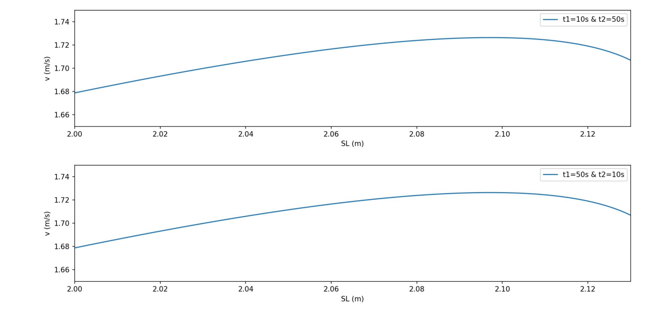
(9) $\begin{equation*}v(t) = SF_1 \cdot \Big( 1 - a \cdot (t - t_1)^2 \Big) \cdot SL_1 \cdot \Big( 1 - b \cdot (t - t_2)^2 \Big)\end{equation*}$

This approximated behavioral model aligns well with the relationships between swimming speed, stroke length, and stroke frequency reported by Keskinen & Komi (1988)¹⁹ and Pendergast (2006)²⁰. Comparable speed vs. stroke frequency and speed vs. stroke length curves are illustrated in Figure 2 and Figure 3.

Figure 2 | Swimming speed versus stroke frequency using the approximated model in Equation (9). The curves use representative elite freestyle values of SF₁=0.84 s⁻¹ and SL₁=2.14m. Varying the peak times t₁ (for stroke frequency) and t₂ (for stroke length) produces a quadratic relationship between speed and stroke frequency, consistent with findings reported by Keskinen & Komi (1988)¹⁹ and Pendergast (2006)²¹.

Figure 3 | Swimming speed versus stroke length using the approximated model in Equation (9). The curves are generated using representative elite freestyle values of SF₁=0.84 s⁻¹ and SL₁=2.14m. Varying the peak times t₁ (stroke frequency) and t₂ (stroke length) produces a quadratic relationship between speed and stroke length, consistent with observations reported by Keskinen & Komi (1988)¹⁹ and Pendergast (2006)²¹.

Furthermore, the parametric equation of $P_{\text{drag}}$ can be rewritten as,

(10) $\begin{equation*}\smallP_{\text{drag}}(t) = \frac{1}{2} \rho C_d A SF_1^3 \cdot SL_1^3 \cdot\left( 1 - \alpha \cdot (t - t_1)^2 \right)^3 \cdot\left( 1 - b \cdot (t - t_2)^2 \right)^3\end{equation*}$

Additionally, using the definition of stroke efficiency $\eta_{sk}$ , the total mechanical power $P_{sw}$ can be expressed in terms of $P_{\text{drag}}$ as,

(11) $\begin{equation*}P_{sw} = P_{\text{drag}} \cdot \frac{1}{\eta_{sk}}\end{equation*}$

Stroke efficiency generally decreases as stroke frequency increases, since higher frequencies are typically accompanied by shorter stroke lengths, larger intra cycle velocity fluctuations and greater energetic cost²². In this study, we approximate this relationship using a first order (linear) model, given by,

(12) $\begin{equation*}\eta_{sk}(SF) = \eta_1 \cdot \left( 1 - k \cdot \frac{SF - SF_1}{SF_1} \right)\end{equation*}$

Where, $\eta_1$ denotes the stroke efficiency at the baseline stroke frequency $SF_1$ , and k is the stroke frequency dependent coefficient for efficiency.

To combine the above two parametric equations of $P_{\text{sw}}$ and $\eta_{sk}$ in terms of time t, we can finally have:

(13) $\begin{equation*}\resizebox{\columnwidth}{}{$P_{sw} = C_1 \cdot\left( 1 - a (t - t_1)^2 \right)^3\cdot \left( 1 - b (t - t_2)^2 \right)^3\cdot \left( 1 - c (t - t_2)^2 \right) $}\end{equation*}$

Where

(14) $\begin{equation*}C_1 = \frac{1}{2} \rho C_d A SF_1^3 \cdot SL_1^3 \cdot \frac{1}{\eta_1}\end{equation*}$

and

$c = k \cdot a$

With the power being defined as a function of time, we can get the total mechanical work through the integral of power:

(15) $\begin{equation*}W_{\text{tot}} = \int_{0}^{t_f} P_{\text{sw}}(t, t_1, t_2)\, dt\end{equation*}$

Where, $t_f$ is the finish time of swimming. This is the work done over the course of the race, and is measured in J.

From the equation of $W_{\text{tot}}(t_f, t_1, t_2)$ , it is clear that the total mechanical work is a function of both the finish time $t_f$ and the stroke peak times for frequency and length, $t_1$ and $t_2$ .Through finding the minimum of $W_{\text{tot}}$ , we can find the relation between $t_f$ , $t_1$ and $t_2$ ,

(16) $\begin{equation*}\frac{\partial W_{\text{tot}}(t_f,t_1,t_2)}{\partial t_1} = 0,\qquad\frac{\partial W_{\text{tot}}(t_f,t_1,t_2)}{\partial t_2} = 0\end{equation*}$

Alternatively, we can find the minimum finish time $t_f$ for a given distance D through a similar approach, as shown below,

(17) $\begin{equation*}D = \int_{0}^{t_f} v(t, t_1, t_2)\, dt\end{equation*}$

Thus, $t_f$ is a function of D, $t_1$ and $t_2$ ,

(18) $\begin{equation*}t_f = t_f(D, t_1, t_2)\end{equation*}$

Through the optimization process of zero derivative of $t_f$ over $t_1$ and $t_2$ , we can find the minimum finish time $t_f$ with the optimal setting of $t_1$ and $t_2$ .

(19) $\begin{equation*}\frac{\partial t_f(D,t_1,t_2)}{\partial t_1} = 0,\qquad\frac{\partial t_f(D,t_1,t_2)}{\partial t_2} = 0\end{equation*}$

As a result, we can set this relation as an optimal stroke pattern. This pattern can also be found through numerical simulations.

Simulations and Results

An example of simulations on 100m freestyle swimming is exercised. The typical values of the parameters used in the simulations, as included in Equation (14), is illustrated in Table 1.

Parameter	Symbol	Value	Units	Source/Notes
Fluid density	ρ	1000	kg·m⁻³	Standard value for freshwater
Drag coefficient	C_d	0.9	–	Drag coefficient for freestyle swimming from Vilas-Boas (2010)²³
Frontal area	A	0.35	m²	Front area for a typical elite male swimmer from Toussaint (1988)²⁴
Stroke frequency (baseline)	SF₁	0.84	s⁻¹	Costa, M.J., et al. (2023)²⁵. Association between elite swimmers’ force production and 100m freestyle inter-lap pacing and kinematics.
Stroke length (baseline)	SL₁	2.14	m	Costa, M.J., et al. (2023)²⁵. Association between elite swimmers’ force production and 100m freestyle inter-lap pacing and kinematics.
Time dependent coefficient for stroke frequency	a	5.0e-5	s⁻²	Approximate +/- 10% variation over time, per data from Costa, M.J., et al. (2023)²⁵
Time dependent coefficient for stroke length	b	5.0e-5	s⁻²	Approximate +/- 10% variation over time, per data from Costa, M.J., et al. (2023)²⁵
Stroke efficiency at baseline SF	η₁	0.45	–	Propelling efficiency from Zamparo (2011)²⁶
Stroke frequency dependent coefficient for efficient	k	0.31	–	Derived from the relationship of the energy cost change over the stroke frequency change for male swimmer group study in Zamparo (2005)¹⁸
Event distance	D	100	m	Short distance simulation
Time step	Δt	0.01	s	Simulation time resolution
Simulation duration	t_f	solved	s	Set so ∫v(t)dt = D

Table 1| Model parameters and baseline values used in simulations for 100m freestyle

The stroke frequency dependent coefficient k for the efficiency η_sk can be obtained from the relationship of the energy cost change over the stroke frequency change, as reported in the previous study such as Zamparo (2005)¹⁸. The energy cost function C_SW is defined as follows:

(20) $\begin{equation*}C_{SW} = \frac{W_{tot}}{\eta_0} = \frac{W_d}{\eta_0 \cdot \eta_{sk}}\end{equation*}$

Where, $W_{tot}$ is the total mechanical work, as defined in Equation (15), $W_d$ is the work
to overcome hydrodynamic resistance, and $\eta_0$ is the total efficiency. When the variation of $\eta_{sk}$ with respect to stroke frequency is small, i.e. $k \ll 1$ as defined in Equation (12), the energy cost function can be approximated as,

(21) $\begin{equation*}C_{SW} \approx \frac{W_d}{\eta_0 \cdot \eta_1} \cdot \left( 1 + k \cdot \frac{SF - SF_1}{SF_1} \right)\end{equation*}$

The empirical data used to derive the coefficient k are extracted from the male swimmer group study in Zamparo (2005)¹⁸, as summarized in Table 2. A simple least squares linear fit was applied to estimate the first order dependence of energy cost on stroke frequency, as shown in Figure 4. Incorporating this first order relationship into Equation (21), the coefficient k can be computed as,

(22) $\begin{equation*}\frac{k}{1-k} \cdot \frac{1}{SF_1} = 0.53158\end{equation*}$

For the baseline stroke frequency of $SF_1 = 0.84~\text{s}^{-1}$ , the resulting calculated value of $k$ is 0.31.

Condition	Stroke Frequency SF (s^-1)	Energy Cost Function C_SW(KJm^-1)
Swimmer#1 (before the 2km trail)	0.627	0.89
Swimmer#2 (before the 2km trail)	0.665	1.10
Swimmer#3 (before the 2km trail)	0.705	1.31
Swimmer#1 (after the 2km trail)	0.645	1.05
Swimmer#2 (after the 2km trail)	0.675	1.08
Swimmer#3 (after the 2km trail)	0.725	1.27

Table 2| Energy cost function change over stroke frequency. Data is extracted from the male group study in Zamparo (2005)¹⁸

Figure 4 | Energy cost function versus stroke frequency. Data are extracted from the male swimmer group in Zamparo (2005)¹⁸. A least squares linear fit is applied to approximate the first order dependence of energy cost on stroke frequency.

Simulation results based on the parameters in Table 1 and three combinations of stroke frequency peak time t₁ and stroke length peak time t₂ are presented in Figure 5. The top panel shows stroke frequency trajectories for early (t₁=10s), mid (t₁=30s) and late (t₁=50s) peaking. The middle panel illustrates stroke length trajectories for early (t₂=10s), mid (t₂=30s) and late (t₂=50s) peaking. The bottom panel demonstrates that when both SF and SL peak at mid race (t₁=30s, t₂=30s), the resulting swimming speed v(t) is consistently higher than in the two offset peak conditions (t₁=10s, t₂=50s and t₁=50s, t₂=10s).

Figure 5 | Simulation results of stroke frequency (SF), stroke length (SL) and swimming speed (v) under different stroke pattern configurations. Three peak time combinations are shown: early SF and late SL (blue, t₁=10s & t₂=50s), late SF and early SL (green, t₁=30s & t₂=30s), and both variables peaking at mid race (orange, t₁=50s & t₂=10s). The top panel shows SF trajectories, the middle panel shows SL trajectories, and the bottom panel shows the resulting swimming speeds. The mid race peaking configuration produces the highest overall speed.

By varying t₁ and t₂, different stroke frequency and stroke length trajectories can be generated for the same swimmer, whose characteristics are specified in Table 1. Corresponding projections of finish time for a 100m freestyle swim, along with total mechanical work, are shown in Figure 6. Under identical peak values of stroke frequency and stroke length, the fastest finish time occurs when both variables peak at t₁ = t₂ = 30s; this configuration also results in the highest total mechanical energy expenditure. For more balanced performance, swimmers may instead adopt stroke patterns in which the peak times of stroke frequency and stroke length are offset, thereby reducing energy consumption while still maintaining competitive speed.

Figure 6 | Projected finish time (left) and total mechanical work (right) for a 100m freestyle swim, using the swimmer characteristics listed in Table 1. The left panel displays finish times across different combinations of stroke frequency peak time t₁ and stroke length peak time t₂. The fastest performance occurs when both t₁ and t₂ are set to 30s; however, as shown in the right panel, this configuration also yields the highest total mechanical work.

Various figure of merits (FoM) have been proposed to balance swimming speed and energy cost¹⁸^‘²⁷. One of the most widely used formulations, which assigns equal weight to both performance measures, is defined as follows,

(23) $\begin{equation*}\mathrm{FoM} = \frac{v}{C_{\mathrm{SW}}}\end{equation*}$

In this study, overall speed is computed as swimming distance divided by finish time, and total energy cost is represented by the total mechanical work. After normalizing these quantities relative to the world record finish time, the FoM can be expressed as,

(24) $\begin{equation*}\mathrm{FoM} = \frac{t_{\mathrm{world\,record}}}{t_{\mathrm{finish}}}\cdot \frac{1~\mathrm{kJ}}{W_{\mathrm{tot}}}\end{equation*}$

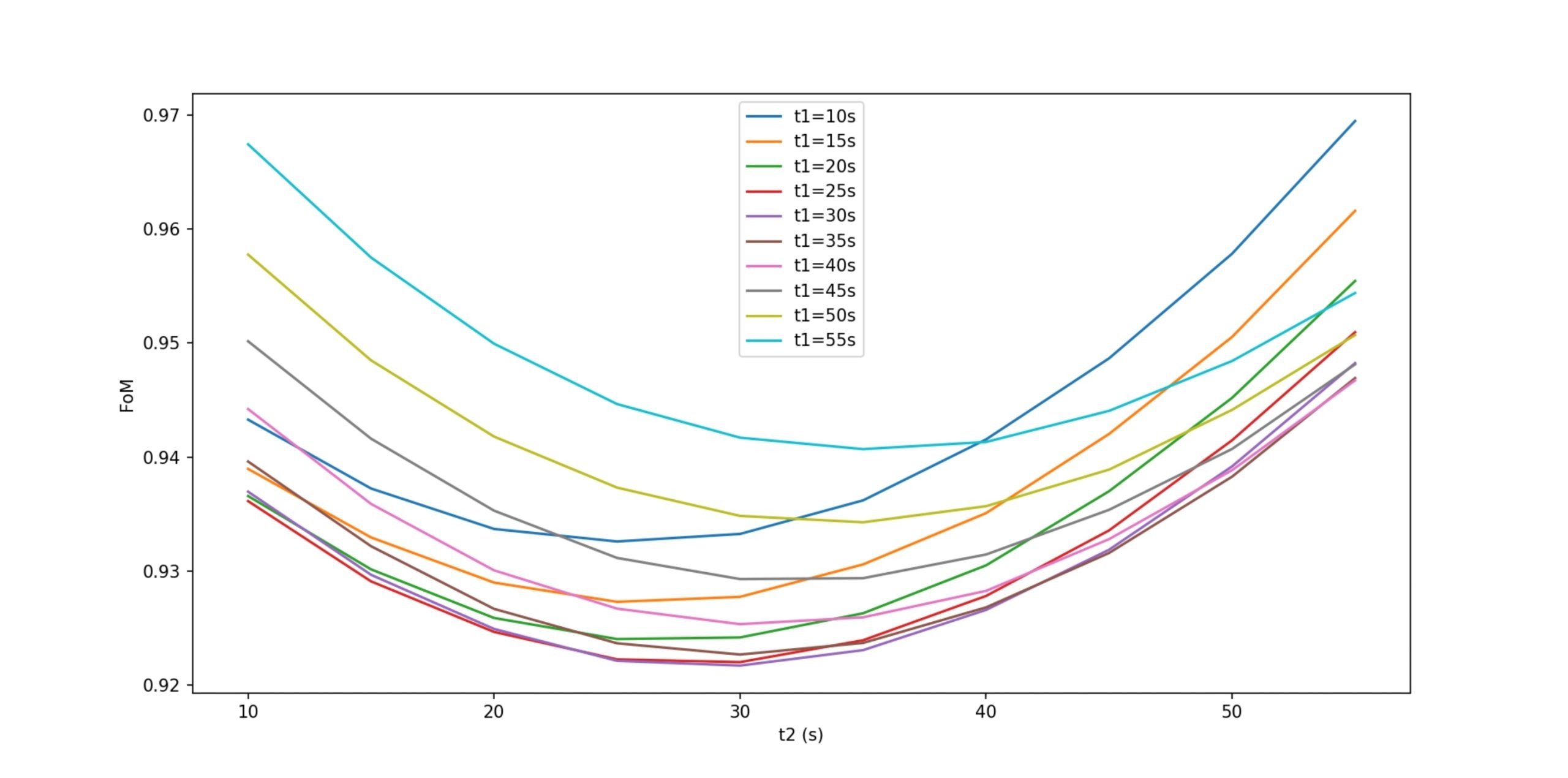
Where, $t_{\mathrm{world\,record}}$ is the world record finish time, (e.g., 46.4s for the 100m freestyle by Zhanle Pan at the 2024 Summer Olympics on 31 July 2024), $t_{\mathrm{finish}}$ is the swimmer’s projected finish time and $W_{\mathrm{tot}}$ is the total mechanical work for the swim. Using the simulated values of $t_{\mathrm{finish}}$ and $W_{\mathrm{tot}}$ from Figure 6, the resulting FoM across different stroke pattern combinations ( $t_1$ , $t_2$ ) is shown in Figure 7. Although synchronizing the peaks of stroke frequency and stroke length at mid race yields the highest overall speed, swimmers seeking a more balanced tradeoff between speed and energy expenditure may benefit from offsetting the peak times of these two variables.

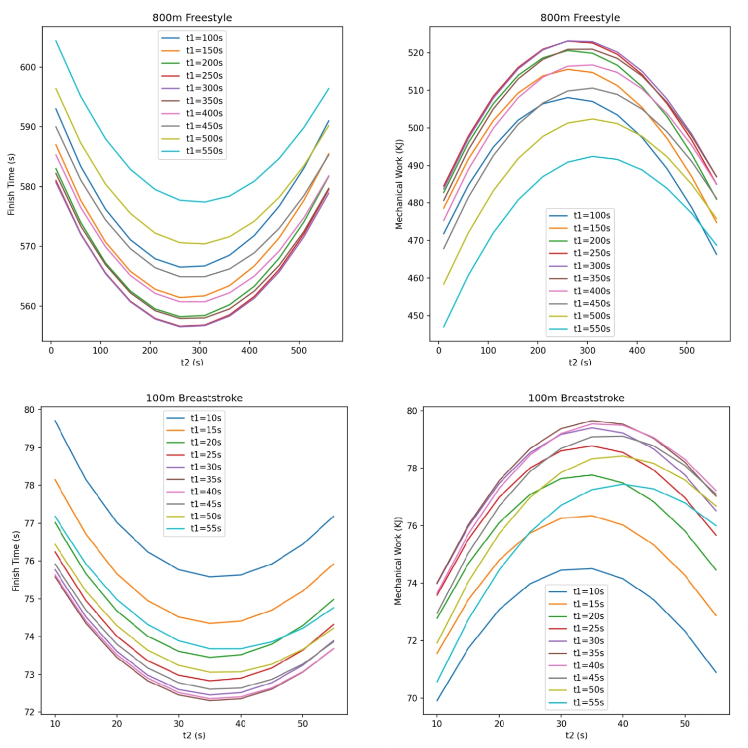
Figure 7 | Simulated figure of merit (FoM) incorporating both speed and total mechanical work. Comparable FoM formulations, balancing speed and energy cost, have been used in prior studies¹⁸^‘²⁷. While synchronizing the peak times of stroke frequency (t₁) and stroke length (t₂) at mid race (e.g., 30s) produces the fastest finish time, swimmers may achieve a higher overall FoM by offsetting these peak times to better balance speed and energy expenditure.

We applied the same modeling framework and simulation procedure to additional events, including the 800m freestyle and the 100m breaststroke, using the parameters summarized in Table 3. References directly supporting or used to derive these parameters are provided within the table. Simulations were conducted to identify the optimal stroke frequency and stroke length patterns for minimizing finish time or total mechanical work, as illustrated in Figure 8. Consistent with the 100m freestyle analysis, results for both the 800m freestyle and 100m breaststroke indicate that the fastest performances occur when stroke frequency and stroke length peak near the middle of the race; however, this configuration also produces the highest total mechanical work. Correspondingly, the figures of merit (FoMs) shown in Figure 9 confirm that offsetting the peak times of stroke frequency and stroke length yields more balanced performance, with improved FoM values for both events.

Parameter	Symbol	Units	Short Distance Freestyle	Long Distance Freestyle	Short Distance Breaststroke
Fluid density	ρ	kg·m⁻³	1000	1000	1000
Drag coefficient	C_d	–	0.90²³	0.90²³	1.10²³
Frontal area	A	m²	0.35²⁴	0.35²⁴	0.45²⁸
Stroke frequency (baseline)	SF₁	s⁻¹	0.84²⁵	0.72⁵	0.85³^‘⁴
Stroke length (baseline)	SL₁	m	2.14²⁵	2.05⁵	1.70³^‘⁴
Time dependent coefficient for stroke frequency	a	s⁻²	5.0e-5²⁵	5.0e-7²⁵	5.0e-5²⁵
Time dependent coefficient for stroke length	b	s⁻²	5.0e-5²⁵	5.0e-7²⁵	5.0e-5²⁵
Stroke efficiency at baseline SF	η₁	–	0.45²⁷	0.5²⁷	0.4²⁷
Stroke frequency dependent coefficient for efficient	k	–	0.31²⁹	0.2²⁹	0.35²⁹
Event distance	D	m	100	800	100
Time step	Δt	s	0.01	0.1	0.01

Table 3 | Model parameters used in simulations for short distance and long distance freestyle and short distance breaststroke

Figure 8 | Simulated finish time and total mechanical work for an 800m freestyle swim and a 100m breaststroke swim, using the swimmer characteristics defined in Table 3. The upper two panels correspond to the 800m freestyle simulations, while the lower two panels correspond to the 100m breaststroke simulations. The left panels show finish times across combinations of stroke frequency peak time t₁ and stroke length peak time t₂ , and the right panels show the corresponding total mechanical work. For both events, the shortest finish times occur when t₁ and t₂ peak near mid race, around 250s for the 800m freestyle and around 35s for the 100m breaststroke. However, as indicated in the right panels, these configurations also require the greatest total mechanical work.

Figure 9 | Figure of merit (FoM) simulations for an 800m freestyle swim and a 100m breaststroke swim. In both events, synchronizing the peak times of stroke frequency (t₁) and stroke length (t₂ ) at mid race yields the fastest finish times. However, offsetting these peak times results in higher overall FoM values, indicating a more favorable balance between speed and total mechanical energy expenditure.

Conclusion

Optimizing swimming performance, especially with respect to speed, requires careful planning of stroke patterns. By analyzing drag forces, propulsion mechanics, and the interaction between stroke rate and stroke length, it becomes possible to identify strategies that enable swimmers to maximize their speed in the water.

In this paper, we introduced an equation based model for analyzing swimming stroke patterns and developed a systematic framework for simulating and evaluating different stroke configurations. By examining the interplay between stroke rate and stroke length, swimmers can identify combinations that yield either maximal speed or improved efficiency, depending on performance goals.

Numerical simulations across varying parameter conditions demonstrate how the peak timing of stroke frequency (SF) and stroke length (SL) influences both energy expenditure and finishing time. The results show that when SF and SL peak simultaneously at mid race, swimmers achieve substantially lower finish times. However, this approach requires considerably more energy, up to 25% more than offset peak patterns. This tradeoff highlights the fundamental tension between optimizing for speed and optimizing for energy economy: short distance events favor the former, whereas middle and long distance events depend more heavily on the latter.

These findings also carry practical implications for training. In short distance events, athletes should develop the ability to maintain longer stroke lengths at high stroke frequencies, while in middle and long distance events, greater emphasis should be placed on movement economy and efficient energy distribution to sustain performance over time. Additionally, modern wearable monitoring technologies provide real time feedback on stroke parameters, enabling swimmers to approach the theoretically optimal patterns during both training and competition and facilitating data driven refinement of technique.

Nevertheless, this study has several limitations. The assumption that stroke frequency and stroke length trajectories follow quadratic profiles may not fully capture real world variability; the drag coefficient and frontal area were treated as constants, despite their dynamic dependence on speed and body position; and the absence of experimental validation limits the precision and generalizability of the model’s predictions. Future work that incorporates more empirical swimmer data into the modeling framework would enhance both its reliability and practical applicability.

Appendix

Table 4 Simulation codes in Python for finish time over stroke frequency and stroke length
#Simulation code for swimming stroke optimization.
import numpy as np
import matplotlib.pyplot as plt
import array as arr
import math

# Define constants
rho = 1000  # Water density (kg/m^3)
mu = 0.001  # Dynamic viscosity of water (Pa*s)
swimmer_mass = 70  # Swimmer's mass (kg)
A_hand = 0.02  # Area of hand (m^2)
A_body = 0.35  # Front area for a typical elite male swimmer 0.35 for freestyle from Toussaint (1988), 0.45 for breastroke from from Gatta (2014)
C_D_hand = 1.2  # Drag coefficient for the hand
C_D_body = 0.9  # Drag coefficient for front crawl from Vilas-Boas (2010)
C_L_hand = 0.8  # Lift coefficient for the hand
v_swimmer = 2.0  # Swimmer's velocity (m/s)
v_rel_hand = 5  # Relative velocity of hand to water (m/s)
angle_hand = 30  # Angle of attack for the hand (degrees)

SF1 = 0.84 #max stroke frequency, 0.84 for 100m freestyle, 0.85 for 100m breadstroke, 0.72 for 800m freestyle
SL1 =  2.14 #max stroke length, 2.14 for 100m freestyle, 1.70 for 100m breadstroke, 2.05 for 800m freestyle
eta0 = 0.45 #Propelling efficiency at baseline SF, from Zamparo(2011)

a_SF = 0.00005 # 2nd order coefficient for stroke frequency over time, 5E-5 for 100m freestyle and breadstroke, 5E-7 for 800m freestyle 
b_SL = 0.00005 # 2nd order coefficient for stroke length over time, 5E-5 for 100m freestyle and breadstroke, 5E-7 for 800m freestyle

# efficiency coefficient, derived from the relationship of the energy cost change
#over the stroke frequency change for male swimmer group study in Zamparo (2005)
k_eta = 0.31 # 0.31 for 100m freestyle, 0.35 for 100m breaststroke, 0.2 for 800m freestyle

dt = 0.01  # Time step (s)
L = 100.0 #race distance (m)

t_max = 1000*L/100 #max time for different distance
SF_min = 0.3 # min stroke frequency
SL_min = 0.5 # min stroke length
eta_min = 0.1 # min stroke effeciency

D = 0.0
t = 0.0
W = 0.0
v = 0.0



# Helper function to calculate force components
def calc_drag_force(C_D, A, v_rel):
    return 0.5 * C_D * rho * A * v_rel**2

def calc_lift_force(C_L, A, v_rel, angle):
    angle_rad = np.radians(angle)
    return 0.5 * C_L * rho * A * v_rel**2 * np.sin(angle_rad)



# Calculate drag and lift forces on the hand
F_drag_hand = calc_drag_force(C_D_hand, A_hand, v_rel_hand)
F_lift_hand = calc_lift_force(C_L_hand, A_hand, v_rel_hand, angle_hand)

# Calculate total propulsion force from the hand (assuming lift is effective forward force)
F_prop_hand =  F_drag_hand - F_lift_hand

def SF(t, t1): # (t^-1)
   return max(SF1 * (1 - a_SF * (t - t1)**2), SF_min)

def SL(t, t2): # (m)
   return max(SL1 * (1 - b_SL * (t - t2)**2), SL_min)
def eta(sf):
   return max(eta0*(1-k_eta*(sf-SF1)/SF1),eta_min)

t12_array=np.array([
    [10, 50],
    [30, 30],
    [50, 10]])
t=0
D1=0
t1=0
t2=0
d_t1=10
d_t2=10

#plot SF and SL
num_t12=t12_array.shape[0]

i=0
while(i<num_t12):
    
    t1=t12_array[i,0]
    t2=t12_array[i,1]


    xs1 = arr.array('f', [])
    ys1 = arr.array('f', [])
    zs1 = arr.array('f', [])
    vs1 = arr.array('f', [])
    es1 = arr.array('f', [])

    t=0
    D1=0

    while(D1<L and t < t_max):
       t = t + dt
       sf = SF(t,t1)
       sl = SL(t,t2)
       v1 = sf * sl 
       F_d1 = 0.5 * rho * v1**2 * C_D_body * A_body
       P1 = F_d1 * v1
       Ptotal_t11 = 1 / (1 - eta(sf)) * P1
       D1 = D1 + v1 * dt
       xs1.append(t)
       ys1.append(sf)
       zs1.append(sl)
       es1.append(eta(sf))
       vs1.append(v1)

    #figue
    plt.figure(1)
    plt.subplot(3,1,1)
    plt.plot(xs1,ys1,label=f't1={t1}s & t2={t2}s')
    plt.ylabel('SF (1/s)')
    plt.xlabel('t (s)')
    plt.legend()

    plt.subplot(3,1,2)
plt.plot(xs1,zs1,label=f't1={t1}s & t2={t2}s')
    plt.ylabel('SL (m)')
    plt.xlabel('t (s)')
    plt.legend()

    
    plt.subplot(3,1,3)
    plt.plot(xs1,vs1,label=f't1={t1}s & t2={t2}s')
    plt.ylabel('v (m/s)')
    plt.xlabel('t (s)')
    plt.legend()
    plt.tight_layout()
    
    #new figure
    plt.figure(2)
    plt.subplot(num_t12,1,i+1)
    plt.plot(ys1, vs1, label = f't1={t1}s & t2={t2}s')
    plt.xlabel('SF (1/s)')
    plt.ylabel('v (m/s)')
    plt.legend()
    plt.xlim(0.78, 0.83)
    plt.ylim(1.65, 1.75)
    plt.tight_layout()
 
    plt.figure(3)
    plt.subplot(num_t12,1,i+1)
    plt.plot(zs1, vs1, label = f't1={t1}s & t2={t2}s')
    plt.xlabel('SL (m)')
    plt.ylabel('v (m/s)')
    plt.legend()
    plt.xlim(2.0, 2.13)
    plt.ylim(1.65, 1.75)
    plt.tight_layout()

    i=i+1

plt.show()
plt.close("all")

exit()

Table 5 Simulation codes in Python for total mechanical work and figure of merit (FOM) over stroke frequency and stroke length
#Simulation code for swimming stroke optimization.
import numpy as np
import matplotlib.pyplot as plt
import array as arr
import math

# Define constants
rho = 1000  # Water density (kg/m^3)
mu = 0.001  # Dynamic viscosity of water (Pa*s)
swimmer_mass = 70  # Swimmer's mass (kg)
A_hand = 0.02  # Area of hand (m^2)
A_body = 0.35  # Front area for a typical elite male swimmer 0.35 for freestyle from Toussaint (1988), 0.45 for breastroke from from Gatta (2014)
C_D_hand = 1.2  # Drag coefficient for the hand
C_D_body = 0.9  # Drag coefficient for front crawl from Vilas-Boas (2010)
C_L_hand = 0.8  # Lift coefficient for the hand
v_swimmer = 2.0  # Swimmer's velocity (m/s)
v_rel_hand = 5  # Relative velocity of hand to water (m/s)
angle_hand = 30  # Angle of attack for the hand (degrees)

SF1 = 0.84 #max stroke frequency, 0.84 for 100m freestyle, 0.85 for 100m breadstroke, 0.72 for 800m freestyle
SL1 =  2.14 #max stroke length, 2.14 for 100m freestyle, 1.70 for 100m breadstroke, 2.05 for 800m freestyle
eta0 = 0.45 #Propelling efficiency at baseline SF, from Zamparo(2011)

a_SF = 0.00005 # 2nd order coefficient for stroke frequency over time, 5E-5 for 100m freestyle and breadstroke, 5E-7 for 800m freestyle 
b_SL = 0.00005 # 2nd order coefficient for stroke length over time, 5E-5 for 100m freestyle and breadstroke, 5E-7 for 800m freestyle

# efficiency coefficient, derived from the relationship of the energy cost change
#over the stroke frequency change for male swimmer group study in Zamparo (2005)
k_eta = 0.31 # 0.31 for 100m freestyle, 0.35 for 100m breaststroke, 0.2 for 800m freestyle

dt = 0.01  # Time step (s)
L = 100.0 #race distance (m)
t100F_record = 46.4 #Men’s world record: Pan Zhanle swam 46.40 s
#t100B_record = 56.88 #Men’s world record: long-course world record for the 100 m breaststroke is 56.88 seconds, set by Adam Peaty on 21 July 2019 in Gwangju
#t800F_record = 452.12 #Men’s world record: long-course 800 m freestyle world record is 7:32.12, set by Zhang Lin (China) on 29 July 2009

t_max = 1000*L/100 #max time for different distance
SF_min = 0.3 # min stroke frequency
SL_min = 0.5 # min stroke length
eta_min = 0.1 # min stroke effeciency

t1 = 10
dt1 = 0.1
D = 0.0
t = 0.0
W = 0.0
v = 0.0
vavg = 0.0
alpha = 0.1


# Helper function to calculate force components
def calc_drag_force(C_D, A, v_rel):
    return 0.5 * C_D * rho * A * v_rel**2

def calc_lift_force(C_L, A, v_rel, angle):
    angle_rad = np.radians(angle)
    return 0.5 * C_L * rho * A * v_rel**2 * np.sin(angle_rad)



# Calculate drag and lift forces on the hand
F_drag_hand = calc_drag_force(C_D_hand, A_hand, v_rel_hand)
F_lift_hand = calc_lift_force(C_L_hand, A_hand, v_rel_hand, angle_hand)

# Calculate total propulsion force from the hand (assuming lift is effective forward force)
F_prop_hand =  F_drag_hand - F_lift_hand

def SF(t, t1): # (t^-1)
   return max(SF1 * (1 - a_SF * (t - t1)**2), SF_min)

def SL(t, t2): # (m)
   return max(SL1 * (1 - b_SL * (t - t2)**2), SL_min)

def eta(sf):
   return max(eta0*(1-k_eta*(sf-SF1)/SF1),eta_min)

max_t1=60
max_t2=60

t=0
D1=0
t1=0
t2=0
d_t1=5
d_t2=5


t1=10

while(t1<max_t1):

    t2s = arr.array('f', [])
    tfinishs = arr.array('f', [])
    Ws = arr.array('f', [])
    FoMs = arr.array('f',[])
    
    t2=10
    
    while(t2<max_t2):

        t=0
        D1=0
        W=0

        while(D1<L and t < t_max):
           t = t + dt
           sf = SF(t,t1)
           sl = SL(t,t2)
           v1 = sf * sl 
           F_d1 = 0.5 * rho * v1**2 * C_D_body * A_body
           P1 = F_d1 * v1
           Ptotal = 1 / (1 - eta(sf)) * P1
           D1 = D1 + v1 * dt
           W = W + Ptotal * dt

        #Calculate FoM = vavg_normalized / Wtot_normalized 
        #FoM = 2*math.log(t)+1*math.log(W)
        FoM = (t100F_record/t) * 100000/W

        t2s.append(t2)
        tfinishs.append(t)
        Ws.append(W/1000)
        FoMs.append(FoM)

        t2=t2+d_t2

    #figue
    plt.figure(1)
    plt.subplot(1,2,1)
    plt.plot(t2s,tfinishs,label=f't1={t1}s')
    plt.ylabel('Finish Time (s)')
    plt.xlabel('t2 (s)')
    plt.legend()

    plt.figure(1)
    plt.subplot(1,2,2)
    plt.plot(t2s,Ws,label=f't1={t1}s')
    plt.ylabel('Mechanical Work (KJ)')
    plt.xlabel('t2 (s)')
    plt.legend()

    plt.tight_layout()

    plt.figure(2)
    plt.plot(t2s,FoMs, label=f't1={t1}s')
    plt.ylabel('FoM')
    plt.xlabel('t2 (s)')
    plt.legend()
    
    t1=t1+d_t1

plt.show()
plt.close("all")

exit()

References

Barbosa, T. M., Marinho, D. A., Costa, M. J., & Silva, A. J. Biomechanics of competitive swimming strokes. Biomechanics in Applications, 367–388. https://doi.org/10.5772/19553 (2011). [↩] [↩]
Barbosa, T. M., Costa, M. J., Marques, M. C., Silva, A. J., & Marinho, D. A. A model for active drag force exogenous variables in young swimmers. Journal of Human Sport and Exercise, 5(3), 379–388. https://doi.org/10.4100/jhse.2010.53.08 (2010). [↩] [↩]
Takagi, H., & Wilson, B. Vortex generation in breaststroke pullout technique. Journal of Swimming Research, 14, 15–21. (1999). [↩] [↩] [↩]
Seifert, L., Chollet, D., & Rouard, A. Interlimb coordination and phase characteristics in breaststroke. International Journal of Sports Medicine, 28(1), 68–73. (2007). [↩] [↩] [↩]
Morais, J. E., Sanders, R. H., Papic, C., Barbosa, T. M., & Marinho, D. A. The influence of the frontal surface area and swim velocity variation in front crawl active drag. Medicine & Science in Sports & Exercise, 52(11), 2357–2364. https://doi.org/10.1249/mss.0000000000002400 (2020). [↩] [↩] [↩] [↩] [↩]
Kolmogorov, S. V., & Duplishcheva, O. A. Active drag, useful mechanical power output and hydrodynamic force in different swimming strokes. Journal of Biomechanics, 25(3), 311–318. (1992). [↩]
Toussaint, H. M., & Beek, P. J. Biomechanics of competitive front crawl swimming. Sports Medicine, 32(12), 761–775. (2002). [↩] [↩]
Chollet, D., Chalies, S., & Chatard, J. C. Comparison of gliding and stroking phases in freestyle using time-distance variables. Journal of Human Movement Studies, 38(1), 35–49. (2000). [↩] [↩]
Stamm, A., James, D. A., & Thiel, D. V. Velocity profiling using inertial sensors for freestyle swimming. Sports Engineering, 16(1), 1–11. (2013). [↩]
Mooney, R., Corley, G., Godfrey, A., Quinlan, L. R., & OLaighin, G. Monitoring of swimming performance using inertial sensors: A systematic review. Sports Biomechanics, 15(2), 214–231. (2016). [↩]
Gatta, G., Cortesi, M., Fantozzi, S., & Zamparo, P. Planimetric frontal area in the four swimming strokes: Implications for drag, energetics and speed. Human Movement Science, 39, 41–54. https://doi.org/10.1016/j.humov.2014.06.010 (2014). [↩]
Garrett, A., & Kirkendall, D. Propulsion, drag, and stroke mechanics in human swimming. Exercise and Sport Sciences Reviews, 19(1), 125–156. (1991). [↩]
Winter, D. A. Biomechanics and Motor Control of Human Movement (4^th ed.). Wiley. (2009). [↩]
Collins, S. H., Ruina, A., Tedrake, R., & Wisse, M. Efficient bipedal robots based on passive-dynamic walkers. Science, 307(5712), 1082–1085. (2005). [↩]
Praagman, M., Chadwick, E. K., van der Helm, F. C., & Veeger, H. E. The relationship between two different mechanical cost functions and muscle oxygen consumption. Journal of Biomechanics, 39(4), 758–765. (2006). [↩]
Ernest W Maglischo. Swimming Fastest, Human Kinetics. (2003). [↩] [↩]
Barbosa, T. M., Bragada, J. A., Reis, V. M., Marinho, D. A., Carvalho, C., & Silva, A. J. Energetics and biomechanics as determining factors of swimming performance: Updating the state of the art. Journal of Science and Medicine in Sport, 13(2), 262–269. (2010). [↩]
Zamparo P., Bonifazi M., Faina M., Milan A., Sardella F., Schena F., Capelli C. Energy cost of swimming of elite long‑distance swimmers. European Journal of Applied Physiology, 94(5-6), 697-704. DOI:10.1007/s00421-005-1337-0. (2005). [↩] [↩] [↩] [↩] [↩] [↩] [↩] [↩]
Keskinen, K.L. & Komi, P.V. The stroking characteristics in four different exercises in freestyle swimming. Biomechanics XI-B, 839-843, Free University Press, Amsterdam. (1988). [↩] [↩] [↩]
Pendergast, D.R., Capelli, C., Craig, A.B., di Prampero, P.E., Minetti, A.E., Mollendorf, J., Termin, .I.I. & Zamparo, P. Biophysics in swimming. Biomechanics and Medicine in Swimming X, 185-189, Portuguese Journal of Sport Science, Porto. (2006). [↩]
Pendergast, D.R., Capelli, C., Craig, A.B., di Prampero, P.E., Minetti, A.E., Mollendorf, J., Termin, .I.I. & Zamparo, P. Biophysics in swimming. Biomechanics and Medicine in Swimming X, 185-189, Portuguese Journal of Sport Science, Porto. (2006). [↩] [↩]
Yanai, T. Stroke frequency in front crawl: Its mechanical link to the propelling efficiency. Journal of Biomechanics, 36(1), 53–62. (2003). [↩]
Vilas-Boas, J. P., Costa, L., Fernandes, R., Machado, L., & Fernandes, C. Determination of the drag coefficient during the first and second gliding positions of the breaststroke underwater stroke. Journal of Applied Biomechanics, 26(3), 324-331. (2010). [↩] [↩] [↩] [↩]
Toussaint, H. M., Beelen, A., Rodenburg, A., Sargeant, A. J., de Groot, G., Hollander, A. P., & van Ingen Schenau, G. J. Propelling efficiency of front-crawl swimming. Journal of Applied Physiology, 65(6), 2506-2512. doi:10.1152/jappl.1988.65.6.2506. (1988). [↩] [↩] [↩]
Costa MJ, Santos CC, Ferreira F, Arellano R,Vilas-Boas J.P and Fernandes RJ. Association between elite swimmers’ force production and 100 m front crawl inter-lap pacing and kinematics. Front. Sports Act. Living 5:1205800. doi:10.3389/fspor.2023.1205800. (2023). [↩] [↩] [↩] [↩] [↩] [↩] [↩] [↩] [↩] [↩] [↩] [↩]
Zamparo P., Capelli C., Pendergast D.R. Energetics of swimming: a historical perspective. European Journal of Applied Physiology, 111(3), 367-378. DOI:10.1007/s00421-010-1433-7. (2011). [↩]
Zamparo P., Cortesi M., Gatta G. The energy cost of swimming and its determinants. European Journal of Applied Physiology, 120(1), 41-66. DOI:10.1007/s00421-019-04270-y. (2020). [↩] [↩] [↩] [↩] [↩]
Gatta, G., Cortesi, M., Fantozzi, S., & Zamparo, P. Planimetric frontal area in the four swimming strokes: Implications for drag, energetics and speed. Human Movement Science, 39, 41–54. https://doi.org/10.1016/j.humov.2014.06.010 (2014). [↩]
Zamparo P., Bonifazi M., Faina M., Milan A., Sardella F., Schena F., Capelli C. Energy cost of swimming of elite long‑distance swimmers. European Journal of Applied Physiology, 94(5-6), 697-704. DOI:10.1007/s00421-005-1337-0. (2005). [↩] [↩] [↩]

Modeling for Optimizing the Patterns of Swimming Strokes

Abstract

Introduction