
Abstract
Ever since the first discovery of an exoplanet in the 1990s, there has been an abundance of exoplanet research and discovery as more bodies are being detected with better technology. The goal of the research was to develop a machine learning model that can predict whether an observation is a candidate for an exoplanet or not. It is important because discovering more exoplanets could lead to better research on exoplanets. Using python and python libraries, we created a model that would be able to predict whether an observation was a candidate for an exoplanet based on the characteristics of the exoplanet. The model was trained using data from the NASA exoplanet database with 9564 unique values. The final model was able to produce an accuracy of over 80% of classifying whether an observation was an exoplanet or not, while being able to analyze a large data set over a short period of time. With the inclusion of more characteristics or data points, the model could be further improved to be more accurate. However, even with just two input features, which were selected based on domain knowledge, it is possible for the model to be above 80% accurate. This is revealed through the feature importance plot created for the RandomForestClassifier model.
Introduction
Planets outside of the solar system are a great subject of study in astronomy, and have been studied intensely over the past few decades. The first ever exoplanet around a solar like star was discovered by Mayor and Queloz in 19951. Many missions, including the Kepler mission hunted for planets in the Milky Way Galaxy. The Kepler mission, a space based telescope observing in visible light, was launched in 2009 by NASA, and it was created to analyze and monitor planetary candidates that were earth-sized. Over a thousand confirmed candidates were found, hundreds of Earth-sized planetary candidates were discovered, and Earth-sized planets in the habitable zone were detected2. The mission was also NASA’s first exoplanet mission, and transits were used to monitor 100,000 main sequence stars over 3 and a half years. This mission showed that our galaxy contained billions of exoplanets, which could hold life3.
This information allows scientists to put into perspective the frequency of exoplanets in our galaxy, and the possibility of discovering an exoplanet that is habitable grows larger. Thus, the ever growing demand and field of discovering exoplanets can be further improved with help from machine learning, as machine learning provides a way to quickly sort through information and data in a way that humans are unable to. The application of machine learning can make the discovery and analysis of exoplanets much easier, quicker, and more cost-efficient. This information can then be put to use to discover life beyond Earth, discover more about our solar system.
An exoplanet candidate is one that is a likely planet discovered by a telescope but not yet proven to exist. The majority of exoplanet candidates are discovered through the “transit method”. In this case, the light from the star is temporarily obscured by a planet passing in front of it, in many cases only a small fraction (few parts in a thousand). The Kepler space telescope, and more recently, the Transiting Exoplanet Survey Satellite (TESS) are examples of space-based missions that used the transit technique, and led to thousands of exoplanet candidates. TESS data has been used to confirm long orbital period exoplanets, allowing for a more accurate database4. A confirmed exoplanet is one that is verified with two additional telescopes, and thus more observations are needed to determine whether an exoplanet is confirmed or not. Sometimes, the “signal-to-noise” ratio is very low, meaning that the light curve is has strong noise usually due to the faintness of the star. In these cases, other techniques are needed to confirm an exoplanet. For example, the radial velocity technique may be used after the initial discovery to confirm that the star is being gravitationally “wobbled” by a planet in the orbit. In order to do this manually, however, it would be more costly and time consuming. Therefore, in order to boost the efficiency of determining whether an observation can actually be a confirmed exoplanet, machine learning can be used. Artificial Intelligence has already been applied to inferring star rotation patterns through deep learning, showing the effectiveness of machine learning in handling large amounts of data5. Additionally, convolutional neural networks (CNNs) have been used to separate eclipsing binaries and false positives from planet candidates6. The problem we worked with was a supervised classification problem of developing a machine learning model that can predict whether an observation is a real candidate for an exoplanet. The machine learning model classified observations as either candidate, confirmed, or false positive. The numerical data from NASA’s database was collected through the Kepler mission. While similar studies mentioned above apply machine learning to astronomical data and may be more accurate, the methodology used in this study is simpler and much more efficient in how it works.
Dataset
The dataset used for this project is the NASA and Caltech exoplanet dataset. The data was collected from the Kepler mission which discovered thousands of planets in the solar system7. There are 9564 unique, numerical values gathered in the dataset. In order to characterize the dataset, several histograms and a scatterplot were plotted, which are shown in Figures 1 to 4.
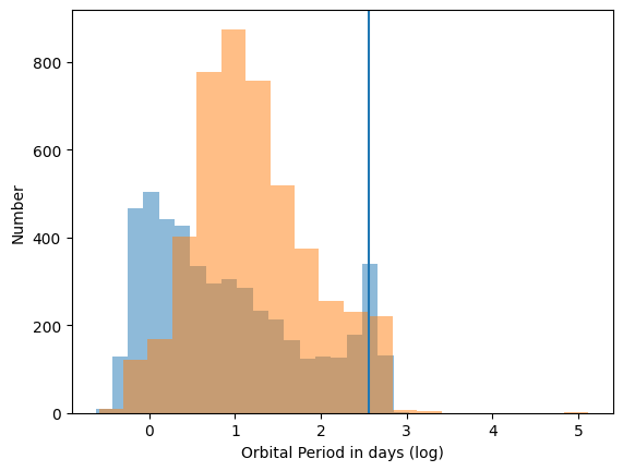
Figure 1. The blue is the distribution of false positives, and the orange of true planets. The blue line shows that a common period in the false positives is simply a year (365 days), which imprints onto the dataset.

Figure 2: The number of false positives increases with transit depth since false positives are dominated by brown dwarfs and low mass stars, which are larger and can block more stellar light. The difference in distributions here motivates the use of machine learning in this study, since previous assumptions may be biased towards larger transit depths, which are easier to detect.
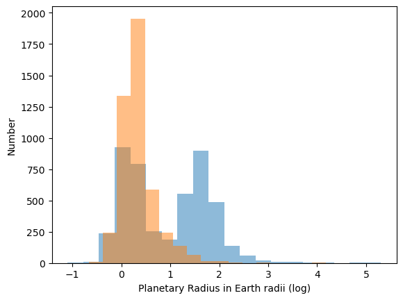
Figure 3: The bimodality of the false positive distribution can be explained by the large number of false positives in Figure 1 that have supposed year-long periods. This is also correlated to the large number of false positives in Figure 2 that show deep transits, which indicate large radii. Both of these are false and, if misinterpreted, would point to two very different planetary populations.

Figure 4: This scatter plot visualizes the relation between stellar temperature and planetary radius. No obvious trend is clear, except that the largest true planets tend to be located around hotter stars.
The 9564 objects were classified as either a ‘CONFIRMED’, ‘CANDIDATE’, or ‘FALSE POSITIVE’ exoplanet in the ‘koi_disposition’ column. The data set also provided characteristics of each entry, including orbital period, transit duration, and others. To preprocess the data, only certain columns pertaining to the research question were studied with the machine learning. The included columns are: koi_disposition: Exoplanet Archive Disposition, koi_period: Orbital Period [days], koi_time0bk: Transit Epoch [BKJD], koi_impact: Impact Parameter, koi_duration: Transit Duration [hrs], koi_depth: Transit Depth [ppm]. koi_prad: Planetary Radius [Earth radii], koi_teq: Equilibrium Temperature [K], koi_insol: Insolation Flux [Earth flux], koi_model_snr: Transit Signal-to-Noise, koi_steff: Stellar Effective Temperature [K], koi_slogg: Stellar Surface Gravity, koi_srad: Stellar Radius [Solar radii], koi_kepmag: Kepler-band [mag]. Entries without data were filled in with the average value of that column. This was chosen as to not throw out many rows of useful data, and the Gaussian trend of many features justified this assumption. The effectiveness of filling in empty values could be enhanced with incorporating KNN imputation. These features were chosen because of their ability to describe the planetary orbit and parameters (e.g. orbital period, transit epoch, transit duration, planetary radius), as well as features that concern the modeling of the transit itself (e.g. signal to noise, transit depth, impact parameter). Additionally, some features are related to the star itself, which has been underutilized in planetary detection and may prove to be ultimately just as useful as planetary parameters (e.g. stellar temperature, surface gravity, radius). The column ‘koi_disposition’ had its values replaced by either 1 or 0- where 1 represents a ‘CONFIRMED’ or ‘CANDIDATE’ classification, and 0 represents a ‘FALSE POSITIVE’ classification. This was done to make model development easier. Only two categories were used since the goal of this project is to use machine learning to simplify the selection of true planet candidates, and making three classes would generate an additional class of uncertain planet labels. The three class problem was also avoided due to the problem of imbalance that would result due to the low number of ‘CONFIRMED’ exoplanets. When testing the data, the train-test-split was 80% to 20%, where 80% of the data was used as training data, and 20% of the data was used as testing data. Training data is the subset of the data that generates the weights for the machine learning model, and the test data is the subset of the data that that model is tested on to assess the performance of the model.
Methodology/Models
| Feature Name | Description |
| ‘koi_disposition’ | Exoplanet Archive Disposition |
| ‘koi_period’ | Orbital Period [days] |
| ‘koi_impact’ | Impact Parameter |
| ‘koi_duration’ | Transit Duration [hrs] |
| ‘koi_depth’ | Transit Depth [ppm] |
| ‘koi_prad’ | Planetary Radius [Earth radii] |
| ‘koi_teq’ | Equilibrium Temperature [K] |
| ‘koi_model_snr’ | Transit Signal-to-Noise |
| ‘koi_steff’ | Stellar Effective Temperature [K] |
| ‘koi_srad’ | Stellar Radius [Solar radii] |
| ‘koi_slogg’ | Stellar Surface Gravity |
Table 1: Features/Columns included in data analysis
Important categories from the NASA dataset were imported into a dataframe, shown in Table 1. As mentioned above, columns that contained no values had the entries with no values filled with the average of the rest of the values in that column. Relevant columns included in model development were discussed in the dataset section. ‘CONFIRMED’ and ‘CANDIDATE’ for the ‘koi_disposition’ column, which was the column being analyzed, were replaced with 1, while ‘FALSE POSITIVE’ in ‘koi_disposition’ was replaced with 0 to make analysis easier. The columns were all read into a dataframe. Data preprocessing was completed with these steps, and the data was visualized using histograms and scatter plots. The first histogram shown has orbital period in days (log) on the x-axis. The second plot has transit depth in ppm (log) on the x-axis, the third plot has planetary radius in Earth radii (log) on the x-axis. All histograms have the number of either category on the y-axis. The false positives are colored in blue, and the confirmed and candidates are colored in orange. The scatterplot which is shown has koi_prad on the x-axis, and koi_steff on the y-axis, which are the planetary radius and the stellar effective temperature respectively. The hue is ‘koi_disposition’ and the observations labeled with a ‘0’ are blue and the ones labeled with a ‘1’ are orange. Using train_test_split, the model was developed with a test_size of 0.2. A single random seed was used and a single run was used, but the outputs remained consistent when experimenting with different random seeds. Machine learning models, such as Ridge Classifier, Logistic Regression, Random Forest Classifier, and Decision Tree Classifier were used to find the accuracy, precision, recall, and F1 scores of the model. The choice of Random Forest Classifier and Logistic Regression is justified as Random Forest is a local classifier and Logistic Regression is a global classifier. Models like SVM were avoided because of the inability of linear decision bounds to explain the data. Random Forest Classifier was also used due to its ability to highlight feature importance, as shown in Figure 5. Scikit-learn’s Mean Decrease Impurity (MDI) was used to determine feature importance for Random Forest Classifier, and the resulting plot is shown in Figure 5. Cross validation techniques were avoided as the choice of different random seeds yielded consistent results.
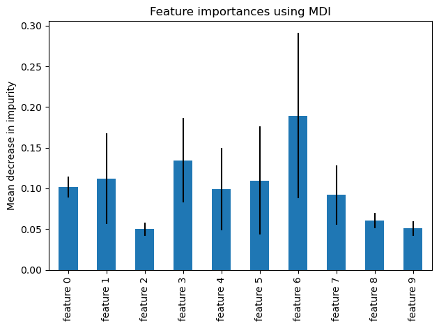
Figure 5: Feature 6 is clearly shown to be the most important, with Features 2, 8, and 9 all being the least important for prediction. The large error bars are likely inflated from the small number of trials run in the randomization process to generate them, but detailed estimates are beyond the scope of this work.
The feature that was determined to contribute the most to accuracy was feature 6, ‘log_koi_prad,’ followed by features 3 and 1, ‘log_koi_period’ and ‘koi_teq’ respectfully. The next most impactful features based on MDI are ‘log_koi_depth’ and ‘koi_duration,’ which are features 5 and 0 respectively. The combination of features that were found to have the greatest accuracy on Random Forest Classifier were ‘log_koi_period’ and ‘log_koi_prad.’ To increase the accuracy of the model, hyperparameter tuning was used, and grid search was used to pick the best value of hyperparameter.
| Models | Models | Models | Models | |
|---|---|---|---|---|
| Model Metrics | Ridge Classifier | Logistic Regression | Random Forest Classifier | Decision Tree Classifier |
| Accuracy (%) | 76.86 | 77.68 | 84.98 | 81.93 |
| Candidate Exoplanet Class Precision | 0.70981 | 0.73604 | 0.83640 | 0.79568 |
| Candidate Exoplanet Class Recall | 0.92184 | 0.87473 | 0.87580 | 0.86724 |
| Candidate Exoplanet Class F1 | 0.80205 | 0.79941 | 0.85565 | 0.82992 |
| Not Exoplanet Class Precision | 0.88301 | 0.83906 | 0.86496 | 0.84860 |
| Not Exoplanet Class Recall | 0.61019 | 0.67553 | 0.82281 | 0.76966 |
| Not Exoplanet Class F1 | 0.72168 | 0.74847 | 0.84336 | 0.80720 |
In order to hyperparameter tune RidgeClassifer, the alpha parameter was modified. The alpha parameter determines how much regularization is applied, and larger values discourage overfitting more than smaller values. Larger values of alpha shrink coefficients more, and larger coefficients are penalized. With the optimal alpha value of 0.4, the model metrics of RidgeClassifier are as follows: RidgeClassifier: 76.86%. Candidate exoplanet class: precision=0.7098103874690849, recall=0.9218415417558886, F1=0.8020493712156496. Not exoplanet class: precision=0.8830128205128205, recall=0.6101882613510521, F1=0.7216764898493778. The confusion matrix is shown in Figure 6 and the hyperparameter tuning graph is Figure 7.
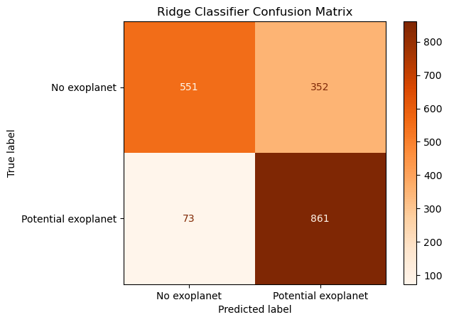
Figure 6: The confusion matrix shows that on average, the classifier is accurate, with the majority of labels being true positives and true negatives. The diagonal matrix elements are the smallest values, showing that this is justified. The potential exoplanet label also includes true exoplanets, demonstrating that both true and potential exoplanets can be grouped into the same category
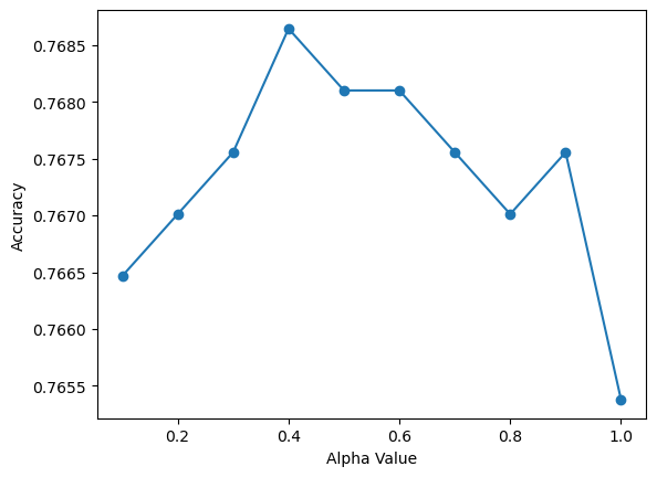
Figure 7: The lack of improvement of accuracy as a function of alpha is to be expected, mostly due to the small number of features used in the model and reliability based on the simplest model.
Precision is defined as true positives over all positives, and recall is true positives over the sum of true positives and false negatives, and the F1 score is the harmonic mean of precision and recall. The Confusion Matrix was plotted and is included below. For Logistic Regression, no hyperparameter tuning was used and the final model metrics are Logistic Regression Model Accuracy: 77.68%. Candidate exoplanet class: precision=0.7360360360360361, recall=0.8747323340471093, F1=0.7994129158512722. Not exoplanet class: precision=0.8390646492434664, recall=0.6755260243632336, F1=0.7484662576687118. The confusion matrix is also plotted in Figure 8.

Figure 8: Confusion matrix of Logistic Regression.
For RandomForestClassifier, the max_depth was tuned. The max depth of RandomForestClassifier controls how long the path is from the root node to the leaf node. The max_depth which produced the best accuracy was found to be 15. In the graph below, the max_depth is plotted on the x-axis and the accuracy is plotted on the y axis. With this max_depth, the model metrics are Random Forest Classifier Model Accuracy: 84.98%. Candidate exoplanet class: precision=0.83640081799591, recall=0.8758029978586723, F1=0.8556485355648535. Not exoplanet class: precision=0.8649592549476135, recall=0.82281284606866, F1=0.8433598183881953. The confusion matrix is plotted as Figure 9 and the hyperparameter tuning is shown in Figure 10.
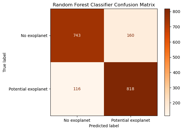
Figure 9: Confusion matrix of Random Forest Classifier.

Figure 10: Hyperparameter tuning of Random Forest Classifier.
Lastly, for DecisionTreeClassifier, the max_depth was also tuned, similar to RandomForestClassifier. The optimal max_depth was tuned to be 6, which was the value that provided the highest accuracy. The graph shows the plots of the accuracy of the model when the max_depth is between 1 and 15. The model metrics are Decision Tree Classifier Model Accuracy: 81.93%. Candidate exoplanet class: precision=0.7956777996070727, recall=0.867237687366167, F1=0.8299180327868851. Not exoplanet class: precision=0.8485958485958486, recall=0.769656699889258, F1=0.8072009291521486. The confusion matrix is Figure 11 and the hyperparameter tuning is Figure 12.

Figure 11: Confusion Matrix of Decision Tree Classifier.
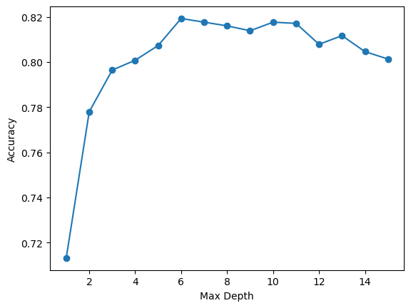
Figure 12: Hyperparameter tuning of Decision Tree Classifier.
Discussion
After hyperparameter tuning, the model that provided the best accuracy was RandomForest, with an accuracy of 84.98%. A possible explanation could be RandomForest’s effectiveness when analyzing large datasets, being less sensitive to outliers, and overcoming overfitting. Random forest classification is also found to achieve better results than decision trees most of the time, as it contains all the benefits of decision trees, along with being able to use multiple trees to prevent overfitting. Random Forest Classifier also uses bagging, which provides generalization and decreases bias8. However, even after hyperparameter tuning, the model is still not fully able to correctly categorize potential exoplanets. With RandomForest, the precision of finding a candidate exoplanet and not an exoplanet were pretty similar. In other models, however, such as Logistic Regression and Ridge Classifier, the model was much higher precision in the not exoplanet class, meaning the model is not as accurately able to determine potential exoplanets, and instead classifies them as not exoplanets. A logistic regression model could suffer from the problem of outliers when they go undetected9. Logistic regression could also have issues in having a poor fit10,11. If problematic points/outliers are not accounted for, where the observed value and the model value are not in agreement, this could have a great impact on model results12. Even without the benefit of having a very high accuracy, the models can be quickly run and data can be quickly analyzed. RandomForest was able to give results in 3.5s with 9564 data points, each with 6 features, corresponding with 57384 data points. Therefore, the models can be quickly used to quickly gather information, and are beneficial in that regard.
Conclusion
In this study, supervised learning was conducted on the NASA Exoplanet dataset, and the accuracy, precision, F1 score, and recall score were calculated for four models: Logistic Regression, Decision Tree Classifier, Ridge Classifier, and Random Forest Classifier. All models had at least a 75% accuracy rate. The model that performed the best was the Random Forest Model. With the inclusion of more data, the accuracy rate could increase. Synthetic data could increase model performance, and it is possible that the model could have a much higher accuracy. Additionally, it would be beneficial to explore other models, including incorporating deep learning architectures such as convolutional neural networks or ensemble methods such as gradient boosting. This work demonstrates the incredible efficiency in classifying exoplanets that would take a much longer time to classify by hand. The study of exoplanets has great potential to be a field of many discoveries and increasing the knowledge of possible other habitable worlds. By incorporating follow-up data from other telescopes, the classification accuracy of this model can be improved and further investigated. Moreover, all of the data and associated models presented in this paper can be made available upon request of citizen scientists.
Acknowledgments
I would like to thank my mentor, Tony Rodriguez, and my parents for supporting me through this process.
References
- M. Mayor, D. Queloz. A Jupiter-mass companion to a solar-type star. Nature. 378, 355–359 (1995). [↩]
- W. Borucki. KEPLER Mission: development and overview. https://iopscience.iop.org/article/10.1088/0034-4885/79/3/036901/meta (2016). [↩]
- S. Carney. Kepler / K2. https://science.nasa.gov/mission/kepler/ (2025). [↩]
- D. Bass, D. Fabrycky. Validating the orbital periods of the coolest Tess exoplanet candidates. https://arxiv.org/abs/2411.17640 (2024). [↩]
- Z. R. Claytor, J. L. van Saders, J. Llama, P. Sadowski, B. Quach, E. A. Avallone. Recovery of TESS Stellar Rotation Periods Using Deep Learning https://arxiv.org/pdf/2104.14566 (2021). [↩]
- V. T. Poleo, N. Eisner, D. W. Hogg. NotPlaNET: Removing false positives from planet hunters tess with machine learning. https://arxiv.org/abs/2405.18278 (2024). [↩]
- Möbius. NASA Exoplanet Dataset https://www.kaggle.com/datasets/arashnic/exoplanets/data (2024). [↩]
- J. Ali, R. Khan, N. Ahmad, I. Maqsood. Random Forests and Decision Trees. https://www.uetpeshawar.edu.pk/TRP-G/Dr.Nasir-Ahmad-TRP/Journals/2012/Random%20Forests%20and%20Decision%20Trees.pdf (2012). [↩]
- D. E. Jennings. Outliers and Residual Distributions in Logistic Regression. Journal of the American Statistical Association, 81, 987–990. https://doi.org/10.1080/01621459.1986.10478362 (1986). [↩]
- T. P. Ryan. Some issues in logistic regression. Communications in Statistics – Theory and Methods, 29, 2019–2032. https://doi.org/10.1080/03610920008832593 (2000). [↩]
- T. G. Nick, K. M. Campbell. Logistic Regression. Topics in Biostatistics, 404, 273–301. https://doi.org/10.1007/978-1-59745-530-5_14 (2007). [↩]
- M. P. LaValley. Logistic Regression. Circulation, 117, 2395–2399. https://doi.org/10.1161/circulationaha.106.682658 (2008). [↩]


