LINDA: Linear and Nonlinear Feature Dimensionality Analysis for Data-Enabled Learning Based Breast Cancer Diagnosis

Abstract

Data-enabled learning based rapid breast cancer diagnosis has great potential to help reduce the impact of the dangerous disease. Many research efforts in the field so far have focused on specific ML classification models used for diagnosis; however, these models often suffer from minute and unpredictable performance differences from overfitting and may vastly underperform the simulated detection results in the real world. A focus on preprocessing and streamlining the feature inputs of any model, on the other hand, advances the field in a different way, because it offers a versatile method that can be generalized to many machine learning applications. Research on the models and hyperparameters by itself is useful to continue making new advancements in performance gains, but increasingly complex models are less interpretable and explainable, and possibly more computationally expensive. On the other hand, feature processing offers performance improvements that are more interpretable and can require less data to improve performance. To this end, this research presents LINDA: the optimal synthesis of nonlinear and linear feature extraction techniques, non-metric multidimensional scaling (NMDS) and principal component analysis (PCA). With a classic Deep Neural Network (DNN) in the form of a Multi-Layer Perceptron (MLP) to classify breast cancer tumors with LINDA-extracted features, our results demonstrate that LINDA increases out-of-sample detection accuracy by up to 3% compared to PCA only and 0.5% compared to the baseline, and can exceed current state-of-the-art metrics of accuracy, despite using a simple MLP to classify. This paper includes an introduction of breast cancer and the current field of ML diagnosis, followed by methodology, results of experiments, discussion and analysis, and a conclusion.

Keywords: Breast Cancer Diagnosis, Machine Learning, Feature Processing, Feature Extraction, Principal Component Analysis, Multidimensional Scaling

Introduction

Breast cancer is one of the deadliest diseases threatening the lives of women worldwide. It is the most diagnosed cancer globally¹, and an estimated 685,000 women died from breast cancer in 2020¹. The chance of surviving this disease heavily depends on proper diagnosis; research has shown that diagnosis of breast cancer at an early stage increases survival rate significantly, thanks to the possibility of earlier and more effective treatment. In fact, data has shown that the five-year survival rate of women diagnosed early is the same as that of the general public². Thus, machine learning becomes extremely useful to improve the diagnosis process.

Overview of Conventional Breast Cancer Diagnosis Methods

Currently, early breast cancer diagnosis relies mostly on screening tests and the manual inspection of these tests by medical experts. This process can be expensive, time consuming, and stressful for patients, and it is prone to inevitable human error³. One of the most common initial screening tests currently used is mammography, where images of the breasts are taken using low-dose X-rays, then examined by a radiologist to determine the diagnosis. Diagnosis with mammography is highly dependent on radiologist experience, and becomes less effective on dense breast tissue. The process suffers from low sensitivity and specificity, showing high false negative and false positive rates³. It has been shown that mammography is less effective for women in their 40s, with a 61% chance of false positives for this group⁴. Ultrasound, another common initial method of diagnosis, detects tumors by bouncing acoustic waves off breast tissue. It also relies on experienced radiologists, and the often similar acoustic properties of healthy and cancerous tissues commonly result in failures to diagnose cancer³. Magnetic resonance imaging (MRI), is the third most common method of breast cancer imaging. It is more sensitive to small tumors in these patients that could be undetectable by other methods, but has significant costs in both time and money, and again requires experienced radiologists³.

Often, a combination of these screening tests are recommended to a patient believed to be at risk of breast cancer; the ensuing complications resulting from the high reliance on radiologist experience, the significant requirements for time and money, and the high chances of false positive or false negative diagnoses can cause stress³.

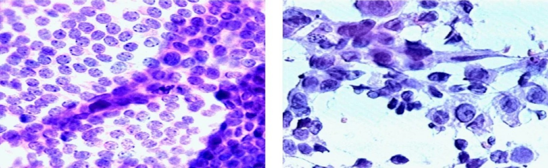
Fine needle aspirate (FNA) of a breast mass is the type of data which this research focuses on. FNA is a type of biopsy performed on breast lesions that collects tissue and fluid samples, from which various attributes of the body cell nuclei, such as compactness, fractal dimension, and area, can be gleaned. Two examples of FNA from the work of Sizilio et al.⁶  are shown in Figure 1. Biopsies are often used to make a final, definitive cancer diagnosis⁷.

Data-Enabled Learning Based Breast Cancer Diagnosis

The introduction of machine learning (ML) and artificial intelligence (AI) processes can reduce difficulties in traditional diagnosis methods. The automated nature of these prediction algorithms greatly increases efficiency, reducing the time and money required of a patient to receive the treatment they need. In addition, ML algorithms have shown the ability to detect tumors in early stages of development that experienced doctors were unable to point out. The development of these algorithms could aid inexperienced medical workers and decrease reliance on experts, making proper breast cancer diagnosis more accessible for all patients⁸.

Related Work for ML in Breast Cancer Diagnosis

Recently, numerous research studies have explored the usage of ML techniques in breast cancer diagnosis, with most works focusing on the type of classification algorithm used for diagnosis. Khalid et al. proposed a deep learning model to diagnose breast cancer using FNA data⁸; they utilized a 3-module process for feature selection: removal of low-variance features, univariate feature selection, and recursive feature elimination. They compared 6 different categorization models: the random forest (RF), decision tree (DT), k-nearest neighbors (KNN), logistic regression (LR), support vector classifier (SVC), and linear support vector classifier (linear SVC). The research heavily focuses on evaluating the FNA data, using detailed metrics to describe the correlation, distribution, etc., of each feature. The study found that among those classifiers not including a DNN, RF was the most effective classifier, attaining an accuracy value of 96.5%; this is a low value compared to the accuracy that can be attained with deep neural networks (DNNs), described later, suggesting that overly complex algorithms and classification methods are not necessarily the superior methods of diagnosis with machine learning. The DT method achieved an accuracy of 93.9%, 92.3% for LR, 92.1% for KNN, 89.5% for linear SVC, and 87.1% for SVC. Using these accuracies, this research study concluded the relative effectiveness of each model as indicated by its relative accuracy value.

In a similar research work by Mustapha et. al, also with the same dataset as Khalid et al., the 5 classification models of support vector machine (SVM), RF, LR, KNN, and NB are compared⁹. The research concluded that SVM was the best model for the early detection of breast cancer with this dataset, followed by KNN, LR, RF, and NB. They found that SVM achieved an accuracy of 99%, KNN 98%, followed by LR, RF, and NB with 97.5%. These accuracies are comparable to the accuracies that can be achieved with a DNN, such as the one utilized in this paper. In addition to the various models used, this work also implemented principal component analysis (PCA) to preprocess the data, and the preference ranking organization method for enrichment evaluations (PROMETHEE) method as a multi-criteria decision-making method (MCDM) to evaluate various criteria in order to determine the best model.

This result clashes with the result found by Khalid et al. in the prior research study presented; with the same dataset used, Khalid et al found that KNN was one of the worst performing models, only achieving an accuracy of 92.1%, while Mustapha et al. found that KNN was one of the best, with an accuracy of 98%. The other results for the same models compared varied similarly among both studies, despite the fact that both used the same dataset. One of the only differences that could account for the much higher accuracy values achieved in the work of Mustapha et. al could be the usage of PCA for preprocessing, which was not implemented in the work of Khalid et. al, underscoring the importance of feature processing research. Another difference could be differences in hyperparameters used, such as learning rate, batch size, and others. However, exact information on these hyperparameters are not given in the work of Khalid et al., making side-by-side comparison in this aspect difficult.

Either way, these contrasting results suggest that the performance of the type of classifier used can depend on many factors and moving parts that can influence each other in many ways, even causing large accuracy differences for the same model on the same dataset, as shown in the previous comparison. Therefore, it would also be valuable to not only focus on these aspects of breast cancer diagnosis with ML, but also other components of the model, such as feature preprocessing. This is the primary motivation for the work of this research on feature processing techniques.

In the vein of evaluating methods of classification, however, many review articles evaluating the wide variety of methods have been published in recent years. Fatima et al. comparatively reviewed many machine learning techniques for breast cancer diagnosis¹⁰, while Yue et al. provided a detailed explanation of the proficiency and usage history of multiple popular techniques¹¹. In particular, both review articles came to the conclusion that the Artificial Neural Network (ANN), which has long been used for diagnosis, is still a reliable method, and often can keep up with other, more novel algorithms, including KNN, NB, and SVC–even exceeding them in performance with the application of other neural network design techniques. The reliability and abundance of supporting references for ANN usage is a primary factor behind the usage of an Multi-Layer Perceptron (MLP), a type of ANN, in this research. The simplicity and relative ease of understanding for the architecture of an ANN allows the main focus of this research to focus on the combination of feature processing techniques to improve accuracy.

Related Work for Feature Extraction Methods in ML Algorithms

Research on feature processing methods for machine learning approaches for diagnosing breast cancer is notably less common; Shafique and Rustam, et al. evaluated multiple feature pre-processing techniques for breast cancer diagnosis using FNA data: principal component analysis (PCA), singular value decomposition (SVD), and chi-square⁷. The researchers also compared a variety of classification approaches: RF, SVM, Gradient Boosting Machine, LR, and KNN. The method for providing a reference accuracy without any feature processing techniques is applied on all models to be tested, and is a guiding outline for the methods used in this research. Then, the accuracy of each model–when each feature processing technique is used to select the 10, 15, and 25 most important features from the FNA data–is evaluated. Their results showed that performance of every model improved when fewer features were used, making the conclusion that even when there were more features, they were not necessarily useful for diagnosis. This result is a significant motivation behind the usage of PCA in this research to evaluate accuracy improvements. However, this research does not evaluate the performance of feature processing techniques when applied to an ANN or DNN, primarily utilizing other models like KNN and RF. In addition, this research does not evaluate the impact of multidimensional scaling (MDS) on the accuracy of any of the models. The implementation of MDS into breast cancer tumor classification could provide improvements in accuracy, especially when combined with linear methods that have already been proven to be successful, like PCA.

MDS has already been used in several ML applications; Li et al. analyzed dimensional reduction for nonadiabatic dynamic systems–critical in photophysics and photochemistry–using classical MDS, showing that classical MDS illustrated the nonadiabatic system dynamics well, resulting in a successful reduction of dimensions for a more robust analysis of the systems¹². In the area of cancer research, Boldrini et al. used MDS to analyze expression levels of gene groups involved in various aspects of prostate cancer progression¹³. MDS was able to reveal clusters of gene relationships that provided better understanding of each group’s role in the cancer progression.

Non-metric MDS (NMDS) is not traditionally used for machine learning algorithms utilizing quantitative data, because, as will be explained in the Methodology section, NMDS preserves the relative ranks, or orders, of dissimilarities within data, while extracting data features in another dimension. It does not focus on preserving the numerical values of dissimilarities like metric MDS, so metric MDS is far more commonly used for quantitative data than non-metric MDS. This research provides an opportunity to address that gap. A few studies have already shown that NMDS has been able to find distinct relationships and groups within data that could not be found by PCA without heavy pre-processing. Taguchi et al. used NMDS to analyze relational patterns, such as cell-cycle phases, among high-dimensional gene expression time series data, concluding that traditional methods like PCA were not able to capture finer relationships like NMDS without data preprocessing; in fact, the results from PCA were distorted and unclear¹⁴.

Feature Processing Research Impact for Breast Cancer Diagnosis

As shown above, most research efforts focused on ML for breast cancer diagnosis thus far have focused on the type of classification algorithm used, such as Support Vector Machine (SVM), Decision Tree (CART), Naive Bayes (NB) and k Nearest Neighbors (kNN), and more, in order to improve accuracy. The increasingly complex nature of these algorithms and large neural networks are difficult to interpret and adapt to new developments, and also require large amounts of training time. Thus, the usefulness of the specific type of ML algorithm used, as shown by simulations, may be overestimated in real-world scenarios. A focus on feature processing, as in this research, would be more beneficial.

In the specific realm of feature processing for ML, research has been done displaying the potential of PCA and NMDS to improve the capabilities of models, and accurately depict relationships within the data for clustering and analysis purposes^7,12,13,14. However, research on this is still very limited for breast cancer diagnosis specifically, and there is also a large research gap in researching the impact of a combination of feature processing techniques to improve ML models, especially for nonlinear and linear methods, which have been shown individually to be effective.

Thus, this research is focused on linear and nonlinear feature dimensionality analysis, termed LINDA, to reduce overfitting and increase prediction accuracy. This paper will analyze how the number of features fitted through the model using these techniques affects the accuracy of diagnosis, and make novel investigations into feature processing to utilize pertinent linear and nonlinear relationships present in data. The effectiveness of these methods will be compared against the standard MLP approach, which has been shown to be an effective algorithm for diagnosis on its own as compared to other methods^10,11, and the effectiveness of each single feature processing method on its own.

The importance of this work is twofold; first, it explores a field outside the differences between specific ML models for classification, instead providing a view of a more productive method of improving the field as a whole: feature processing, which can be incorporated with any model. Second, it explores the potential of combining feature processing methods to accurately describe relationships in breast cancer FNA data. Crucially, the work of Shafique et al. shows how using a linear feature processing method, PCA, to streamline and reduce the number of features allows models to better utilize relationships in data, improving performance⁷. This work expands on theirs by exploring the combination of PCA with nonlinear feature processing, which has also individually shown to be useful in ML applications, to describe relationships in data. In this way, we focus on improving the reliability and versatility of ML methods for diagnosis, as well as accuracy, with feature processing methods that can be adapted and used for many different models that consistently improve the usability of features for accurate diagnosis.

Breast Cancer Background Information

Breast Cancer Symptoms and Diagnosis Process

Breast cancer is a disease depending on characteristics that vary from patient to patient, including but not limited to: age, hormone levels, high BMI, and postmenopausal hormone therapy. These factors, along with the results of potentially multiple screening methods, are utilized by medical experts to perform diagnosis¹⁵. Broadly, breast cancer tumors can be characterized as either malignant or benign. Other factors gleaned from diagnosis such as the stage of breast cancer, the need for continued testing, and the types of additional care that may be required, are equally important conclusions that a medical professional must make during the diagnosis process. This research focuses, however, on identifying the malignancy or benignity of tumors.

Benign tumors are non-life-threatening lumps of cells that are not cancerous; they grow slowly and present a very low risk of metastasizing to other parts of the body. Most breast lumps identified in biopsies are benign. 90% of these benign cases are caused by a subtype of breast cancer called ductal carcinoma in situ (DCIS), while the less rare lobular carcinoma in situ (LCIS) is thought to increase risk of developing malignant breast cancer. Malignant tumors are life-threatening breast lumps that present a high risk of metastasizing to other parts of the body, decreasing the chance of survival for the patient⁷. Thus, the identification of the malignancy or benignity of a tumor is exceedingly important in the potentially life-saving diagnosis process.

Dataset

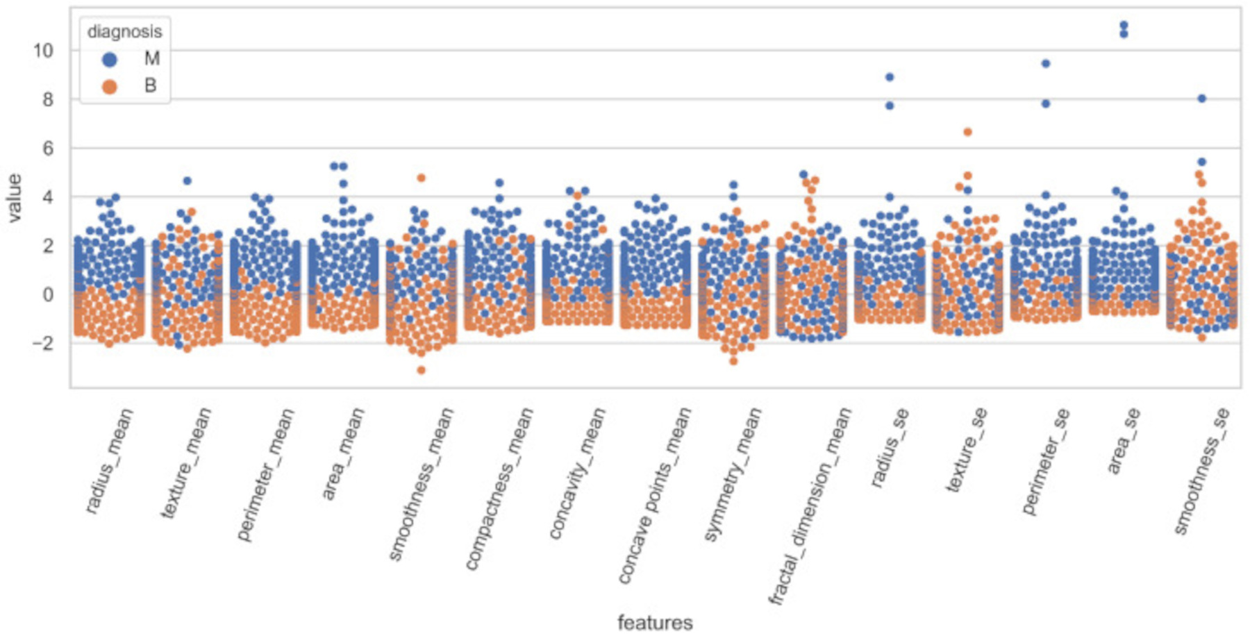
The dataset used in this research is the Wisconsin Breast Cancer Dataset (WBCD) of FNA data, obtained from the UC Irvine Machine Learning Repository¹⁷. The dataset consists of 30 distinct features. Each of the 569 data samples is labeled as benign (B) or malignant (M), with the dataset having 357 benign and 212 malignant tumor samples in total: 62.74% benign, and 37.26% malignant. A representation of the dataset, directly sourced from the work of Shafique et al.⁷, is shown in Figure 2.

For each cell nucleus, ten real-valued features are computed: radius, texture, perimeter, area, smoothness, compactness, concavity, concave points, symmetry, and fractal dimension. For each of the 10 features, the mean, standard error, and worst (the mean of the three largest values) of these features are computed for each cell nucleus, resulting in a total of 30 features.

Methodology

This section will first discuss the linear and nonlinear feature processing techniques, PCA and NMDS, used for LINDA in this research. Next, the main methodology of the experiments will be discussed.

Principal Component Analysis (PCA)

PCA is traditionally used as a dimension reduction technique that allows for better visualization of high-dimension data, but it can be used in ML applications to reduce the number of features to a subset that is representative of the entire dataset, while preserving important relationships within data for prediction. For this research, the PCA module from the scikit-learn decomposition library was used. The fit and transform methods were used from this module.

PCA reduces feature dimensions by finding principal components that each attempt to capture the maximum possible amount of variance in the original data, using the eigendecomposition of the covariance matrix of the data¹⁸. If the original data values are represented by an matrix, where is the number of samples and is the number of features, the entire dataset can be represented by this matrix . If is a vector of length , the variance of a linear combination of the columns of using is given as , where is the sample covariance matrix of the dataset, and represents the transposed version of . To maximize the variance, a vector of length should be obtained that represents the new, reduced features, to maximize . To ensure a meaningful solution, it is required that (the total sum of squared weights).

From the resulting optimization equation, it follows that must equal . Here, represents an eigenvector of the covariance matrix , and the corresponding eigenvalue. The covariance matrix has exactly real eigenvalues, and PCA aims to capture the largest eigenvalue () and corresponding eigenvector , since eigenvalues are the variances of the aforementioned linear combinations. These linear combinations, , represent the principal components of the dataset. As a result of PCA, the principal components are uncorrelated, and each attempts to capture the maximum possible amount of information in the original data.

The PCA model used to extract features from testing and training data was only trained on the training data, to ensure blindness to the validation dataset.

Non-Metric Multidimensional Scaling (NMDS)

Non-metric multidimensional scaling (NMDS), extracts new features nonlinearly¹⁹. The goal of NMDS, like PCA, is often to reduce the dimensions of data to facilitate better comparison and visualization. The linear counterpart of NMDS is metric MDS, which is also used to visualize data in lower dimensions. For this research, the MDS module from the scikit-learn decomposition library was used, with the metric argument set to False. n_init, the number of times the algorithm would be run, was set to 4; the maximum number of iterations was 300; and the pairwise distances were Euclidean.

NMDS begins with a dissimilarity matrix; its goal is to map the original data values into the given lower dimension, in a way that preserves the ranks, or relative orders, of dissimilarities as much as possible²⁰.

For the form of NMDS used in this research specifically, a dissimilarity matrix using the pairwise Euclidean distances between data points is used to fit the NMDS model. To generate the new, lower-dimension features, a set of randomly generated points is created in the lower dimension space. The dissimilarities for the points in this lower dimension space are calculated using Euclidean distances as well.

Then, a monotonic regression is used to transform the dissimilarities into values that describe only the ranked order of distances. Kruskal’s stress function is minimized using the SMACOF algorithm (Scaling by Majorizing a Complicated Function), in order to find positions for the projected data points that minimize the stress, thereby reflecting the ranked order of dissimilarities. The process iterates repeatedly until convergence.

A limitation of NMDS is that the extension of the method to out-of-sample extensions (OSE) is not possible by conventional means²¹. Unlike PCA, there is no explicit function for NMDS to embed OSE data to an existing space, due to the way NMDS functions mathematically–by moving the lower-dimension points around in the lower-dimension configuration space while minimizing a stress function. This is an issue for several reasons. One is that the computational cost to run the NMDS algorithm every time new data is incorporated into the original dataset is too high to be feasible for realistic usage. In addition, it is not possible to separate a dataset into training and testing data, fit the NMDS model to the training data, then transform the testing data with the fitted model; without a proper OSE method, the NMDS model can only be fitted on the entire dataset, allowing it to “peek” at the testing data, rendering the resulting testing accuracy measurements unreliable.

To solve this problem, the artificial neural network (ANN) method from Herath et al. was used²¹. This solution frames the OSE problem as a predictive modeling problem. First, the standard NMDS was applied on the training data only, obtained from the original train-test split, obtaining N points. The testing data was not used to train this ANN, ensuring there was no “peeking.” A set of landmarks L was randomly chosen from these points, to represent the current configuration space. The input data for the ANN were Euclidean pairwise distances between the set of landmarks L and the original points from the untransformed training data, while the output training labels were the set of N points obtained from NMDS.

The ANN, also a MLP, was constructed with 3 fully connected hidden layers with 128, 64, and 32 neurons respectively, with the ReLU activation function, and trained with the mean absolute error loss function and the Adam version of stochastic gradient descent, for 500 epochs, with a learning rate of 0.001, and a learning rate scheduler with a minimum learning rate of 0.0001 and a patience of 10. The train/test split was 80/20, the batch size was 32, and 200 landmarks were used. The resulting model was able to take in the pairwise Euclidean distances between the landmarks and a new OSE data point measured in the higher-dimension space as input, and return the embedding of the new data point in the existing NMDS configuration space. Observing the point errors of embedding out-of-sample data using this method, the NN model is seen to approximate the mapping of a new point with few landmarks producing a small error²¹. It produces consistently good results even with small numbers of landmarks, demonstrating how this method is effective for providing out-of-sample NMDS extensions for existing data.

Combination of PCA and NMDS with Statistical Testing

In this research, the accuracy metric, or the number of correctly predicted labels divided by the total number of labels, will be used to evaluate the performance of models. For classification, regardless of the type of feature used, a DNN, in the form of a 6-layer MLP with a flattening layer, followed by 6 hidden layers with 4 neurons each, was trained for 8000 epochs using binary cross-entropy and the Adam optimizer, with an initial learning rate of 0.001 and a learning rate scheduler with a minimum learning rate of 0.0001. The train/test split was 80/20One dropout layer (0.2) and ReLU activation function were used per hidden layer to mitigate overfitting and vanishing gradients. A sweep over 2–12 layers and 2–12 neurons identified 6 hidden layers × 4 neurons per layer, as optimal, comparing the prediction accuracies with the original 30 features. It provided a high baseline accuracy of 98.1%, averaged across multiple random seeds, as well as 10 baseline accuracy values for a set of 10 different random seeds.

To compare the efficacy of this smaller model with larger, standard architectures with up to 256 neurons per hidden layer, 3-hidden layer tests were also run with 64 neurons per layer; 128 neurons per layer; 256 neurons per layer; 64, 128, then 256 neurons; and 64, 128, then 64 neurons. Otherwise, the same hyperparameters as above were used. The results of this sweep are shown in Table I.

Standard 3-Layer MLP Architecture Tested	Accuracy
64-64-64	97.4%
128-128-128	96.5%
256-256-256	95.6%
64-128-256	97.4%
256-128-64	97.4%
64-128-64	97.4%
128-256-128	96.5%

As shown in Table I, none of the accuracy values for any of the standard architectures with a number of neurons per hidden layer spanning from 64 to 256 are as high as the accuracy attained with a smaller 6-layer MLP with 4 neurons per layer, at 98.1%. This accuracy is comparable with the state-of-the-art values in numerous research studies, making it a good basis for comparison after adding preprocessing. The high accuracy combined with the more compact size of the smaller MLP makes the MLP the best choice for the classification model in this research.

As shown in Figure 3, LINDA combines a varying number of PCA features and a varying number of NMDS features to create the final feature set. The ability of these combined features to describe relationships within the data is evaluated by examining the accuracies of each combination of features, with the number of NMDS and PCA features both ranging from 0-15 over 10 random seeds. From these 256 different combinations, the best-performing 16 combinations were also evaluated using the Wilcoxon signed-rank test²², with the combination of features varying from 2 total features to 30 total features, over 10 random seeds. There were 2 types of statistical tests performed: one for comparison with the 30-feature model, and the other for comparison with the PCA-only model. Each type of test compared 10 combined-feature accuracy values with the set of 10 baseline accuracies obtained from either the 30-feature or PCA-only model; each corresponded to the same set of 10 random seeds. There were 16 different sets of accuracies to test for the baseline model, and 15 different sets for the PCA-only model, as the scenario where the number of NMDS features equaled 0 was not counted. For each individual test, a P-value, representing the likelihood of observing a difference in signed ranks at least as significant as in the sample, was calculated.

The null hypothesis for both tests was that the median of the population of differences between the baseline accuracy and the combined-feature accuracy was 0, and the alternative hypothesis was that it was not 0. The assumptions and conditions were satisfied for both tests: the set of random seeds and the random seed for the train-test-split for both models were the same, so they were treated as paired data; the differences were quantitative and able to be ranked; the pairs were independently trained from one another; and the skew of the distribution of differences was calculated during the test and found to be less than 1 for all but a few pairs for both tests, which were removed from consideration for the tests by automatically setting the P-value to 1. This is because the distribution of differences must be symmetric, so that they can be fairly evaluated; skew is a way to measure this necessary symmetry. The significance level for both tests was 0.03, which is quite low, to minimize the chance of Type I errors.

The performance of each individual feature extraction method, when not combined with the other, were also compared along with the performance of combined feature extraction methods.

Results

In this section, optimal LINDA, or the best combination of NMDS and PCA features will first be discussed, by comparing testing accuracies using the methodology described in the previous section. The performance of the optimal synthesis of NMDS and PCA will be compared to the performance of both individual feature extraction methods, as well as the 30-feature baseline. Finally, the P-values resulting from the methodology will be compared and discussed.

Optimal Combination of NMDS and PCA Features

Using the procedure for LINDA described in the Methods section, the number of PCA features was varied from 0 to 15, and the number of NMDS features was varied from 0 to 15, resulting in 256 possible feature combinations. The 256 testing accuracy values from these feature combinations were averaged across the 10 random seeds, resulting in a final set of 256 accuracy values, which is shown in Figure 4.

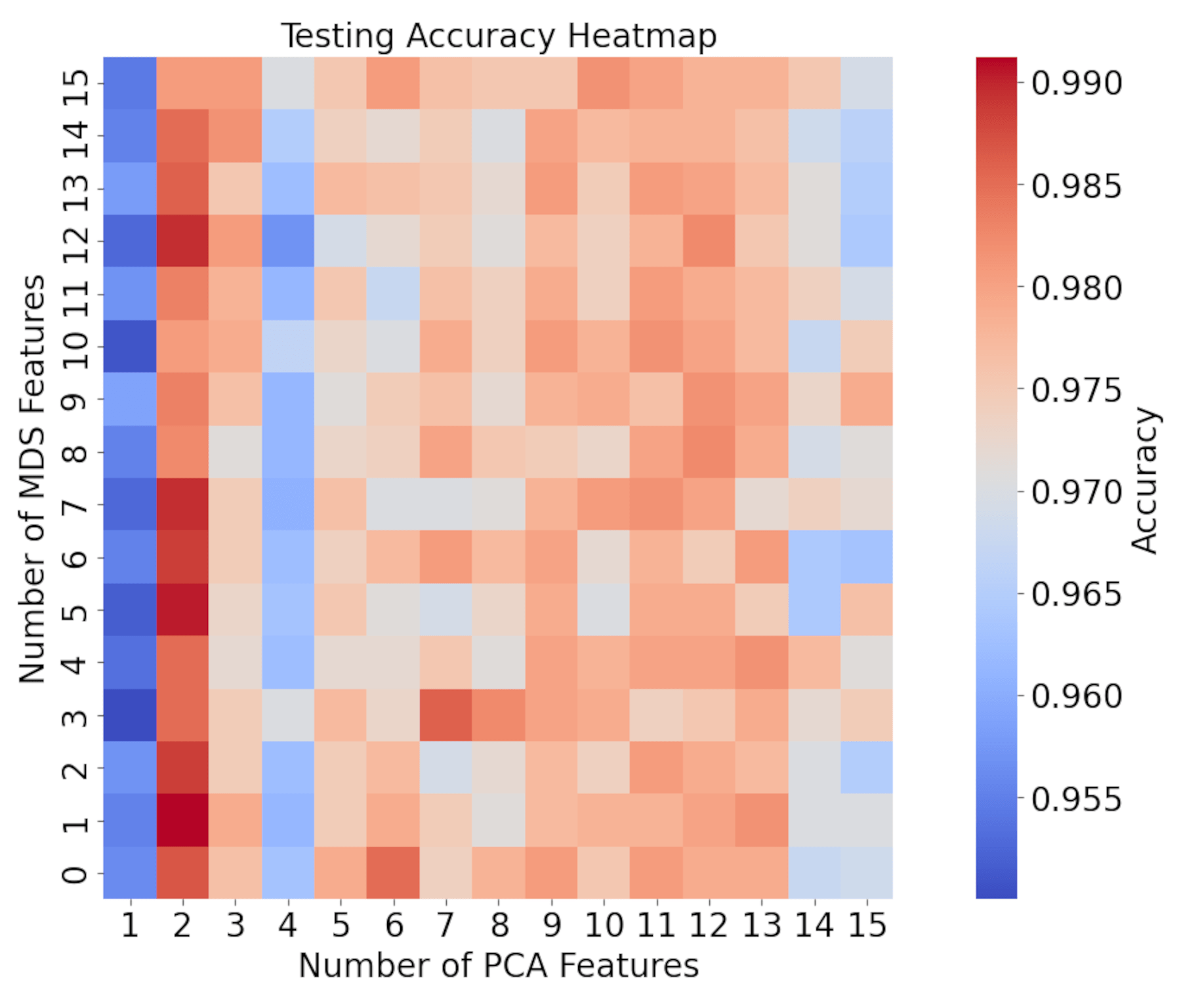
The accuracy values for NMDS only, (when the number of PCA features is 0) are not shown in the plot, due to their consistently low values of 63 to 65% that cause interpretation of the rest of the heatmap to become very difficult if included. These values will be explained later on. As seen in Figure 4, a combination of 2 PCA features with any number of NMDS features resulted in the highest testing accuracies, with some over 99%, exceeding the baseline accuracy of 98.1% by around 1%. The accuracy values stayed relatively constant as the number of NMDS features changed, and increased around the range of 9-12 PCA features.

Since the highest testing accuracy values were present when the number of PCA features was 2, the number of 2 PCA features was chosen to be combined with an increasing number of NMDS features, in order to evaluate the true degree to which the combination of PCA and NMDS improved the reference testing accuracy, from 1 to 28, to perform further testing. 

Impact of Combined and Individual Feature Extraction Techniques

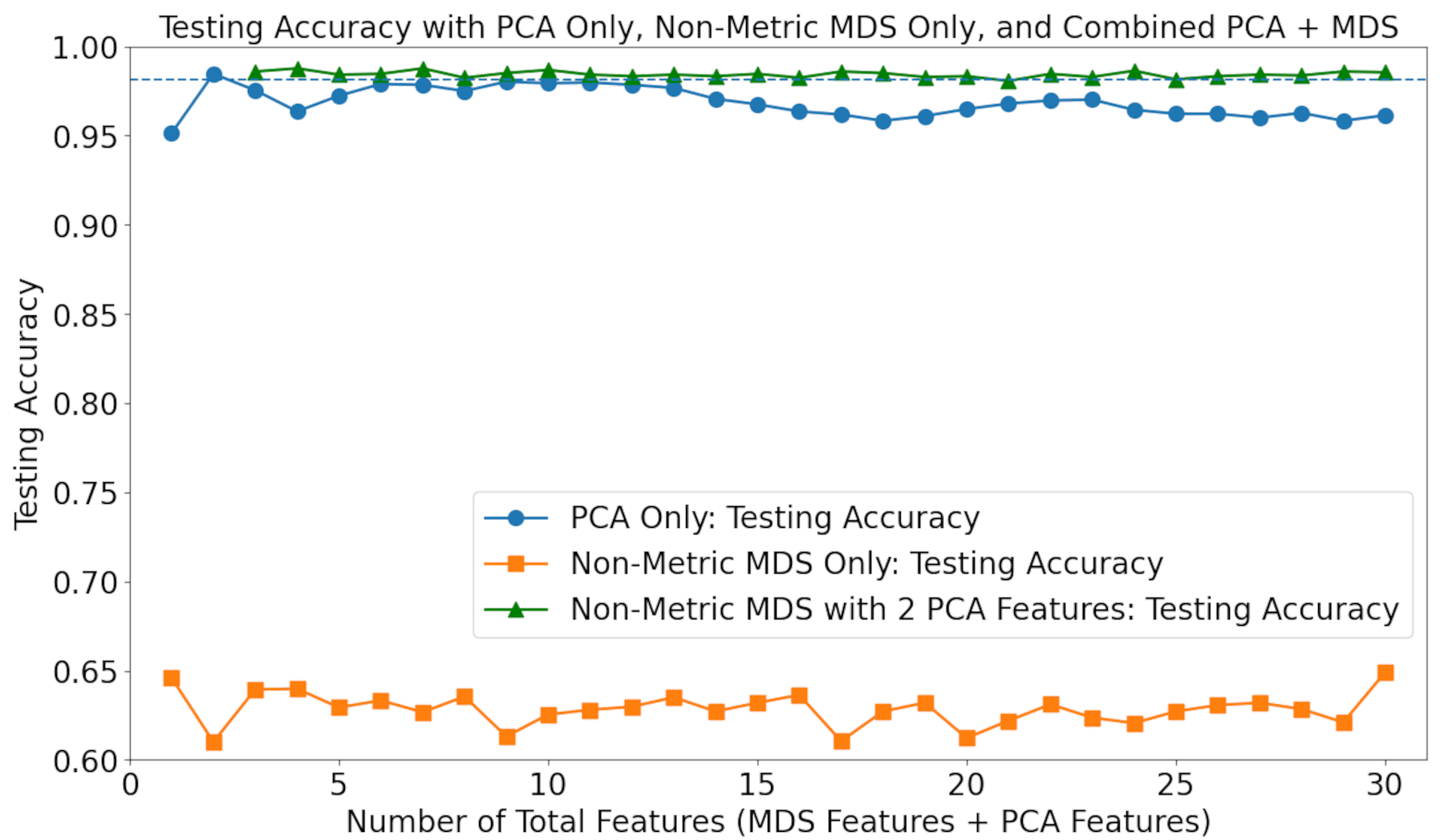
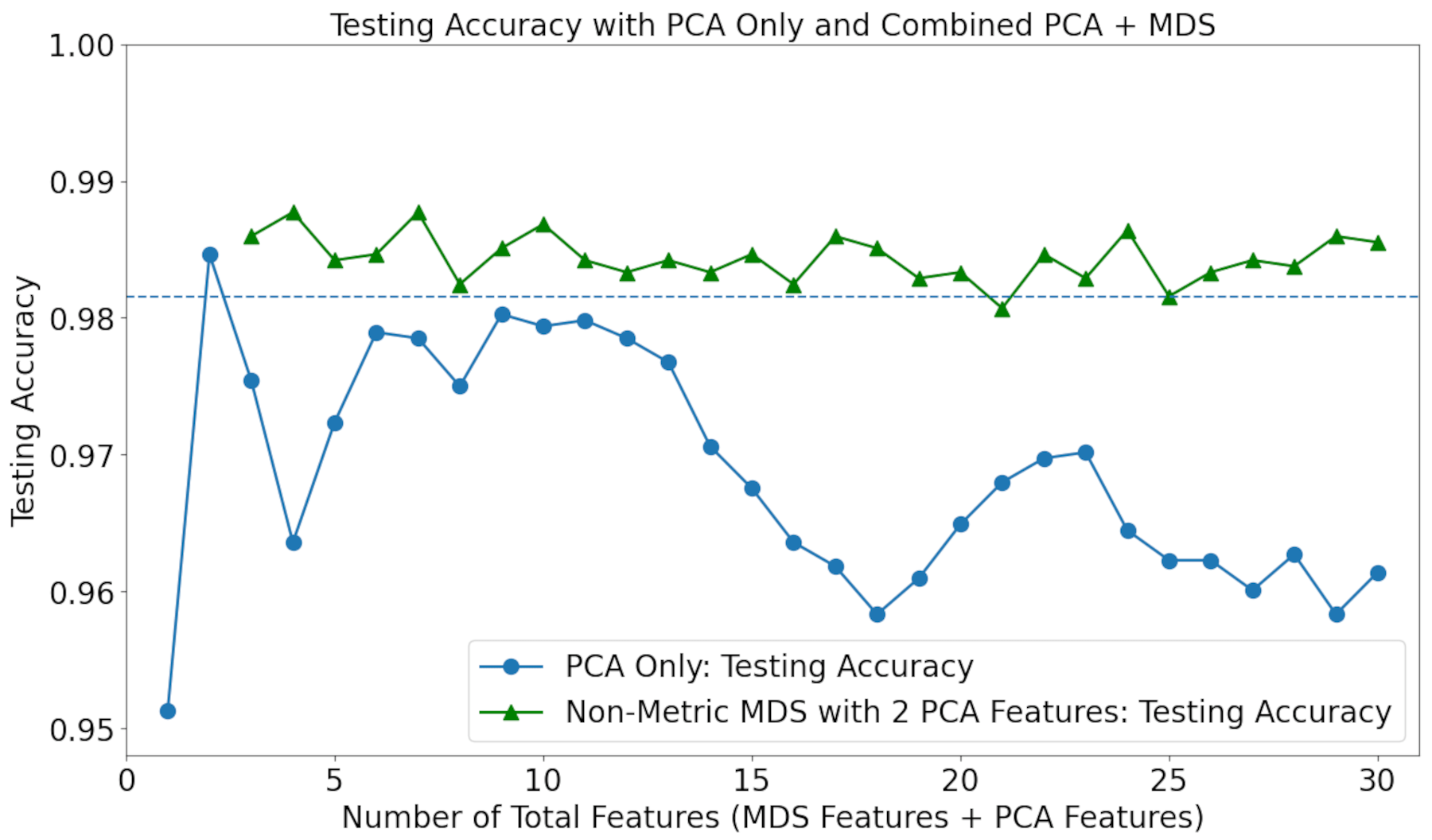
Since NMDS with 2 PCA features was shown to result in high accuracy, the number of 2 PCA features was chosen to be combined with an increasing number of non-metric features. The individual capabilities of PCA and NMDS were also evaluated. The results are shown in Figure 5.

It can be seen that the accuracy values for non-metric MDS only are consistently low. The usage of PCA only resulted in worse accuracy for virtually all numbers of features, compared to when no feature processing methods are used, yet still far higher than those for MDS only; the true improvement in performance results from the combination of PCA with NMDS. Combining the two feature processing techniques with LINDA, the best performance of all was achieved, with up to a 0.5% increase in accuracy compared to the 30-feature baseline, and up to a 3% increase in accuracy compared to the PCA-only baseline.

Statistical Significance Testing

Since it has been established that feature combinations with 2 PCA features and a varying number of NMDS features are optimal, resulting in the most significant accuracy improvements in the baseline model, the 16 combinations tested in the first type of statistical test described in the Methodology section comprise those combinations. The 16 resulting P-values are shown in Table II. When the Bonferroni correction is accounted for, the threshold for significance for the P-value becomes 0.03 divided by the number of tests, 16: 0.0019. The following observations can be made:

• None of the feature combinations here, compared to the baseline model, are shown by this statistical test to provide a significant accuracy improvement, as none of the P-values are below 0.0019.
• However, some are close, such as the P-value for 1 NMDS feature combined with 2 PCA features. 

Number of NMDS Features	P-Value	Number of NMDS Features	P-Value
0	0.1178	8	0.6261
1	0.0041	9	0.5561
2	0.0433	10	0.6405
3	0.3885	11	0.5429
4	0.3613	12	0.0167
5	0.0069	13	0.2464
6	0.0266	14	0.0786
7	0.0167	15	0.6655

The P-values resulting from the second type of test described in the Methods section are shown in Table III. Again, with the Bonferroni correction, the threshold for significance for the P-value becomes 0.03 divided by the number of tests, 15: 0.002. The following observations can be made:

• There were far more statistically significant improvements by the feature-combination model over the PCA-only baseline, compared to the baseline model trained on all 30 features, as seen by the much higher number of significant P-values.
• The P-values for 2 PCA features with 2, 7, 12, and 14 NMDS features are less than 0.002; these feature combinations showed a statistically significant improvement over the PCA model. 
• These observations align with those from previous sections.

Number of NMDS Features	P-Value	Number of NMDS Features	P-Value
1	0.0035	8	0.3994
2	0.00098	9	0.2615
3	0.0086	10	0.3829
4	0.2615	11	0.1024
5	1.0	12	0.00098
6	0.0037	13	0.0029
7	0.0019	14	0.00098
		15	0.0083

Performance Metrics using LINDA

Considering the results of the previous sections, we again evaluate the performance of feature combinations with 2 PCA features, which are shown to be the best combinations for LINDA. To provide perspectives other than accuracy, any commonly used metrics are utilized, shown in Table IV, to demonstrate the excellent performance of the model with LINDA²³. In addition, the ROC-AUC is also used to provide a score of the model’s ability to distinguish between malignant and benign tumors²⁴.

Metric	Formula	Description
Sensitivity/Recall	TP/(TP+FN)	Scores how well the model diagnoses malignant tumors.
Specificity	TN/(TN+FP)	Scores how well the model diagnoses benign tumors.
Precision	TP/(TP+FP)	Scores the model’s reliability to correctly diagnose malignant tumors.
F1-Score		Scores the model’s ability to balance sensitivity/recall with precision.
False Positive Rate	FP/(FP+TN)	The proportion of benign tumors incorrectly identified as malignant.
False Negative Rate	FN/(FN+TP)	The proportion of malignant tumors incorrectly identified as benign.

The means and standard deviations for each statistic, calculated for each of the 16 combinations being focused on here, are shown in Table V.

Metric	Mean ± Standard Deviation
Sensitivity/Recall	0.9535 ± 0.0240
Specificity	1.0 ± 0.0
Precision	1.0 ± 0.0
F1-Score	0.9760 ± 0.0126
False Positive Rate	0.0 ± 0.0
False Negative Rate	0.0465 ± 0.0240
ROC-AUC	0.9877 ± 0.0115

As seen in Table V, the results of each metric for the 2-PCA feature model are excellent; the sensitivity/recall, F1-Score, false negative rate, and ROC-AUC are very nearly perfect, with means close to 1 or 0 and very small standard deviations, and the model attained a perfect score for specificity, precision, and false positive rate. The model predicted no false positives, missing a single malignant case.

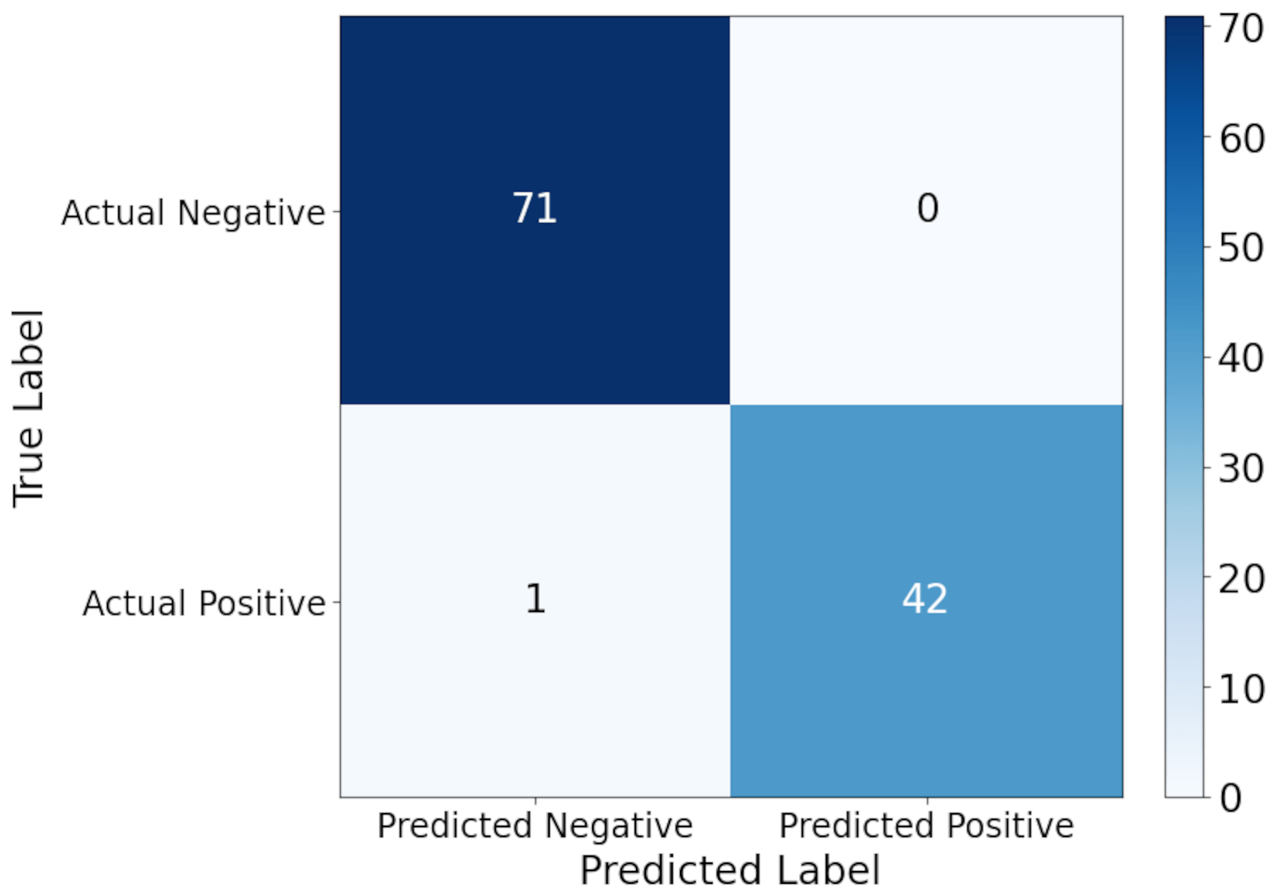
In Figure 6 below, a confusion matrix for the actual and predicted negatives and positives is shown for the specific model with a feature combination of 1 NMDS feature and 2 PCA features. This combination is shown because it consistently showed one of the highest accuracies in Figures 4 and 5, but also produced P-values very close to the significance values in the statistical testing. In addition, with only 3 total features for prediction, it is an example of the power of LINDA to provide excellent results with only 10% of the original number of features. Despite only having 3 input features to use for classification, the model correctly diagnosed all benign cancers, and correctly diagnosed all but one malignant cancers.

Discussion

Despite the individual performances of models with PCA and NMDS feature processing alone being subpar, the combination of NMDS and PCA, with a small number of features derived from PCA combined with features derived from NMDS acting as input to the DNN, resulted in the best performance of all, likely resulting from the complete nature of the relationships that were both best represented with LINDA, allowing for the best diagnosis.

As seen in Figures 4 and 5, the feature combination of 2 PCA features with any number of NMDS features results in consistently high accuracy. Furthermore, the Wilcoxon signed-rank tests, displayed in Tables II and III, prove the actual significance of these higher accuracy values, with P-values less than the significance level with the Bonferroni correction for several feature combinations within the category. Even though there were no statistically significant combinations found for a combination of features compared with the baseline model with 30 features, it can nevertheless be seen in Figure 5 that an improvement over the baseline by the feature combination exists. In the future, more data across a higher number of random seeds, or usage of a different statistical test more suited to this situation could prove useful for resolving this discrepancy.

In Figure 5, it can be seen that the accuracy values for only NMDS were consistently low, regardless of the number of NMDS features. The most likely reason for these consistently low values was that the features, by themselves, did not provide the MLP model any information on relationships within the data that could be used for diagnosis, causing the model to merely learn the configuration of the output labels instead.

The nonlinear nature of NMDS and the usage of the ANN for NMDS out-of-sample extension (OSE) were likely the root cause of these issues. Regardless of the different dimensionalities that the NMDS features were projected into, the ANN used for NMDS OSE likely generalized similarly across them, causing the outputs to be similar as well. In addition, NMDS preserves ranked dissimilarities, not the numerical values of dissimilarities. This type of nonlinear preservation likely did not capture the type of relationships needed by the MLP to classify testing data using NMDS on its own.

For PCA only, compared to when no feature processing methods are used, an accuracy level much closer to, but never on par with the baseline accuracy was achieved, as the PCA-extracted features could not fully encapsulate the relationships needed for classification within the data. In fact, the testing accuracy of the model decreased as the number of PCA features increased. This was likely because the majority of the pertinent relationships in data were preserved in the initial few features, and the addition of new features may have been unnecessary and even detrimental to the model, resulting in higher accuracy for lower numbers of features.

The consistently high performance of the model integrated with LINDA demonstrates that together, NMDS and PCA are able to capture both linear and nonlinear relationships within the data that can improve the model’s accuracy, even compared to using the original features. On their own, PCA and NMDS are unable to capture all these relationships. PCA focuses on preserving the global structure within the data, likely throwing out the finer discriminative features. The first two principal components can capture most of the variance within the dataset, while adding more features only adds noise for the model. NMDS preserves non-linear relationships in local structures through its preservation of the ranked pairwise similarities between data points, but is unable to preserve variance or global structure well.

Combined, PCA and NMDS can be understood to cover the global and local relationships within the dataset, respectively. They complement one another and can holistically represent the data in a space of much lower dimension, and when used in tandem to train the model, allow the model to learn these relationships for classification of testing data.

Additionally, when the LINDA-integrated model is compared with the PCA-only model, there are far more statistically significant improvements other than with only 2 PCA features, as seen in Table III, further demonstrating that the presence of NMDS along with PCA is an improvement over only PCA.

Finally, outside of just accuracy, the abilities of LINDA integrated with the MLP are shown with the excellent evaluation metric values shown in Table V and Figure 6. With a varying number of MDS features combined with 2 PCA features, the mean and standard deviations for each metric were excellent, demonstrating that LINDA has potential to be utilized in a real clinical setting. The false negative rate was a bit higher than the false positive rate, with the 2-PCA, 1-NMDS feature model incorrectly identifying one malignant case as benign. A higher false negative rate is more harmful in a clinical setting, as letting breast cancer go undiagnosed, and therefore treatment unadministered, can pose significant risk. Therefore, optimization to the model to maximize sensitivity at the cost of specificity may be worth ensuring malignant cases are not falsely diagnosed.

A limitation of this research that can be addressed in future work is the need for an extra ANN to allow for OSE for the NMDS model, which increases the complexity of the pipeline and creates further need for computation resources. Additionally, the dataset used is small; the viability of the feature processing techniques should be confirmed using other more expansive datasets. In the future, more exploration of the effects of feature processing techniques on other types of ML models other than DNNs would be beneficial as well.

Conclusion

In this research, a deep neural network (DNN) in the form of a Multi-Layer Perceptron (MLP) was used to evaluate the impacts of combining linear PCA and nonlinear NMDS feature processing, or LINDA, on the accuracy of the model for classifying breast cancer tumors as malignant or benign. The effects of both methods individually and combined were evaluated, with a varying number of features extracted using each, and the resulting accuracies compared. A noteworthy result was that the combined-feature model with as little as 3 total input features was consistently able to produce an accuracy up to 0.5% higher than that of the baseline 30-input-feature model, and up to 3% higher than that of the baseline PCA-only model, and also also achieved near-perfect scores in other performance metrics. . The effectiveness of combining small numbers of nonlinearly and linearly extracted features with LINDA to train a highly accurate diagnosis model demonstrates how small amounts of highly optimized data can achieve comparable accuracy compared to a model with 30 full features. The technique described in this paper of combining nonlinear and linear feature processing techniques can be extended to research in diagnosing other types of cancers and diseases as well. In addition, there is much potential in other feature processing techniques to explore, to continue streamlining the diagnosis process to save as many lives from breast cancer as possible.

References

1. M. Arnold, E. Morgan, H. Rumgay, A. Mafra, D. Singh, M. Laversanne, J. Vignat, J. R. Gralow, F. Cardoso, S. Siesling, I. Soerjomataram. Current and future burden of breast cancer: Global statistics for 2020 and 2040. The Breast: Official Journal of the European Society of Mastology 66, 15–23 (2022). [↩] [↩]
2. S. Mayor. Survival of women treated for early breast cancer detected by screening is same as in general population, audit shows. BMJ: British Medical Journal 336, 1398–1399 (2008). [↩]
3. L. Wang. Early Diagnosis of Breast Cancer. Sensors 17, 1572 (2017). [↩] [↩] [↩] [↩] [↩]
4. E. S. McDonald, A. S. Clark, J. Tchou, P. Zhang, G. M. Freedman. Clinical Diagnosis and Management of Breast Cancer. Journal of Nuclear Medicine 57, 9S–16S (2016). [↩]
5. G. R. M. A. Sizilio, C. R. M. Leite, A. M. G. Guerreiro, A. D. D. Neto. Fuzzy method for pre-diagnosis of breast cancer from the Fine Needle Aspirate Analysis. BioMedical Engineering OnLine 11, 83 (2012). [↩]
6. G. R. M. A. Sizilio, C. R. M. Leite, A. M. G. Guerreiro, A. D. D. Neto. Fuzzy method for pre-diagnosis of breast cancer from the Fine Needle Aspirate Analysis. BioMedical Engineering OnLine 11, 83 (2012). [↩]
7. R. Shafique, F. Rustam, G. S. Choi, I. de la Torre Díez, A. Mahmood, V. Lipari, C. L. Rodríguez Velasco, I. Ashraf. Breast Cancer Prediction Using Fine Needle Aspiration Features and Upsampling with Supervised Machine Learning. Cancers 15, 681 (2023). [↩] [↩] [↩] [↩] [↩] [↩]
8. A. Khalid, A. Mehmood, A. Alabrah, B. F. Alkhamees, F. Amin, H. AlSalman, G. S. Choi. Breast Cancer Detection and Prevention Using Machine Learning. Diagnostics 13, 3113 (2023). [↩] [↩]
9. M. T. Mustapha, D. U. Ozsahin, I. Ozsahin, B. Uzun. Breast Cancer Screening Based on Supervised Learning and Multi-Criteria Decision-Making. Diagnostics 12, 1326 (2022). [↩]
10. N. Fatima, L. Liu, S. Hong, H. Ahmed. Prediction of Breast Cancer, Comparative Review of Machine Learning Techniques, and Their Analysis. IEEE Access 8, 150360–150376 (2020). [↩] [↩]
11. W. Yue, Z. Wang, H. Chen, A. Payne, X. Liu. Machine Learning with Applications in Breast Cancer Diagnosis and Prognosis. Designs 2, 13 (2018). [↩] [↩]
12. X. Li, Y. Xie, D. Hu, Z. Lan. Analysis of the Geometrical Evolution in On-the-Fly Surface-Hopping Nonadiabatic Dynamics with Machine Learning Dimensionality Reduction Approaches: Classical Multidimensional Scaling and Isometric Feature Mapping. Journal of Chemical Theory and Computation 13, 4611–4623 (2017). [↩] [↩]
13. L. Boldrini, P. Faviana, L. Galli, F. Paolieri, P. A. Erba, M. Bardi. Multi-Dimensional Scaling Analysis of Key Regulatory Genes in Prostate Cancer Using the TCGA Database. Genes 12, 1350 (2021). [↩] [↩]
14. Y. Taguchi, Y. Oono. Relational patterns of gene expression via nonmetric multidimensional scaling analysis. Bioinformatics 21, 730–740 (2004). [↩] [↩]
15. E. J. Watkins. Overview of breast cancer. JAAPA 32, 13-17 (2019). [↩]
16. R. Shafique, F. Rustam, G. S. Choi, I. de la Torre Díez, A. Mahmood, V. Lipari, C. L. Rodríguez Velasco, I. Ashraf. Breast Cancer Prediction Using Fine Needle Aspiration Features and Upsampling with Supervised Machine Learning. Cancers 15, 681 (2023). [↩]
17. W. Street, W. Wolberg, O. Mangasarian. Breast Cancer Wisconsin (diagnostic). UCI Machine Learning Repository (1993). [↩]
18. I. T. Jolliffe, J. Cadima. Principal component analysis: A review and recent developments. Philosophical Transactions of the Royal Society A: Mathematical, Physical and Engineering Sciences 374 (2016). [↩]
19. S. De Backer, A. Naud, P. Scheunders. Non-linear dimensionality reduction techniques for unsupervised feature extraction. Pattern Recognition Letters 19, 711–720 (1998). [↩]
20. M. C. Hout, M. H. Papesh, S. D. Goldinger. Multidimensional scaling. Wiley Interdisciplinary Reviews: Cognitive Science 4, 93–103 (2012). [↩]
21. S. Herath, M. Roughan, G. Glonek. High Performance Out-of-sample Embedding Techniques for Multidimensional Scaling. arXiv.org (2021). [↩] [↩] [↩]
22. F. Wilcoxon. Individual Comparisons by Ranking Methods. Biometrics Bulletin 1, 80–83 (1945). [↩]
23. O. Rainio, J. Teuho, R. Klén. Evaluation metrics and statistical tests for machine learning. Scientific Reports 14, 6086 (2024). [↩]
24. Çorbacıoğlu, Ş. K., G. Aksel. Receiver operating characteristic curve analysis in diagnostic accuracy studies: A guide to interpreting the area under the curve value. Turkish Journal of Emergency Medicine 23, 195–198 (2023). [↩]