Investigating the Effect of Active Galactic Nuclei on Their Host Galaxies

November 28, 2025

Abstract

Active galactic nuclei (AGN) are a doorway for astronomers to understand the deep cosmos. This paper gathers evidence to better understand the correlation between AGN characteristics and their surrounding host galaxies. To investigate these correlations, three scientific papers from the past decade and 35 quasar-type Superspectra were analyzed in the form of fits files. The spectra were imported from the Sloan Data Sky Survey and four crucial emission lines were fitted for each of the 35 spectra using Gaussian functions to determine their amounts of hydrogen alpha and beta, nitrogen II, and doubly ionized oxygen (OIII). This investigation revealed that more massive AGN tend to correlate to an overall higher galactic mass, and that Intermediate Mass Black Holes are normally formed in the accretion disk of a Super Massive Black Hole (SMBH). As well, SMBH are not naturally occurring by the process of star life. Finally, increasingly larger AGN result in an increase in central kiloparsec intensity and a decrease in galactic activity radius. This paper provides insight into the intricacies of galactic activity, detailing the complex relationship AGN have with their host galaxies.

Introduction

In modern astronomy, an overwhelming amount of evidence suggests the presence of Super Massive Black Holes (SMBH) in the center of galaxies. High luminosity, compactness, time variability, and spectral energy distribution of AGN are best explained as effects of disk accretion into an SMBH. However, concrete evidence is needed to confirm that gas indeed accretes into a SMBH while inside the event horizon. It is, rather, commonly observed that gas outflows from AGN, causing massive relativistic jets traveling at extremely fast speeds in relation to the speed of light itself. This phenomenon coupled with the sheer amount of electromagnetic radiation it expels allows for astronomers to categorize the SMBH at the center of the galaxy and its corresponding accretion disk, narrow line region (NLR), broad line region (BLR), and relativistic jet as the active galactic nuclei: a nucleus usually only around 1 parsec in diameter which is more luminous than all of the surrounding kiloparsecs combined that form a host galaxy. In recent years, astronomers have posited a correlation between properties of black holes such as angular momentum and mass with the overall size, structure, and level of star formation in the host galaxy. The objective of this paper is to examine published documents and spectra to analyze and better understand the correlation between the characteristics of AGN and the evolution of their respective galaxies.

To answer this central question, this paper will consist of two major sections: a literature review and a data analysis. The literature review section covers the sources’ discussions on the modern understanding of AGN spectra, classification of AGN, and correlations between AGN and their host galaxies. This review also provides academic context to clarify the current understanding of the topic and a further discussion on the correlations that were drawn. The second section will be centered on data analysis with a step-by-step methodology, describing the process by which the results were synthesized.

Academic Context

Aside from dark matter, components of the known universe are present in AGN such as stars, gas, and dust which contribute to their spectra. This literature review and data analysis will focus on optical and broadband spectra as they are relevant tools that characterize AGN and can potentially explain a relationship between the properties of AGN and the evolution of their host galaxies. Below is a brief summary of the subject material that will be analyzed further in this work. This academic context was derived from reading the textbook, An Introduction to Active Galaxies (The Open University, 2016)¹.

Optical Spectra

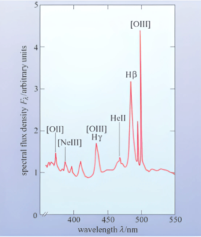
Optical in this context refers to visible light. Optical spectra for galaxies typically consist of flux from stars and emissions from ionized gas clouds. Wavelengths of the optical spectra measure roughly between 380 and 700 nm. Elliptical galaxies have smaller hydrogen II (HII) regions and have an optical spectrum which resembles a star’s spectrum but with fainter absorption lines. A spiral galaxy has both stars and star-forming regions, and its optical spectrum is the composite of its stars and its HII regions which show weaker emissions. Dust, being too cool to appear in optical spectra, often attenuates and dims galactic spectra. Optical light absorption lines also reveal chemical information about the host galaxy. In Figure 1, (below) the optical spectra only covers wavelengths specific to the visible portion of the electromagnetic spectrum. From this spectra, there are unique chemical signatures that can be recognized as each element or compound has a different fingerprint at a specific wavelength. This will be heavily utilized in the later data analysis.

Broadband Spectra

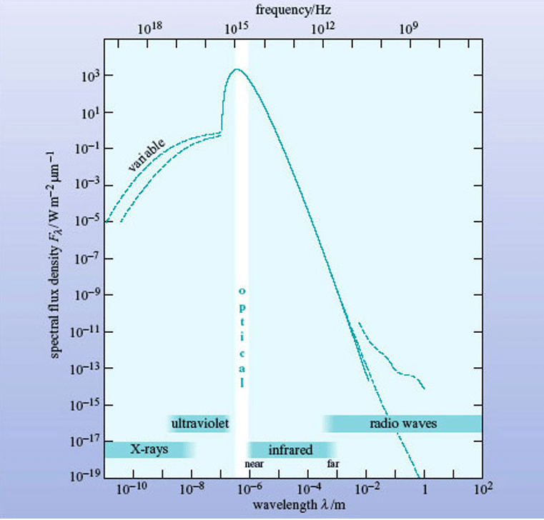
Broadband spectra fully encompass the electromagnetic spectrum and are often plotted using a logarithmic equation. The logarithms are often derived from wavelength measurements. Incorporating all forms of the electromagnetic spectrum into the characterization of a galaxy provides more information about the galactic nuclei’s effect on the host galaxy as well. Broadband spectroscopy will be essential in the data analysis portion when using a BPT diagram. Broadband spectra typically compare the ratios of emission fluxes.

AGN Classification

Classification of AGN by mass and electromagnetic emissions allows connections between AGN and their host galaxies to be better understood. The largest subclasses of active galaxies are Seyfert and quasar galaxies which differ mainly in the radiation they emit. In a typical Seyfert galaxy, the nuclear source emits at visible wavelengths an amount of radiation comparable to that of the whole galaxy’s constituent stars. In a quasar, however, the nuclear source is brighter than the constituent stars by at least a factor of 100. Seyfert galaxies are typically closer to Earth than quasars which in addition to their lower overall luminosity makes them harder to discover from more than several million parsecs away.

Seyfert Galaxies

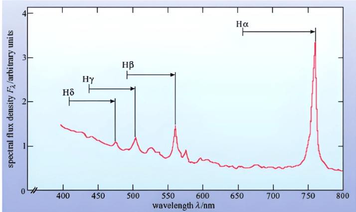
Seyfert galaxies (Seyfert Type 1, Type 2, and LINERS) show an excess of radiation in the far infrared spectrum. Even more remarkably, at some wavelengths, including optical, this excess radiation is variable. Seyfert galaxies are also subclassified into two major types based on the spectra of their broad emission lines. Type 1 Seyferts have two sets of emission line regions, narrow and broad, whereas Type 2 Seyferts have only a noticeable narrow region. This indicates that Type 1 Seyferts have more mass and likely a corresponding higher angular velocity. Figure 3 compares the two types of Seyfert galaxies. There is a noticeable difference between the two where the spectra of the first graph, a Seyfert Type 1 galaxy, is heavier in shorter wavelengths at a higher spectral density. This seems to be consistent with previous ideas that Type 1 Seyferts are more massive and are rotating relatively faster than Type 2s.

Figure 3 | Seyfert Type 1 contrasted with Seyfert Type 2 (optical spectra) – Introduction to Active Galaxies (Open University)¹

Quasar galaxies (Quasars, Blazars, Radio Galaxies)

Thought to be stars when first discovered, quasars are the most luminous type of AGN. Quasars resemble distant Seyfert galaxies with variable luminous nuclei. About 10% of quasars are strong radio sources thought to be powered by jets of material moving at speeds close to the speed of light. Radio and blazar galaxies are two AGN archetypes similar to quasars. Radio galaxies are distinguished by having giant radio lobes fed by one or two emission jets. All three have compact nuclei like Seyfert Galaxies, but their nuclei are variable with broad or narrow emission lines. Blazars exhibit a continuous spectrum across a wide range of wavelengths and emission lines which, when present, are broad and weak.

Figure 4 | Quasar galaxy optical spectra – Introduction to Active Galaxies (Open University)¹

Methodology

Review Paper

Search Strategy & Inclusion Criteria

In order to answer the central question on the existence of a correlation between AGN and the respective structure of their parent galaxy, the following three works were analyzed. Three works were chosen for a pragmatic overview of the central question. The details of each work that regard the central question are documented in this review paper. Additionally, the following works were chosen because of their recency in astronomy and their high citation count.

Relations Between Central Black Hole Mass and Total Galaxy Stellar Mass in the Local Universe Reines et al.² studied 262 broad-line AGN in the nearby universe, using SDSS spectroscopy and searching for Seyfert-like narrow-line ratios and broad H $\alpha$ emission, only using galaxies with a redshift z $<$ 0.055. The authors identify a correlation between SMBH and the size and total mass of the host galaxy. Investigation of this correlation assists in understanding the overall effect of AGN.

Intermediate Mass Black Holes in AGN Disks II. Model Predictions and Observational Constraints McKernan et al.³ delves into the accretion and formation of Intermediate Black Holes (IMBH) inside the disk of a galactic nucleus. This paper lends insight on the formation of black holes of intermediate size and on the chemical compounds that formed them. It also provides an understanding of whether IMBHs contributed to galactic evolution.

Fueling Active Galactic Nuclei I. How the Global Characteristics of the Central Kiloparsec of Seyferts Differ from Quiescent Galaxies Hicks et al.⁴ examines the inner parsecs (pc) of central SMBH, then raises a hypothesis about Seyfert galaxies being cold relative to other galaxies. This paper initially investigates the similarities and differences between inactive or quiescent galaxies and the most common type of AGN, a Seyfert galaxy. The paper then contrasts the two galaxy types within distances of 1, 50, 100, 200, and 500 parsecs.
These three papers function as a good reference for investigating the correlation between AGN characteristics and galaxy evolution.

Information Extraction & Synthesis

To elaborate further on the contents of the analysis, the details of each work that regard the central question are documented in this review paper. This includes figures, equations, and discussions that offer evidence of a correlation between Active Galactic Nuclei and their host galaxies. Takeaways will be discussed at the end of the paper analysis, compared with one another and correlations will be drawn if there are similarities between multiple works.

Paper Analysis

Relations Between Central Black Hole Mass and Total Galaxy Stellar Mass in the Local Universe Reines et al.²

Reines et al.² collected a sample of AGN emissions and then calculated the mass of black holes for comparison. A focus on other objects such as dwarf galaxies containing AGN, reverberation-mapping of AGN, and galaxies with dynamically detected black holes form the remainder of this study. Reines et al.² constructed a sample of broad-line AGN by analyzing Sloan Digital Sky Survey (SDSS) spectra of approximately 67,000 emission-line galaxies, searching for objects exhibiting broad hydrogen alpha emissions and simultaneously comparing them to their hydrogen beta emissions. SDSS focuses on galaxies in the local universe: redshift z $\sim$ 0. Figure 5 below is a spectral analysis of the galaxies in the Sloan survey sampled in this paper.

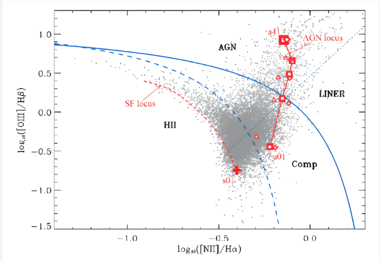
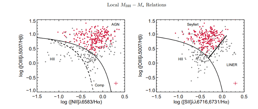Figure 5 | Reines et al.² – Narrow-line diagnostic diagrams for sources with detectable broad H $\alpha$ emission. These are produced using the classification scheme outlined in Kewley et al. (2006). The sample of broad-line AGN is restricted to objects with narrow line ratios placing them in both the AGN region of the [OIII]/H $\beta$ vs. [NII]/H $\alpha$ diagram and the Seyfert region of the [OIII]/H $\beta$ vs. [SII]/H $\alpha$ diagram (red points). The typical error for the red points is shown in the lower right corner of each plot.

With AGN emissions data, Reines et al.² shifted focus to black hole luminosity. The mass of the black hole is to be proportional to $\frac{[R\times(V2-V1)^2]}{G}$ . It also states that the average gas velocity is inferred from the width of a broad emission line, usually looking at its levels of hydrogen $\beta$ . Reines et al.² estimated black hole masses from their sample of broad-line AGN using the single-epoch virial mass estimator given by equation 5 in Reines et al.². Equation 1 below was derived following the approach outlined in Greene & Ho (2005) for using the broad H $\alpha$ line but incorporates the updated radius-luminosity relationship from Bentz et al. (2013).

(1) $\begin{equation*}\log \left( \frac{M_{\rm BH}}{M_\odot} \right) = \log \epsilon + 6.57 + 0.47 \log \left( \frac{L_{\rm H\alpha}}{10^{42}\ \rm erg\ s^{-1}} \right) + 2.06 \log \left( \frac{\rm FWHM_{H\alpha}}{10^{3}\ \rm km\ s^{-1}} \right)\end{equation*}$

Reines et al.² utilized an equation to calculate the total stellar mass of the host galaxy without the AGN contribution, using this equation to compare the mass of the black hole and the host galaxy to uncover the desired correlation. The equation below removes the mass calculation of the AGN contribution. Host-only magnitudes (corrected for galactic reddening)

are used to estimate galaxy stellar masses with a color dependent mass-to-light ratio. Below is the dependent mass-to-light ratio from Zibetti et al. (2009).

(2) $\begin{equation*}\log \left( \frac{M}{L_i} \right) = 1.032\, (g-i) - 0.963\end{equation*}$

Finally, Reines et al.² graphed the full width at half maximum (FWHM) of the galaxies’ broad hydrogen alpha (left panel), graphed their luminosity, and then calculated the distribution of said galaxies using the radius-luminosity relationship.

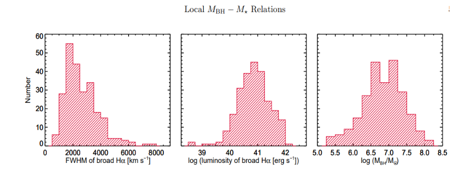Figure 6 | Reines et al.² – Distribution of the FWHM (left panel) and luminosity (middle panel) of broad H $\alpha$ emission for our sample of nearby broad-line AGN. The distribution of virial BH masses calculated from equation 1 is shown in the right panel.

From these three models, Reines et al.² were able to produce a graph to showcase a line of best fit for the relation between the mass of the central SMBH compared to the stellar galaxy mass. This relationship is shown in the graph below using the sample from SDSS.

Figure 7 | Reines et al.² – Black hole mass versus total host galaxy stellar mass. All stellar masses are estimated using color dependent mass-to-light ratios presented in Zibetti et al. (2009)

This graph communicates a line of best fit, suggesting a consistent relationship between the mass of a black hole and the mass of its surrounding galaxy. This shows that AGN with a higher mass are more likely to cause larger galaxies to evolve. This also infers that quasar-type galaxies (quasars, blazars, and radios) likely are more massive than Seyfert type galaxies (Seyfert 1, 2, and LINERS) and quiescent galaxies. From the collected data, however, there does not appear to be a correlation with dwarf galaxies as they are completely irregular and do not match well with the line of best fit given by Kormendy & Ho (2013).

Intermediate Mass Black Holes in AGN Disks II. Model Predictions and Observational Constraints McKernan et al.³

McKernan et al.³ presents a study of Intermediate Mass Black Holes (IMBH). This work focuses on star activity in globular clusters which relates to a previous paper where the team mainly focused on building a model to summarize the accretion of IMBH in those clusters. This new paper focuses on IMBH formation caused by accretion in the disk of an AGN. Utilizing the Laser Interferometer Gravitational – Wave Observatory (LIGO) and the Laser Interferometer Space Antenna (LISA), they detected gravitational waves which they used to signify a black hole’s presence.
The first several sections focus on establishing equations and explaining the formation of IMBHs in the protoplanetary disk of an AGN where star birth occurs. It seems that IMBHs forming in a protoplanetary disk tend to follow the same process as a main sequence star, however, they gather enough mass at their inception to directly transform into an intermediate black hole. This indicates that more massive SMBHs present in AGN are primordial, not synthesized by natural processes.
To understand differences between Seyfert and quiescent galaxies that can contribute insight into what mechanisms are fueling the Seyfert AGN, this team chose the observed sample to reduce any potential biases due to large-scale ( $>$ 1 kpc) host galaxy properties. The remainder of this paper focuses on the characteristics of IMBH and their formation. The final graph is shown below:

Figure 8 | McKernan et al.³ – The peak energy ( $kT$ ) of the soft X-ray excess found in AGN observed with Swift-BAT plotted against the mass of the central SMBH (Winter et al., 2012). Blue squares are Seyfert 1s, black squares are broad-line radio galaxies, green triangles are Seyfert 1.2s, and red circles are Seyfert 1.5s. The horizontal dotted line corresponds to a model of $\sim 0.1\ \rm keV$ thermal emission due to bow-shocks from NCO/IMBH on retrograde orbits in the AGN disk, encountering “headwinds” centered on $100\ \rm km\ s^{-1}$ . The sloping dashed line corresponds to IMBH with a constant mass ratio of $q = 2 \times 10^{-4}$ . Below this line, AGN disks with fiducial $H/r = 0.05$ , $\alpha = 0.01$ , are not expected to have soft excess due to accreting IMBH.

This graph indicates that thermal emissions are not mass dependent. There is no line of best fit between the two characteristics, however, there does seem to be an emission limit. This graph shows that the objects are SMBHs considering the sheer mass from between $10^6$ and $10^9$ solar masses. This indicates that AGN mass is likely not attributable to thermal emissions.

Thus, for later data analysis, it is better to utilize an emission ratio delineated by the BPT diagram.
The conclusion states that if IMBHs can form efficiently in AGN disks, the AGN host should exhibit a myriad of observational signatures. IMBHs that open gaps in AGN disks will exhibit strong observational parallels with gapped protoplanetary disks and may be detectable near mergers in the broad FeK $\alpha$ line. LINER activity may be due to weakly accreting MBH binaries in a large disk cavity. If IMBHs do not open a gap, detection depends on signatures of accretion onto the IMBH (including tidal disruption events).

Fueling Active Galactic Nuclei I. How the Global Characteristics of the Central Kiloparsec of Seyferts Differ from Quiescent Galaxies Hicks et al.⁴

The third paper details the current understanding of the AGN’s role in galaxy evolution. Hicks et al.⁴ states that it is widely accepted that BHs accumulate their mass through an AGN phase in which they accrete material from the host galaxy. Hicks et al.⁴ finds that Seyfert AGN generally reside in host galaxies with a younger stellar population relative to that found in quiescent galaxies, confirming that an abundant fuel supply is available in these galaxies on scales of several kiloparsecs.

Hicks et al.⁴ argues that by observing a sample of matched Seyfert-quiescent galaxy pairs and by constraining what processes are relevant to fueling local AGN, which are likely candidates for fueling at higher redshifts as well, they can identify properties unique to Seyferts that are potentially related to fueling of their AGN activity. Hicks et al.⁴ also attempts to identify differences between Seyfert and quiescent galaxies that can provide insight into what mechanisms are fueling the Seyfert AGN. The observed sample was selected to reduce any potential biases due to large-scale ( $>$ 1 kpc) host galaxy properties.

Figure 9 | Hicks et al.⁴ – The 10 Quasars reviewed in these papers and their unique base stats.

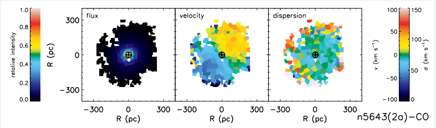
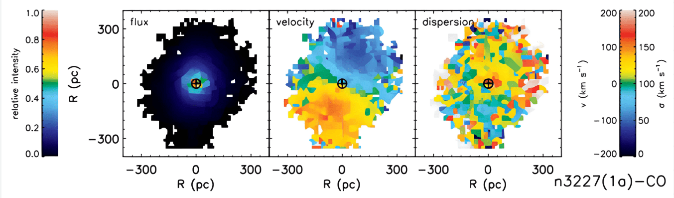
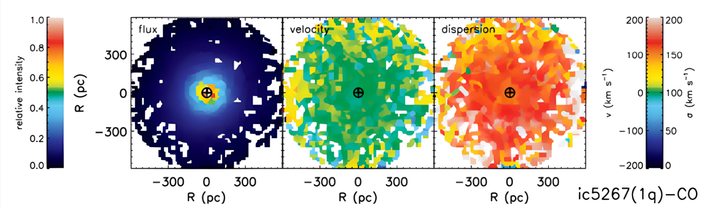
After presenting this table, Hicks et al.⁴ goes on to analyze each galaxy. This analysis allows differences to be easily seen. Each AGN/quiescent galaxy is measured in intensity by flux, velocity, and dispersion. Shown here are the compared 2D maps of CO absorption for a quiescent (no galactic activity), Seyfert 1.5, and Seyfert 2 galaxy.

From the samples in Figures 10 through 12 below, it is clear that in terms of flux, the more active an AGN becomes, the more its flux becomes dense. This is shown by the quiescent galaxy having a relatively spread-out flux with relative intensity to the extent of even 300 parsecs from the galactic nucleus while the more luminous Seyfert 2 galaxy has a much more concentrated flux. This is seen across all three graphs, rather than just the flux graph, and is supported by the figure at the end of Reines et al.² since a more dense AGN correlates with more central luminosity in the innermost kiloparsec, causing a disproportionate ratio between SMBH mass and stellar galactic mass. Another interesting feature is the velocity for both Seyfert galaxies. They both seem to be evenly split with one half being intense and the other relatively less intense. This seems counterintuitive as nuclei proximity normally correlates with galactic intensity which may be an area of future investigation.

Figure 10 | Hicks et al.⁴ – Seyfert 2 NGC 5643

Figure 11 | Hicks et al.⁴ – Seyfert 1.5 NGC 3227

Figure 12 | Hicks et al.⁴ – Quiescent galaxy IC 5267

Overall, Hicks et al.⁴ portrays that the effect of an AGN on a host galaxy is strongly shown in the overall composition of the galaxy. More active or luminous AGN cause an increase in central intensity and a decrease in overall galactic radius.

Discussion

The graph at the end of Reines et al.² suggests that the more massive the AGN, typically, the larger the surrounding galaxy is in terms of stellar mass. This is with the exception of dwarf galaxies which do not seem to follow a line of best fit. Elliptical galaxies tend to have higher mass AGN as well as higher mass host galaxies. This backs up the notion that a more spherical shape is caused by higher mass. Finally, as expected, the paper states that quasar galaxies which have more luminous AGN will have a higher surrounding galactic mass.

McKernan et al.³ suggests that except for some outliers, AGN have a thermal emission limit regardless of mass. It also states that an SMBH’s accretion disk will lead to the creation of IMBH. By extrapolating on this notion, this may be indirect evidence that SMBHs, which all AGN are centered around, are primordial or the result of a massive IMBH merging event. This is also supported by Celotti et al.⁵ which states that massive star death creates stellar mass black holes as opposed to SMBHs.

Hicks et. al⁴ indicates that galactic nucleus activity feeds central SMBH growth, meaning that in the context of the ideas established in the first paper, active galaxies cause overall galaxy growth. Next, they suggest that Seyfert or other AGN typically reside in younger galaxies where there is enough fuel for them to become active. This means that a large amount of primordial AGN have lost their fuel and become quiescent (possibly including our Milky Way). The paper makes the following assertions: Seyfert AGN can feed on stellar fuel within a radius of several kiloparsecs, and quasars are likely caused by galactic mergers. This contradicts the preceding notion of primordial AGN, as Seyfert AGN are known to be less massive than a quasar yet have a gravitational pull strong enough to feed off several kiloparsecs of surrounding material, indicating that a quasar should also have enough gravity to accumulate its mass on its own or with the help of a merger. The figures at the end of Hicks et. al⁴ demonstrates that AGN’s effects on host galaxies are strongly evident in the galaxies’ overall composition. Specifically, more active or luminous AGN contribute to an increase in central intensity and a decrease in overall galactic radius. The relationship between AGN and their host galaxies investigated in these three papers assist in lending context to the subsequent data analysis.

Research Paper

Design & Selection Criteria

In order to determine AGN’s effects on their parent galaxies, the SDSS catalog was used to download the fits files of AGN. Using this catalog, over 35 fits files of “quasar” AGN will be graphed and fitted using Jupyter Notebook. Forty files were chosen specifically for a pragmatic, yet statistically robust analysis. This will help to classify these AGN by plotting their emissions on a BPT diagram. Raw spectra from the Sloan Data Sky Survey (SDSS) Data Release 16 (DR16) were downloaded for analysis. A reference BPT Diagram is plotted below.

Figure 13 | Richardson et al.⁶ – BPT Diagram

Next, quasar-type AGN in a redshift $<$ /= 0.03 z, specifically imported from SDSS, were chosen to focus on AGN that are relatively local in the universe (0.03z $\sim$ 414 million light years) in order to get spectra that are more precise. The specific wavelengths for the hydrogen alpha, hydrogen beta, oxygen III, and nitrogen II were utilized. Below are the given wavelengths of these chemical compounds.

	Hydrogen β	Oxygen III	Nitrogen II	Hydrogen α	Nitrogen II
Wavelength (Å)	4861.333	5006.843	6548.050	6562.819	6583.460

Table 1| Chemical compounds necessary for BPT plotting and their wavelengths, including oxygen III, 2 lines of nitrogen II, hydrogen alpha, and hydrogen beta.

To determine their abundance, flux will be graphed and measured. This can be done with a Jupyter Notebook tutorial on plotting galactic emission lines and producing a fitted curve. A tutorial by Luke Holden, Measuring Emission Line Fluxes with Python⁷, can be utilized to fit the curves and find the measurements. The commonly used threshold for wavelength significance is 3:1 as stated by Iowa State’s Center for Nondestructive Evaluation. So, the amplitude of a wavelength for the above chemical compounds must have a peak of at least 3 times the flux of the surrounding average or “noise.” This would correspond to a signal-to-noise ratio of about 3:1. These measurements are determined by a Gaussian function and will be represented in a normal distribution. In the Gaussian Function below, Equation 3, a is the amplitude of the emission peak, xa is the wavelength of the amplitude, $\sigma$ is the standard deviation of the distribution, x is the wavelength value in lambda, and e represents Euler’s number.

(3) $\begin{equation*}\quad f(x) = a e^{-\frac{(x - x_a)^2}{2\sigma^2}}\end{equation*}$

With this ratio measured, each individual ratio will be compared to the emissions of other chemical compounds and then plotted on the BPT diagram to fit onto the axis shown by Figure 13. By plotting these quasar spectra on the BPT diagrams and measuring their respective chemical abundance, the classification of galaxies from data release 16 of the optical SDSS will be attempted on at least 35 galaxy spectra. This equation is utilized in the code of the above python tutorial. Based on deductions from the literature review about AGN and their characteristics combined with data on the chemical composition of quasar AGN, a general correlation should be able to be made between the qualities of an AGN and the evolution and composition of the host galaxy.

Revisions

AstroimageJ was used to extract flux measurements from the fitz files when the above tutorial proved incompatible with the data. It was also used to extract log-lambda and flux values from the 35 downloaded fitz files off of the SDSS database. AstroimageJ is an extension of ImageJ which provides an astronomy-specific image display environment and tools for astronomy specific image calibration and data reduction. Because of this, it was easily able to interpret the fits files from SDSS. The log-lambda values extracted are the solution to the logarithmic equation below where $\log \lambda$ is given by the AstroimageJ extraction.

(4) $\begin{equation*}f(x) = \log_{10} \lambda = \log \lambda\end{equation*}$

This extraction gave the necessary log lambda and flux measurements for the data analysis. A single example of the measurements is below in Figure 15.

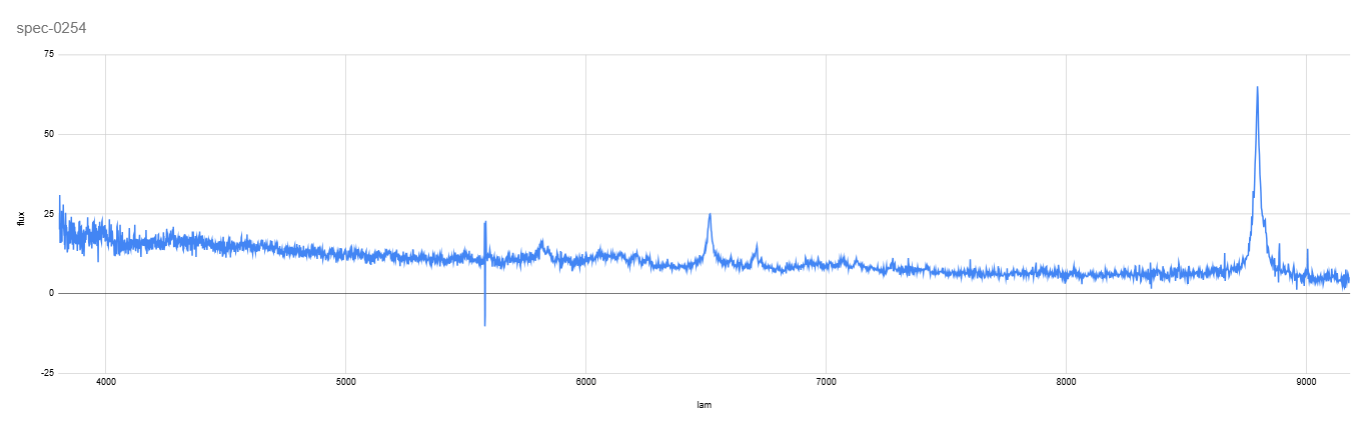
Figure 14 | An example of a measurement and flux given by AstroImageJ (spec-0003) — see Table 1 in the analysis results. AstroImageJ typically produced anywhere between 3835 and 3850 unique $\lambda$ values, each with specific flux variables. Chemical emissions were measured with an error bound of $\pm 50$ from the given wavelengths in Figure 14. This error bound was chosen to fully encompass the emissions of the specific compound. It was selected after examining the graphed spectra and determining the average difference between the two ends of each curve.

Upon obtaining the log lambda values, the actual lambda value could be obtained using exponentiation of the set with a base of 10. It is this lambda vs. flux that is graphed above.

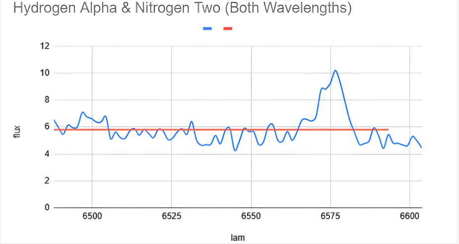
Shown below is an example of a hydrogen alpha/nitrogen II emission which is significant enough to be measured. (Noticeable signal:noise ratios where the signal is the curve amplitude and the noise is the spectral background.)

Figure 15 | Nitrogen II and hydrogen alpha emission curve for spec-0165. See Table 1 in Results. The red line is the flux average in the above data, and the blue line is the actual flux of this spectra.

The emissions for this wavelength can be calculated using an equation with the area between two curves and the Fundamental Theorem of Calculus. Equation 5 below was derived during this data analysis to explicitly measure the emissions of a specific chemical and the signal-to-noise ratio necessary to plot on the BPT Diagram.

(5) $\begin{equation*}\frac{\int_{\lambda(a)}^{\lambda(b)} k\, e^{-\frac{(x-n)^2}{2\sigma^2}} \, dx}{\int_{\lambda(a)}^{\lambda(b)} \mu \, dx}\cdot\frac{S(\text{signal})}{N(\text{Noise})}\end{equation*}$

This equation was utilized to find the signal-to-noise ratio where S(total) represents the total emission of the wavelength, k the amplitude of the Gaussian function (which represents the peak of the emission), h the wavelength at which this peak takes place, and $\sigma$ the standard deviation of the +/- 50 lambda’s corresponding flux values. The lambda bounds are given when the peak curve exceeds the $\mu$ (average) flux value of the specific emission. The $\mu$ is determined by taking the average flux of the surrounding 50 wavelength fluxes on either side in order to remove the possibility of an inaccurate equation due to gradual background noise over a massive amount of lambda values. An example of this is shown below.

Figure 16 | In this example spec 0293 a total $\mu$ value of the entire spectra wouldn’t make sense as the $\mu$ of the entire spectra is likely to be higher than even the peaks at $\lambda$ = 9000

Anticipated Error

Most errors occurring from the usage of these equations are from the approximations used in the input variables. Integrating the total over the base gives a precise measurement for the signal-to-noise ratio. For instance, selecting +/- 50 wavelength for the integration of the emission is an approximate average (+/-) which was taken based on the start and end of the emission across the thirty-five spectra that were graphed. It is probable that curves could start or end at very slightly smaller or higher values than the bounds, however, the bounds cannot be customized to the curve in order to preserve the integrity of the normal distribution equation and its essential symmetry. Every other step in this procedure such as calculating the standard deviation of the values is in the +/- 50 range which may lead to the same type of approximation error.

Finally, the noise ratios vary based on the average flux of the emission. For instance, a low average emission can cause an extremely high ratio as integration is based on the x-axis. In the event of a negative flux average (should not realistically be possible), the equation would fail entirely as there cannot be a negative ratio. (*When referring to average flux of emission, it is the red line in Figure 15.) There is a probability that a negative ratio could occur if the signal is so weak that an offset in the spectra, potentially accounting for background noise from Earth, causes a negative flux.

Method Test

Below is a graph and equation bar of sample spectra, spec-0165, to test the derived equation. (See Table 1 in Results.)

Figure 17 | Visualization of the equation above on the Desmos Graphing Calculator. The scattered points represent the NII and hydrogen alpha emissions of spec-0165. (See Table 1 in Results.) The green and blue lines represent a and b coordinates for integration. These a and b coordinates give an accurate depiction of the emission of the curve, focusing on when the curve exceeds the average/noise of the sample represented by the black line. This figure confirms that the red line given in Equation 3 correctly fits/represents the data.

Figure 18 | Equation tab on Desmos Graphing Calculator for emission measurements. The Gaussian function of the distribution is line 1, the total emission is line 2, and the additional signal minus the background noise is line 3. In this case, line 3 also represents the area between two curves given in Figure 17. These emissions are compared to the flux over the interval in which the emission curve exceeds the sample average within a wavelength +/- 50 lambda. Line 4 is the S/N ratio needed for BPT plotting given by Equation 4. The solution given in line four is the correct signal-to-noise ratio for spec-0165, representing the peak-to-average shown in Figure 16.

This is very much the expected result from a visual standpoint on the graph. This method repeatedly proved successful when measuring abundant emissions. The remaining data was analyzed within these new parameters.

Results

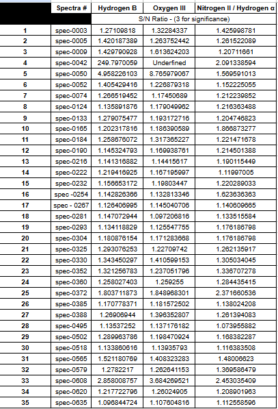
The analyzed sample of AGN spectra consisted of 35 quasar spectra measured with AstroimageJ to analyze their flux and wavelengths. AstroimageJ measured around $\sim$ 3850 wavelength plottable values per quasar spectra. Table 2 below is the documentation of all 35

spectra. All calculation, and emission plots are within +/- 50 lambda of their corresponding wavelengths lambda values given in Figure 14. Hydrogen alpha and Nitrogen II emission measurements were grouped because their approximate wavelengths were within 50 lambda of each other. Below is a table which shows the measured ratios for all 35 samples downloaded from SDSS.

Figure 19 | Each number represents the emission ratio for all 35 spectra. There needs to be a ratio of 3 or more to hold significance.

Conclusion

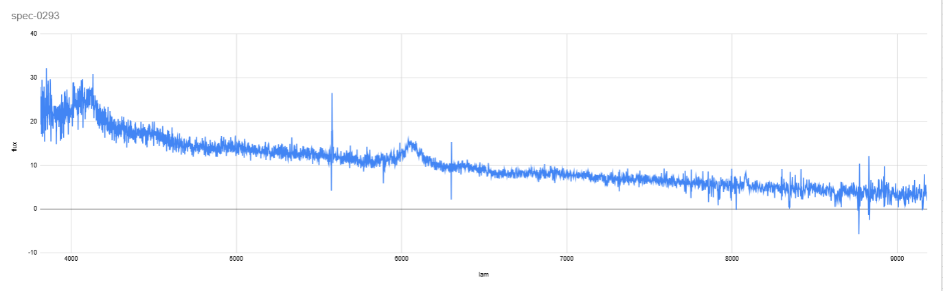
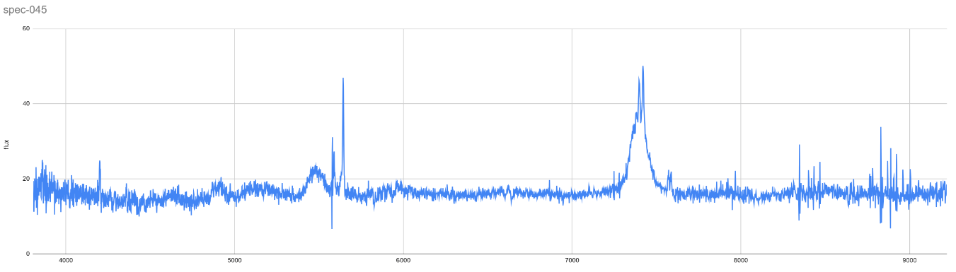
Although several spectra had emissions that were measured, not a single source had the abundance in all four compounds necessary to be plotted on the BPT diagram. However, it is important to note that some emissions did meet the standard for significance. It is also important to acknowledge the errors anticipated in the previous section. For the latter, spec-0042 is an excellent example of a very weak spectra. The average flux for the Oxygen III emission was negative, causing an undefined answer. Similarly, for its Hydrogen Beta emission, there were so many negative values that the average flux neared zero, and the signal ratio ended up being 249 times “larger” than the average despite the lowest (negative) fluxes having an absolute value larger than the amplitude. The measurements from spec-0050 are a similar scenario with the sample +/- 50 lambda containing negative flux values. The Oxygen III emission in spec-0608 was the only emission which met the standard for AGN significance without negative values in its emission. Spec-0372 and spec-0565 also have noticeably higher ratios compared to the others. It is possible that a ratio of three is too high a standard for emission significance or that enough spectra were analyzed. Finally, spectra had emission abundance at other lambda values. The below spectra is an example of an abundance of chemical compounds other than the ones needed for BPT plotting:

Figure 20 | A spectra from the SDSS sample (spec-0495). The massive fluxes between 7000 and 8000 lambda may be grounds for further research as these chemicals may further explain optical characteristics of the specific AGN.

Nevertheless, since none of the sources exhibited all four emission lines – hydrogen alpha, hydrogen beta, nitrogen II, and oxygen III – they could not be plotted on the BPT diagram. Consequently, this limitation prevented drawing conclusive evidence from the data analysis to support the claims discussed. However, examination of these spectra reveals numerous avenues for future research.

Next Steps

Further steps could involve processing more AGN spectral data in order to make the BPT diagram or using an already processed database which holds candidate galaxies with the correct chemical abundance for analysis. For example, rather than using raw data from SDSS, other catalogs such as the MUSE Wide Survey could be utilized which hold AGN spectra that have emission lines with the correct abundance. SDSS was simply used for the opportunity to learn

with raw data. The MUSE Wide Survey could be used as select sources for the BPT diagram. It is a promising database for further analysis. As well, although the intent of the data analysis was unfulfilled by the lack of specific chemical abundance, the 35 AGN spectra plotted in Table 1 seemed to have an abundance in other wavelengths. This could serve as a breadcrumb for a future analysis.

Acknowledgements

First, I would like to thank my father and mother who supported this research opportunity. Secondly, I would like to thank my mentor, Dr. Marziye Jafariyazani, who did an excellent job in helping me understand material from various textbooks to prepare for the writing of this paper. Dr. Jafariyazani never failed to make difficult material easy, and she guided me through the conceptualization, formatting, and referencing for this paper. I would also like to thank her for the opportunity I had to analyze data with Python. I am grateful to AstroImageJ, Jupyter Notebooks, Google Suite, and YouTube programming tutorials for their incredible open source platforms.

I would also like to extend my appreciation to my teachers at Nashua High School South, including Mr. Jeffrey Durnford from AP Statistics, Ms. Kellie Gabriel from AP Calculus, and Mr. Anthony Spero from AP Computer Science, who helped me troubleshoot the mathematics and technical errors with the software. I would like to thank Lumiere Education who provided me with the opportunity to work with a researcher in my desired sector of astronomy. The Lumiere program assisted in editing the scientific writing, preparing for publication, and adhering to a timeline. As a senior in high school, I am grateful to have worked on AGN at my stage of learning, and I look forward to further research in the fields of astronomy, astrophysics, and mathematics during undergraduate studies, graduate school, and in my future career.

As a high school student, it was a privilege to undertake this project. Coming into this, I hoped to learn more about working with black holes and the genesis of galaxies. I had previously worked with exoplanets and their lightcurves and transits, but this paper delved more into the physics of astronomical phenomena in which I am keenly interested. Outside of astronomy, I learned more about the scientific method and the expertise needed to write a scholarly paper. Through this experience, I learned that hypotheses do not always end in hoped for results, that failure is a necessary part of scientific inquiry, and that resilience is key to finding alternative solutions. Regardless of what comes next, the insight I gained from this paper will be invaluable to my future research in astrophysics.

References

An Introduction to Active Galaxies. The Open University; 2016 [↩] [↩] [↩] [↩] [↩]
Reines A.E., Volonteri M., 2015, ApJ, 813, 82. doi:10.1088/0004-637X/813/2/82 [↩] [↩] [↩] [↩] [↩] [↩] [↩] [↩] [↩] [↩] [↩] [↩] [↩] [↩] [↩]
McKernan B., Ford K.E.S., Kocsis B., Lyra W., Winter L.M., 2014, MNRAS, 441, 900. doi:10.1093/mnras/stu553 [↩] [↩] [↩] [↩] [↩]
Hicks E.K.S., Davies R.I., Maciejewski W., Emsellem E., Malkan M.A., Dumas G., Muller-Sanchez F., et al., 2013, ApJ, 768, 107. doi:10.1088/0004-637X/768/2/107 [↩] [↩] [↩] [↩] [↩] [↩] [↩] [↩] [↩] [↩] [↩] [↩] [↩] [↩]
Celotti et. al 1999, Astrophysical evidence for the existence of black holes. doi:10.1088/0264-9381/16/12A/301 [↩]
Richardson, Chris & Allen, James & Baldwin, Jack & Hewett, Paul & Ferland, G.. (2013). Interpreting the Ionization Sequence in AGN Emission-Line Spectra. Monthly Notices of the Royal Astronomical Society. 437. 10.1093/mnras/stt2056. [↩]
Holden, Luke. “Tutorial – Measuring Emission Line Fluxes with Python and Deriving Gas Properties.” Measuring Emission Line Fluxes with Python – Tutorial, Luke Holden, 30 Jan. 2023, lukeholden.com/blog/measuring_emission_line_fluxes_python.html. [↩]

Investigating the Effect of Active Galactic Nuclei on Their Host Galaxies

Abstract