Evaluating Medical Imaging Techniques and AI Models Using Transfer Learning for MRI-Based Brain Tumor Classification

Abstract

Brain tumors pose a serious health risk and are commonly diagnosed using non-invasive imaging techniques such as Computed Tomography (CT) machines, Magnetic Resolution (MRI) machines, Positron Emission Tomography (PET) scans, and ultrasound. This study explores the use of artificial intelligence to classify MRI images into four categories: glioma, meningioma, pituitary tumor, and no tumor. Three machine learning (ML) models (Artificial Intelligence (AI)  models that detect patterns and differentiate data set images into multiple groups)— Convolutional Neural Network (CNN), EfficientNet, and Vision Transformer (ViT) —were fine-tuned using transfer learning. Among them, ViT achieved the highest classification accuracy of 72.34%, demonstrating the potential of transformer-based models in medical image analysis.

Keywords: CT, Machine Learning (ML), Deep Learning, Vision model, CNN

1. Introduction

Brain tumors are a severe medical condition requiring accurate diagnosis through non-invasive imaging techniques. These methods allow doctors to examine the brain without surgical intervention, helping to identify and classify tumors effectively. Various imaging modalities are commonly used, including CT, ultrasound, and MRI, each employing different principles. CT scans utilize ionizing radiation, which can be harmful due to its potential to alter cellular DNA, increasing the risk of tumor recurrence^1,2. Ultrasound relies on sound waves to create images but is less commonly used for brain imaging due to its lower resolution³. MRI, on the other hand, uses strong magnetic fields, making it a preferred diagnostic tool as it does not expose patients to radiation, thus reducing health risks⁴. Despite its advantages, MRI has limitations. Patients with metal implants cannot undergo MRI scans due to the strong magnetic fields interfering with metal-containing medical devices⁵. However, MRI remains a highly effective imaging technique due to its high-resolution imaging capabilities and non-invasive nature, making it the preferred method for diagnosing brain tumors⁶. After acquiring MRI images, doctors must classify them to accurately diagnose the type of brain tumor present. Traditional diagnostic methods rely on expert interpretation, but recent advancements in AI and ML have revolutionized medical imaging⁷. ML algorithms can analyze and categorize medical images by identifying subtle patterns that may not be easily detected by the human eye. In this study, MRI images were analyzed using three different deep learning models: CNN, EfficientNet, and ViT. CNN is a foundational deep-learning model widely used for image classification tasks due to its ability to learn hierarchical spatial features through convolutional operations⁸. EfficientNet improves classification accuracy by optimizing model scaling using compound coefficients.ViT, a deep learning model, classifies images by dividing them into patches and analyzing their relationships, often achieving high accuracy⁹. To evaluate their performance, MRI images were split into two datasets: 88% for training and 12% for testing but the imbalance can be fixed through the use of Synthetic Minority Oversampling Technique. The dataset was sourced from Kaggle using KaggleHub and in this study, we comparatively evaluate the performance of several state-of-the- art image classification models using standard accuracy metrics to identify the model that performs best on the selected dataset.

2. Literature Review

Medical imaging plays a foundational role in the non-invasive diagnosis of brain tumors. Among the available modalities, Computed Tomography (CT) and Magnetic Resonance Imaging (MRI) are the most widely used. CT scans, while fast and accessible, rely on ionizing radiation, which has been linked to increased long-term cancer risk, particularly in pediatric populations¹⁰. MRI, by contrast, utilizes strong magnetic fields and radio waves to produce detailed anatomical images without the risks associated with radiation exposure, making it the preferred choice in many clinical scenarios¹¹. However, limitations exist—MRI cannot be performed on patients with metal implants or certain medical devices, necessitating clinical discretion in imaging selection¹².

Parallel to advances in imaging, artificial intelligence—particularly machine learning (ML) and deep learning (DL) models—has emerged as a powerful tool for automated image classification. Traditional Convolutional Neural Networks (CNNs), introduced by Krizhevsky et al. (2017), extract hierarchical spatial features and have proven effective across numerous medical imaging tasks. More recently, EfficientNet, a family of models that optimize depth, width, and resolution simultaneously through compound scaling, has demonstrated improved performance in image classification tasks while maintaining computational efficiency¹³. Meanwhile, Vision Transformers (ViT), which leverage self-attention mechanisms across image patches, have shown strong performance in capturing global contextual relationships, a feature especially useful in high-resolution medical imagery¹⁴.

The integration of these models into brain tumor classification tasks is a growing area of research, with studies demonstrating their utility in differentiating between gliomas, meningiomas, pituitary tumors, and normal brain tissue. This study builds on these developments by conducting a comparative evaluation of CNN, EfficientNet, and ViT architectures applied to a curated MRI dataset. By doing so, it seeks to identify which architecture offers the most clinically relevant accuracy, with a long-term view toward augmenting diagnostic workflows in neuro-oncology.

3. Methods

Information regarding the paper is sourced from scholarly articles from reputed journals such as: ScienceDirect, PubMed, and others. The learning process was initiated by understanding if cancer is caused by CT machines^15,16, and knowledge about other scanning machines such as MRI, Ultrasound and PET was gradually acquired. There was still focus on how CT could cause cancer through the use of ionized radiation, while also research on the pros and cons of each machine began^17,18. The use of ionized radiation by CT was shown to be a legitimate concern for cancer¹⁹. Insights into these medical machines were gained by examining their pros and cons, which facilitated an understanding of the circumstances in which the use of each machine would be optimal. The structure of the brain, including the meninges and other parts of the nervous system, was also studied²⁰. This contributed to an understanding of tumor classification. Additionally, data were analyzed to determine when certain medical machines were preferred over others by understanding the structure of the nervous system and the pros and cons of each machine. For example, MRI machines are generally preferred over CT machines because they are considered safer due to not using ionized radiation; however, in circumstances involving a patient with metal in their head, a CT scan must be employed²¹. A CT scan would need to be utilized due to the potential dangers posed by the magnetism of MRI machines for such patients. Furthermore, the understanding of brain structure aids in deciding which technique should be employed. If a tumor is located in a critical area of the brain that may control vision, hearing, or other essential life functions, options for tumor removal are ruled out. Consequently, techniques like biopsies are not utilized, as they can cause permanent damage to these vital functions. Also, sex, age, and race matter during choosing a radiological machine because, for example, these factors can influence the likelihood of getting cancer from the ionizing radiation used in CT machines²². MRI machines are known to be very expensive, meaning that a doctor’s facility may not have access to one. This could limit the available options to other scans like CT or PET scans. At times, a specific method may be ruled out, as the least intrusive option is typically preferred by doctors; for example, a brain surgery would not be performed solely for a biopsy when an MRI or CT scan could be conducted instead. Also, different images of varying tumors were compared using a CNN system on CT scans. CNN, a type of ML that utilizes repeated knowledge inputs to learn a specific action to a high level. It utilizes many ways to correct its computing errors – resets each of its layers by altering the weights – until it can correctly distribute the data. This allows easier distribution of the tumor images into different categories of no tumors, meningioma tumors, glioma tumors, and pit tumors. 

The process of setting up and analyzing each ML model is as shown in the points below.

After researching the different radiological machines, it was clear that MRIs were the safest among all the radiological machines due to their nature of being noninvasive while still having a clear resolution. MRIs also do not use ionized radiation which lowers the risk of danger to patients. The biggest problem for MRI was that it uses magnetism which can pose problems for patients who have metal implants. The MRI images were then put through CNN, ViT, Efficient-Net data systems.

1. Data Collection and Preprocessing

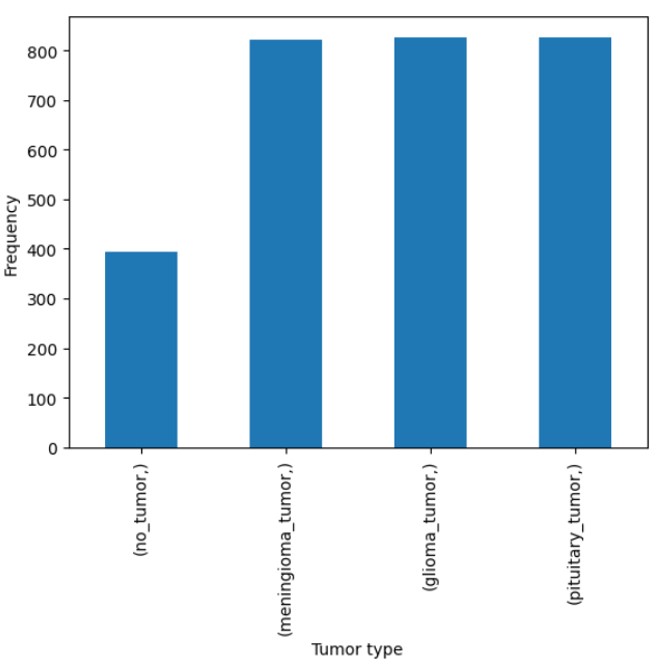
Figure 10 provides an overview of the flowchart, illustrating the step-by-step process of our methodology. The dataset used in this study was sourced from Bhuvaji et. al’s kaggle²¹ data set. The data consisted of high-resolution images categorized into multiple classes. For preprocessing, all images were resized to a uniform size of 224×224×3 to ensure compatibility with the input requirements of the models. The class labels were encoded into numerical values using the LabelEncoder function from the scikit-learn library, standardizing the categorical target variable for model training. The encoded labels were then used to transform both the training and testing datasets. Figure 8 shows the number of images used in each tumor category for the training phase, while Figure 9 shows the number of images used in each tumor category for the testing phase. This preprocessing pipeline ensured a consistent data format and dimensionality, facilitating effective learning by the models while maintaining the integrity of the original dataset. After preprocessing, the training dataset comprised 2870 samples, and the testing dataset included 394 samples. All images in the data set were used and due to this, there was no use of a sampling method to ensure representativeness. Since all the data that was being offered was used, one can classify it as a census which is more representative of the population than any other sampling method.

2. CNN Model Architecture

The CNN architecture used in this study is a sequential model designed for the multi-class classification of MRI images. The model begins with a convolutional layer comprising 8 filters with a kernel size of 5×5 and rectified linear unit (ReLU) activation, which extracts spatial features from the input images of size 224 x 224 x 3. To ensure consistency and align with established practices, we adopted the input resolution of 224×224 pixels, as used in prior work. Specifically, we followed the precedent set by: S. Tummala, S. Kadry, S. A. C. Bukhari, H. T. Rauf. Classification of brain tumor from magnetic resonance imaging using vision transformers ensembling. Current Oncology, 29, 7498–7511 (2022). This is followed by a max-pooling layer with a pool size of 5×5, which reduces spatial dimensions and mitigates overfitting. The feature extraction process continues with two additional convolutional layers, each with 8 filters and kernel sizes of 3×3, both employing ReLU activation for non-linear transformation. These are followed by corresponding max-pooling layers with pool sizes of 3×3 and 2×2, respectively, for progressive down-sampling of feature maps. After the convolutional and pooling layers, the model transitions into a fully connected architecture with a flattening layer, which transforms the extracted feature maps into a one-dimensional vector. This is followed by a dense layer with 128 neurons and ReLU activation, which serves as a high-level feature representation. Regularization is incorporated using a dropout layer with a 20% dropout rate to prevent overfitting. Subsequently, two additional dense layers with 64 and 32 neurons, respectively, both employing ReLU activation, further refine the extracted features. Each dense layer is followed by a dropout layer with a 20% dropout rate to enhance generalization. The final dense layer consists of 4 neurons, corresponding to the four tumor classes (glioma, meningioma, pituitary, and no tumor), and utilizes a softmax activation function to output class probabilities. This architecture is designed to balance complexity and computational efficiency, making it suitable for the classification of medical imaging datasets with limited variability.

3.  Efficient-Net Model Architecture

The EfficientNet-based model utilized in this study builds upon the EfficientNetV2B3 architecture, a member of the EfficientNet family of CNNs renowned for its state-of-the-art accuracy and computational efficiency in image recognition tasks. EfficientNet employs a novel compound scaling method to systematically balance model depth, width, and resolution, optimizing performance under various resource constraints. Derived from a baseline architecture (EfficientNet-B0) through neural architecture search, the EfficientNet family scales up to larger models (EfficientNet-B7), offering versatility for diverse applications. In this work, the EfficientNetV2B3 model, pre-trained on ImageNet, is used as a feature extractor. The top layers of the base model were excluded, and a lightweight classification head was added, consisting of a global average pooling layer followed by a fully connected dense layer with softmax activation for multi-class classification. This design leverages the pre-trained model’s robust feature extraction capabilities while maintaining computational efficiency, making it well-suited for domain-specific fine-tuning in computer vision tasks¹². Point 14: batch_size = 32 n_epochs = 15 alpha = 0.01 Efficient net Total params: 12936770 (49.35 MB) Trainable params: 12827554 (48.93 MB) Non-trainable params: 109216 (426.62 KB)

4. ViT Model Architecture:

The ViT-based model employed in this study is built upon the ViT-B32 architecture, which is part of the pioneering family of transformer-based models for image recognition. Unlike traditional CNN models, ViT processes images as sequences of patches, enabling it to capture long-range dependencies and global context effectively. Due to the data set being pre trained with certain sized data sets, we only had a small data set size to use for the ViT. The pre-trained ViT-B32 model, initialized with weights optimized for image classification tasks, serves as the base feature extractor. To adapt this architecture to the specific classification task, additional layers were appended, including a flattening layer, batch normalization layers to stabilize and accelerate training, and a dense layer with Gaussian Error Linear Unit (GELU) activation to introduce non-linearity. The final layer is a dense layer with softmax activation, designed to output class probabilities. This configuration harnesses the transformer architecture’s strength in feature representation while tailoring it for the multi-class classification task, ensuring high accuracy and robust performance²³.

5. Training Procedure

The training procedure was designed for a multi-class classification task involving 4 classes (glioma tumor, meningioma tumor, no tumor, and pituitary tumor) corresponding to the labels: glioma tumor, meningioma tumor, no tumor, and pituitary tumor. The dataset consisted of images resized to a uniform dimension of 224×224×3 to meet the input requirements of the model. The model was trained using a batch size of 32 over 15 epochs, ensuring adequate iterations for effective learning. A validation split of 20% was employed, reserving part of the training data for validation to monitor the model’s performance and prevent overfitting. The Adadelta optimizer with a learning rate of α=0.01 was used to adaptively adjust the learning rate during training. The loss function, sparse_categorical_crossentropy, was utilized to handle the integer-encoded multi-class labels efficiently. This well-structured training pipeline enabled the model to classify images across the four tumor categories accurately.

4. Results

Evaluation Criteria

The evaluation of the model’s performance was conducted using several key metrics. First, precision, recall, and F1-score were calculated using the precision_score, recall_score, and f1_score functions, respectively, with the ‘macro’ average method. These metrics provide insights into the model’s ability to correctly classify instances from each class, accounting for both FP and false negatives (FN). Additionally, a confusion matrix was generated to visually assess the classification performance across all classes. This was plotted using the ConfusionMatrixDisplay to identify misclassifications and the overall distribution of predictions. To further evaluate the model’s ability to discriminate between classes, the ROC curve and AUC were plotted for each class using the plot_roc_curve function. The ROC curve provides a graphical representation of the trade-off between the true positive (TP) rate and FP rate, and the AUC value quantifies the model’s ability to correctly classify instances. These metrics and visualizations collectively offered a comprehensive evaluation of the model’s performance in the multi-class classification task. The three models—CNN, EfficientNet, and ViT—were compared using the same set of evaluation metrics to ensure a fair and consistent performance analysis.

●   Precision: Precision is the ratio of correctly predicted positive observations to the total predicted positive observations. It reflects how many of the predicted positive cases are actually positive. A higher precision means fewer FPs.
Equation #1: Precision=TP/TP+FP
where TP is the number of true positives, and FP is the number of false positives.

●   Recall: Recall (also known as Sensitivity or TP Rate) is the ratio of correctly predicted positive observations to all observations in the actual class. It shows how many of the actual positive cases were correctly identified by the model. A higher recall means fewer FN.
Equation #2: Recall=TP/TP+FN
where TP is the number of true positives, and FN is the number of false negatives.

●   F1-Score: The F1-score is the harmonic mean of precision and recall. It combines both metrics into a single value that balances the trade-off between them, especially when there is an uneven class distribution (imbalanced dataset). A higher F1-score indicates a better balance between precision and recall.
Equation #3: F1-Score=2×(Precision×Recall/Precision+Recall)

●   Confusion Matrix: A confusion matrix is a table used to evaluate the performance of a classification algorithm. It summarizes the number of correct and incorrect predictions for each class in a matrix format. The matrix contains:

●   True Positive (TP): Correctly predicted positive class.

●   True Negative (TN): Correctly predicted negative class.

●   False Positive (FP): Incorrectly predicted as positive class.

●   False Negative (FN): Incorrectly predicted as negative class.

The confusion matrix helps in identifying the types of errors made by the classifier and is the foundation for calculating other metrics like precision, recall, and F1-score.

●   ROC Curve: The ROC curve is a graphical representation of the performance of a binary classification model at various threshold settings. It plots the TP Rate (Recall) against the Equation #4: FP Rate (1 – Specificity). The ROC curve helps to visualize the trade-offs between sensitivity and specificity across different decision thresholds, providing a clear overview of the model’s discrimination ability.

●   AUC: The AUC is a scalar value that quantifies the overall ability of the model to discriminate between positive and negative classes. An AUC of 1 indicates perfect classification, while an AUC of 0.5 indicates random guessing. A higher AUC indicates better model performance, as it signifies that the model is better at distinguishing between the classes.

Analysis

This study evaluates the performance of three deep learning models—EfficientNet, CNN, and ViT—for multi-class tumor classification. The models were assessed using confusion matrices, receiver operating characteristic (ROC) curves, and quantitative metrics, including precision, recall, F1-score, and accuracy.

Confusion Matrix Analysis

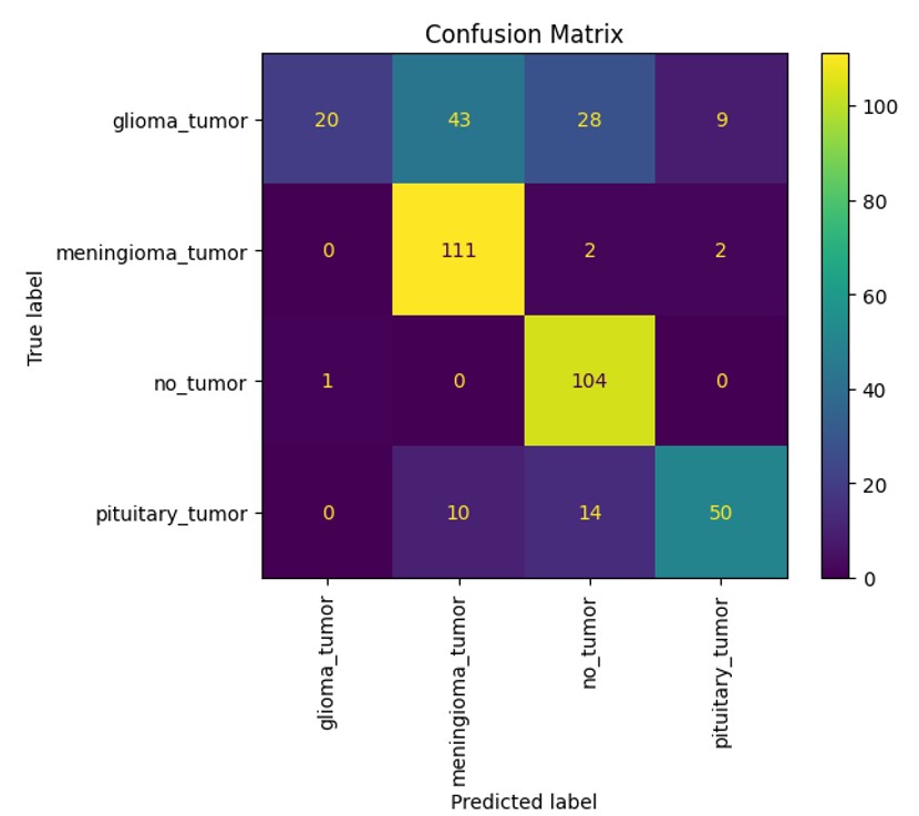
The confusion matrices (Figures 1–3) reveal the distribution of correct and incorrect predictions across the four tumor classes: glioma tumor, meningioma tumor, no tumor, and pituitary tumor. EfficientNet demonstrated relatively balanced performance but showed misclassifications, particularly for glioma and pituitary tumors. ViT exhibited improved classification accuracy across all tumor classes, with significantly fewer misclassifications in the no tumor and meningioma tumor categories. CNN, on the other hand, displayed the highest rate of misclassification, particularly for glioma tumors, which were often confused with pituitary tumors and meningioma tumors.

Explanation of how each deep learning model performed on the different types of tumor images:

EfficientNet performed well in classifying meningioma tumors and no tumors with it having gotten 80 of meningioma tumors correctly classified and 98 no tumors correctly classified. It was not as successful with the other types with only around 30 in both being correctly classified. With ViT, it was able to correctly get 111 meningioma tumors correctly classified along with 104 no tumors correctly classified. It did not do as well in the other categories with only 20 gliomas tumors correctly classified and 50 pituitary tumors correctly classified. Finally, CNN got 90 meningioma tumors correctly classified and 101 no tumors correctly classified. It had lower performances with the other categories with 17 glioma tumors correctly classified and 25 pituitary tumors correctly classified. With all the deep learning models, it was apparent that meningiomas tumor and no tumor images were more commonly correctly classified than glioma and pituitary tumor images.  

ROC Curves

The ROC curves (Figures 4–6) illustrate the models’ ability to distinguish between classes. ViT achieved the highest area under the curve (AUC) values across all classes, with an AUC of 0.77 for glioma tumor, 0.92 for meningioma tumor, 0.99 for no tumor, and 0.92 for pituitary tumor. EfficientNet also performed well, with AUC values of 0.76, 0.93, 0.98, and 0.97 for the respective classes. CNN lagged behind, particularly for the glioma tumor class, with an AUC of 0.54.

Quantitative Metrics

The quantitative evaluation of the models is summarized in Table 1. ViT achieved the highest overall accuracy (72.34%) and F1-score (0.672), demonstrating superior performance compared to EfficientNet and CNN. We would like to clarify several key differences between our study and that of Tummala et al., which contribute to the observed variance in performance. Dataset differences within Tummala et al.’s study is due to the fact that Tummala et al.’s utilized a dataset comprising 3,064 T1-weighted contrast-enhanced MRI slices sourced from Figshare, focusing on three tumor types: meningiomas, gliomas, and pituitary tumors. In contrast, our study employed a different publicly available dataset, which, while similar in nature, differs in size, imaging techniques and class distribution. These differences inherently affect model performance and limit direct comparability. EfficientNet followed with an accuracy of 65.23% and an F1-score of 0.611. CNN achieved the lowest performance metrics, with an accuracy of 59.13% and an F1-score of 0.530. Precision and recall values were consistent with these trends, with ViT achieving the highest precision (0.787) and recall (0.707).

Model Name	Precision	Recall	F1	Accuracy
EfficientNet	0.785	0.625	0.611	0.652
ViT	0.787	0.707	0.672	0.723
CNN	0.673	0.563	0.530	0.591

ViT emerged as the most robust model for multi-class tumor classification, achieving the highest accuracy, F1-score, and AUC values across most tumor classes. EfficientNet performed moderately well, demonstrating better generalization than CNN but underperforming compared to ViT. CNN’s lower performance, as reflected in all metrics, highlights its limitations for this specific classification task.

Loss Curves

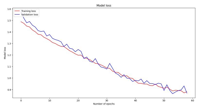
Loss curves are fundamental diagnostic tools in deep learning that visualize the training and validation loss over epochs, providing critical insights into model convergence behavior and generalization performance. The training loss represents how well the model fits the training data, while the validation loss indicates the model’s ability to generalize to unseen data. Ideally, both curves should decrease monotonically and converge to similar values, indicating good model performance without overfitting. A widening gap between training and validation loss suggests overfitting, where the model memorizes training data but fails to generalize. In our comparative analysis, the CNN model exhibited typical deep learning convergence patterns with both losses decreasing steadily until plateauing around epoch 25, demonstrating stable learning dynamics. The Vision Transformer (ViT) showed the smoothest and most consistent convergence behavior with both training and validation losses following nearly parallel downward trajectories throughout training, indicating well-balanced learning dynamics and effective generalization. The EfficientNet model demonstrated rapid initial convergence with steep loss reduction in the first 20 epochs, followed by more gradual improvement, characteristic of efficient architectures that quickly learn dominant features before fine-tuning, ultimately achieving competitive final loss values.

Training and validation loss curves for the Vision Transformer (ViT) model over 60 epochs. The model exhibits   the smoothest convergence behavior with both training and validation losses following consistent downward trajectories, demonstrating well-balanced learning dynamics and effective generalization capabilities.

Training and validation loss curves for the EfficientNet model over 60 epochs. The model demonstrates rapid initial convergence with steep loss reduction in the first 20 epochs, followed by more gradual improvement, characteristic of efficient architectures that quickly capture dominant features before fine-tuning for optimal performance.

5. Discussion

This study explored the use of ML models to classify brain tumors using MRI imaging data into four categories—glioma, meningioma, pituitary tumors, and no tumor. The study focuses on the classification of different tumor images by different ML models. MRI machines were chosen as they are generally safe due to not using ionized radiation. A downside of MRI scans is that they cannot be used if the patient has metal in their bodies²⁴. MRIs also have high resolution while still having a non-invasive nature, meaning that the images produced by MRIs are very clear and are easier to classify. The study employed three ML models—EfficientNet, CNN, and ViT—to see which model classified the MRI images the most accurately. The possibilities of the models can help the classification of radiological machines become automated²⁵.  The models’ performance was assessed using confusion matrices, ROC curves, and metrics such as precision, recall, F1-score, and accuracy. Among these, ViT emerged as the most robust model, achieving the highest overall accuracy (72.34%), precision (0.787), recall (0.707), and F1-score (0.672). EfficientNet demonstrated moderate performance, while CNN lagged behind in all metrics. These findings align with the growing recognition of the potential of advanced deep learning models like ViT for medical image analysis. Precision and recall metrics are particularly critical in the context of medical datasets. High precision metric ensures that when a model predicts the presence of a tumor, the prediction is reliable, reducing the risk of false positives (FP) that could lead to unnecessary treatments and patient anxiety. On the other hand, recall metric measures the model’s ability to identify all actual tumor cases, minimizing the risk of giving a patient a wrong treatment or not giving a treatment when necessary.

References

1. D. J. Brenner, R. Doll, D. T. Goodhead, E. J. Hall, C. E. Land, J. B. Little, J. H. Lubin, D. L. Preston, R. J. Preston, J. S. Puskin, E. Ron, R. K. Sachs, J. M. Samet, R. B. Setlow, M. Zeider, Cancer risks attributable to low doses of ionizing radiation: assessing what we really know. Proceedings of the National Academy of Sciences, 100, 13761-13766 (2003). [↩]
2. S. Hussain, I. Mubeen, N. Ullah, S. S. U. D. Shah, B. A. Khan, M. Zahoor, R. Ullah, F. A. Khan, M. A. Sultan. Modern diagnostic imaging technique applications and risk factors in the medical field: a review. NIH, 2022, 1-19 (2022). [↩]
3. E. Mace, G. Montaldo, B. O. Osmanski, I. Cohen, M. Fink, M. Tanter. Functional ultrasound imaging of the brain: theory and basic principles. Far East NDT New Technology & Application Forum, 60, 492-506 (2013). [↩]
4. M. Carr, M. L. Grey. Magnetic resonance imaging overview, risks, and safety measures. AJN, 102, 26-33 (2002). [↩]
5. M. F. Dempsey, B. Condon, D. M. Hadley. MRI safety review. ScienceDirect, 23, 392-401 (2002). [↩]
6. M. Martucci, R. Russo, F. Schimperna, G. D’Apolito, M. Panfili, A. Grimaldi, A. Perna, A. M. Ferranti, G. Varcasia, C. Giordano, S. Gaudino. Magnetic resonance imaging of primary adult brain tumors: state of the art and future perspectives. biomedicines, 11, 364, (2023). [↩]
7. X. Li, L. Zhang, J. Yang, F. Teng. Role of artificial intelligence in medical image analysis: a review of current trends and future directions. Journal of Medical and Biological Engineering, 44, 231-243 (2024). [↩]
8. A. Krizhevsky, I. Sutskever, G. E. Hinton. ImageNet classification with deep convolutional neural networks. Communications of the ACM, 60, 84-90 (2017). [↩]
9. Dosovitskiy, A.; Beyer, L.; Kolesnikov, A.; Weissenborn, D.; Zhai, X.; Unterthiner, T.; Dehghani, M.; Minderer, M.; Heigold, G.; Gelly, S.; et al. An Image is Worth 16 × 16 Words: Transformers for Image Recognition at Scale. arXiv 2020, arXiv:2010.11929 [↩]
10. Hauptmann et al., 2023; Lin, 2010 [↩]
11. Martucci et al., 2023 [↩]
12. Dempsey et al., 2002 [↩]
13. Tan & Le, 2019 [↩]
14. Dosovitskiy et al., 2020 [↩]
15. M. Hauptmann, G. Byrnes, E. Cardis, M. O. Bernier, M. Blettner, J. Dabin, H. Engels, T. S. Istad, C. Johansen, M. Kaijser, K. Kjaerheim, N. Journy, J. M. Meulepas, M. Moissonnier, C. Ronckers, I. Thierry-Chef, L. L. Cornet, A. Jahnen, R. Pokora, M. B. de Basea, J. Figuerola, C. Maccia, A. Nordenskjold, R. W. Harbron, C. Lee, S. L. Simon, A. B. de Gonzalez, J. Schüz, A. Kesminiene. Brain cancer after radiation exposure from CT examinations of children and young adults: results from the EPI-CT cohort study. The Lancet Oncology, 24, 45-53 (2023). [↩]
16. E. G. Stein, L. B. Haramati, E. Bellin, L. Ashton, G. Mitsopoulos, A Schoenfeld, E. J. Amis Jr. Radiation exposure from medical imaging in patients with chronic and recurrent conditions. Journal of the American College of Radiology, 7, 351-359 (2010). [↩]
17. E. Picano, E. Vano, L. Domenici, M. Bottai, I. Thierry-Chef. Cancer and non-cancer brain and eye effects of chronic low-dose ionizing radiation exposure. BMC Cancer, 12, 157 (2012). [↩]
18. M. Z. Braganza, C. M. Kitahara, A.B. de Gonzáles, P. D. Inskip, K. J. Johnson, P. Rajaraman. Ionizing radiation and the risk of brain and central nervous system tumors: a systematic review. Neuro-Oncology, 14, 1316-1324 (2012). [↩]
19. E. C. Lin. Radiation risk From medical imaging. Mayo Clinic Proceedings, 85, 1142-1146 (2010). [↩]
20. C. M. Kitahara, M. S. Linet, S. Balter, D. L. Miller,  P. Rajaraman, E. K. Cahoon, R. Velazquez-Kronen, S. L. Simon, M. P. Little, M. M. Doody, B. H. Alexander, D. L. Preston. Occupational radiation exposure and deaths from malignant intracranial neoplasms of the brain and CNS in U.S. radiologic technologists. American Journal of Roentgenology, 208, 1278-1284 (2017). [↩]
21. T. Seute, P. Leffers, G. P. M. ten Velde, A. Twijnstra. Detection of brain metastases from small cell lung cancer. Cancer, 112, 1827-1834 (2008). [↩]
22. M. Katsuru, J. Sato, M. Akahane, T. Furuta, H. Mori, O. Abe. Recognizing radiation-induced changes in the central nervous system: where to look and what to look for. RadioGraphics, 41, 224-248 (2021). [↩]
23. S. Tummala, S. Kadry, S. A. C. Bukhari, H. T. Rauf. Classification of brain tumor from magnetic resonance imaging using vision transformers ensembling. Current Oncology, 29, 7498-7511 (2022). [↩]
24. R. Kaifi. A review of recent advances in brain tumor diagnosis based on AI-based classification. PubMed, 18, 1-32 (2023). [↩]
25. M. Tan, Q. V. Le. EfficientNet: rethinking model scaling for convolutional neural networks. ICML, 2019, 1-11 (2019). [↩]