Deep Learning Framework for Kidney Tumor Segmentation with Surgical Method Recommendation and Operative Time Prediction

December 14, 2025

422

Abstract

Kidney cancer poses major challenges in diagnosis and surgical management, requiring precise tumor assessment to guide treatment. This study introduces a two-stage deep learning framework designed to support personalized surgical planning. In the first stage, a segmentation model accurately delineates kidney tumors from CT images, enabling precise identification of tumor boundaries critical for planning. The second stage integrates imaging features derived from the segmented tumors with patient clinical data, such as age, body mass index, and tumor size, to recommend optimal surgical strategies and predict operative time. By combining radiological imaging with relevant clinical information, the framework provides tailored surgical guidance that considers both anatomical and patient-specific factors. This multimodal approach allows for more accurate, data-driven decision-making that can adapt to each patient’s unique condition. The model demonstrates strong potential for improving preoperative planning by offering efficient and personalized recommendations, which may lead to better surgical outcomes and resource utilization. Additionally, this study highlights the importance of integrating diverse data sources in medical AI development to capture the complexity of kidney tumors and surgical contexts. The results underscore the value of deep learning in enhancing surgical assistance by bridging imaging data with clinical insights, ultimately contributing to advancements in precision medicine and patient-centered care. This framework represents a promising step towards AI-enabled kidney cancer surgery planning that supports clinicians in making informed, patient-specific treatment decisions.

Introduction

The kidney serves as the body’s primary regulator of homeostasis, maintaining stable fluid balance and plasma volume despite fluctuations in diet, environment, or physical stress across individuals and over time. By precisely managing the retention and elimination of water and electrolytes, the kidney controls the composition of both intracellular and extracellular fluids. It also removes nitrogenous waste from metabolism and clears pharmacologic and toxic substances¹. Beyond waste elimination, the kidneys are essential for regulating blood pressure, producing red blood cells, and managing bone and mineral metabolism. Given their crucial role in maintaining systemic homeostasis, any pathological changes in the kidneys, including neoplasms, can have profound consequences for overall health.

Kidney cancer is an increasingly prevalent malignancy that poses significant diagnostic and therapeutic challenges in clinical practice. As one of the top ten most common cancers worldwide, it accounts for a substantial proportion of global cancer-related morbidity and mortality. In 2008, 54,390 Americans were diagnosed with kidney cancer and 13,010 died; Renal cell carcinoma (RCC), accounting for approximately 90% of renal malignancies, typically occurs around age 65 and has shown a consistent 2% annual increase in incidence².

RCC often develops asymptomatically and is frequently discovered incidentally during imaging for unrelated conditions. Because of this, early detection remains difficult, limiting therapeutic options and worsening outcomes. Computed tomography (CT) has become central tools in the non-invasive evaluation of kidney masses. These modalities provide detailed cross-sectional images that help identify tumor size, shape, and location, as well as detect potential metastases. However, interpreting these images manually requires considerable time and expertise, and segmentation of renal tumors by hand is both labor-intensive and susceptible to observer variability. Accurate and efficient segmentation is therefore vital not only for diagnosis but also for preoperative planning and treatment monitoring.

In recent years, automated segmentation methods have gained traction due to their potential to enhance diagnostic precision while reducing human workload. Traditional image processing techniques, such as thresholding and region-growing algorithms, have laid the groundwork for segmentation tasks. Traditional segmentation methods rely on high contrast and often fail with dense pathologies common in clinical scans. A segmentation-by-registration approach aligns normal scans to pathological ones, applying transformed masks refined by voxel classification—achieving accurate results without needing manual pathological training data³. However, these traditional methods often fail in clinical settings due to low contrast, imaging noise, and anatomical variability across patients. Tumors also exhibit irregular boundaries and intensity patterns similar to adjacent tissues, further complicating segmentation.

To overcome these limitations, deep learning, particularly convolutional neural networks (CNNs)—has transformed medical image segmentation. Architectures such as U-Net and its variants have achieved remarkable accuracy in delineating kidneys and renal tumors by learning hierarchical representations from annotated CT datasets⁴^‘⁵. These models outperform conventional algorithms in both speed and consistency. However, segmentation alone does not address the full spectrum of clinical needs. Surgical planning for kidney cancer requires integrating imaging data with relevant clinical information, including patient demographics and tumor characteristics, to inform the choice of surgical method and anticipate operative complexity.

Although a few recent studies have explored multimodal learning frameworks that combine CT images with clinical features to predict tumor type or surgical decision, they typically treat segmentation and decision-making as separate processes⁶^‘⁷^‘⁸. This gap highlights the need for an integrated pipeline linking image segmentation with surgical assistance.

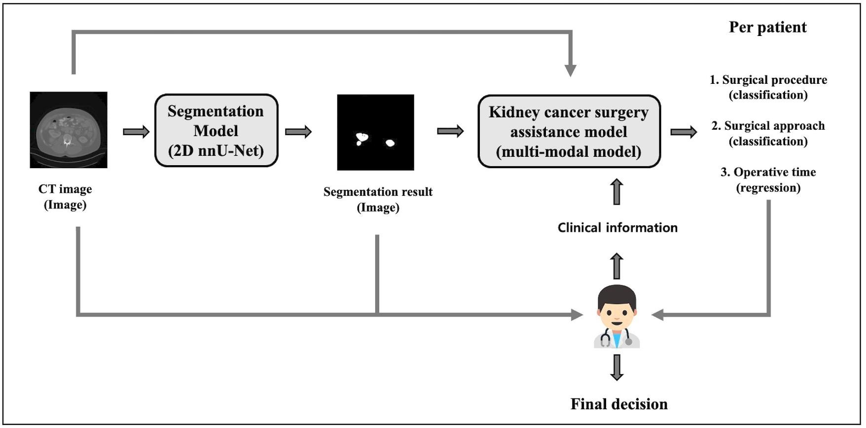
In this study, I propose a two-stage deep learning framework for personalized kidney cancer surgery planning. The first stage performs kidney tumor segmentation from CT images using a 2D nnU-Net model. In the second stage, a multi-modal surgical assistance model takes the largest tumor slice from the segmented CT volume along with clinical features such as radiological tumor size, age, and BMI to recommend the surgical procedure and approach, and predict operative time. By integrating imaging and clinical data, my framework delivers actionable, patient-specific recommendations that support clinical decision-making and enhance operative efficiency.

Methodology

Dataset

Variable	Category / Statistic	Frequency (percentage) / Value
Surgical Procedure	Partial Nephrectomy	138 (66.6%)
	Radical Nephrectomy	69 (33.3%)
Surgical Approach	Transperitoneal	169 (81.6%)
	Retroperitoneal	38 (18.3%)
Operation Time (min)	Maximum	613
	Minimum	44
	Mean	242.29
	Standard Deviation	98.86

Table 1 | Summary of surgical characteristics in the dataset, including the distribution of surgical procedures and approaches, as well as statistics for operation time.

This study utilizes the publicly available C4KC-KiTS dataset, which includes volumetric abdominal CT scans from patients diagnosed with kidney cancer, along with expert-annotated segmentation masks for kidneys and tumors. The dataset is widely used in kidney tumor segmentation research due to its high-quality annotations and comprehensive clinical information. For this study, the dataset was divided into 155 patients for training, $10$ for validation, and $42$ for testing, following standard protocols to ensure robust model evaluation and reproducibility. The data size is 512 by 512 pixels, but since the resolution along the $z$ -axis varies for each patient, the number of slices also differs from patient to patient. To achieve consistent data distribution across slices, I applied min–max normalization individually to each slice of all subjects, scaling pixel intensity values to fall within the range of 0 to 1.

Each patient record contains not only the imaging data but also detailed clinical and procedural metadata. As shown in Table 1, surgical procedures were categorized into partial nephrectomy ( $138$ cases) and radical nephrectomy (69 cases), while surgical approaches were classified as transperitoneal (169 cases) or retroperitoneal (38 cases). Operation times showed wide variability, ranging from 44 to 613 minutes, with a mean duration of approximately 242 minutes and a standard deviation of $98.86$ minutes.

In terms of clinical characteristics, the dataset includes patient age, body mass index (BMI), tumor size, and other relevant variables. Patient ages ranged from 1 to 90 years, with a mean of 58.01 years and a standard deviation of 13.66 years. BMI, calculated as weight in kilograms divided by height in meters squared ( $\mathrm{kg}/\mathrm{m}^2$ ), ranged from $16.2$ to 49.61, with an average of 31.21 and a standard deviation of $6.77$ , indicating a predominance of overweight and obese individuals. Tumor size was quantified by the maximum diameter of the renal mass, ranging from 1.2 cm to 16.2 cm, with an average of $4.6$ cm and a standard deviation of 2.56 cm.

Figure 2 | Architecture of the proposed segmentation model, which follows the standard 2D nnU-Net framework consisting of an encoder–decoder structure with skip connections.

Proposed Deep Learning Framework

The proposed deep learning framework consists of two stages. In the first stage, a $2$ D nnU-Net performs slice-by-slice segmentation. In the second stage, the largest segmented tumor slice per patient, along with clinical information such as age, BMI, and radiological size, is fed into a multi-modal model. This model simultaneously predicts the surgical procedure, surgical approach, and operative time. The framework not only provides kidney tumor segmentation results but also delivers personalized surgical planning recommendations based on both imaging data and patient-specific information.

Segmentation Model

As shown in Figure 2, the segmentation stage is based on a $2$ D nnU-Net architecture, which independently processes each axial CT slice. Segmentation refers to dividing an image into meaningful regions—for example, separating a tumor from surrounding healthy tissue—to enable precise localization and quantification of anatomical structures.

The model consists of an encoder-decoder structure with skip connections, facilitating the preservation of spatial detail while capturing contextual information. An encoder-decoder architecture involves two main parts: the encoder progressively extracts features by reducing spatial dimensions, while the decoder reconstructs the spatial resolution to produce detailed segmentation maps. Skip connections link corresponding layers in the encoder and decoder to preserve fine-grained spatial information that might otherwise be lost during downsampling. From a theoretical perspective, recent advances have provided a unified framework that explains why encoder-decoder CNNs perform effectively. This framework links the architecture to nonlinear frame representations based on combinatorial convolutional frames, with expressivity that grows exponentially as network depth increases. Moreover, skipped connections are shown to significantly enhance the model’s expressive capacity and shape a favorable optimization landscape, helping the network learn robust and coherent geometric features⁹. Each encoder block comprises two convolutional layers followed by batch normalization and leaky ReLU activation, while the decoder mirrors this structure with upsampling layers to reconstruct the segmentation mask.

A convolutional layer, a key part of convolutional neural networks (CNNs) inspired by the animal visual cortex, applies learnable kernels across input images to detect local patterns like edges and textures. These kernels slide over the image’s $2$ D pixel grid, producing feature maps that capture important characteristics and grow more complex through layers. CNNs are trained by optimizing these kernels to minimize errors via backpropagation and gradient descent¹⁰. Batch normalization is a technique that normalizes the output of a layer by adjusting and scaling activations, which helps stabilize and accelerate training by reducing internal covariate shift. Leaky ReLU (Rectified Linear Unit) is an activation function applied after batch normalization; unlike the standard ReLU that zeroes out negative inputs, leaky ReLU allows a small, non-zero gradient for negative values, preventing neurons from becoming inactive and improving model learning¹¹.

The model was trained using variants of the Dice loss function, derived from the Dice similarity coefficient, which measures the overlap between predicted and ground truth masks and is well-suited to handling class imbalance in medical image segmentation. Several hybrid loss functions (Dice + Cross-Entropy and Dice + Focal) were also tested; however, the plain Dice loss achieved the highest segmentation performance and was therefore adopted as the final loss function. Experiments demonstrated that these weighting strategies interact strongly with the choice of initial learning rate, influencing model performance notably. For instance, varying learning rates of 0.001 and 0.01 yielded differences in average Dice scores across weighting types, highlighting the need to optimize both hyperparameters jointly. Training utilized the Adam optimizer, an adaptive algorithm that dynamically adjusts learning rates per parameter, supporting stable and efficient convergence over 100 epochs¹².

Layer Type	Input Features #	Output Features #	Parameters #
Linear	# of clinical metadata	256	512
ReLU	–	–	–
Linear	256	512	131,584
ReLU	–	–	–
Linear	512	1024	525,312
ReLU	–	–	–
Linear	1024	1024	1,049,600
ReLU	–	–	–
Linear	1024	1024	1,049,600
ReLU	–	–	–

Table 2 | Architecture of the multi-layer perceptron (MLP) in MPL_1. The number of clinical metadata features is variable; the current table assumes a single clinical metadata feature. The total number of trainable parameters in this architecture is approximately 2.76 million.

Layer Type	Input Features #	Output Features #	Parameters #
Linear	3072	4096	12,587,008
ReLU	–	–	–
Dropout	–	–	–
Linear	4096	2048	8,390,656
ReLU	–	–	–
Dropout	–	–	–
Linear	2048	1024	2,098,176
ReLU	–	–	–
Dropout	–	–	–
Linear	1024	512	524,800
ReLU	–	–	–
Dropout	–	–	–

Table 3 | Architecture of the MPL_2. The input consists of 3072-dimensional features obtained by concatenating 2048-dimensional features from ResNet50 and 1024-dimensional features from MLP_1. The total number of trainable parameters in this architecture is approximately 23.6 million.

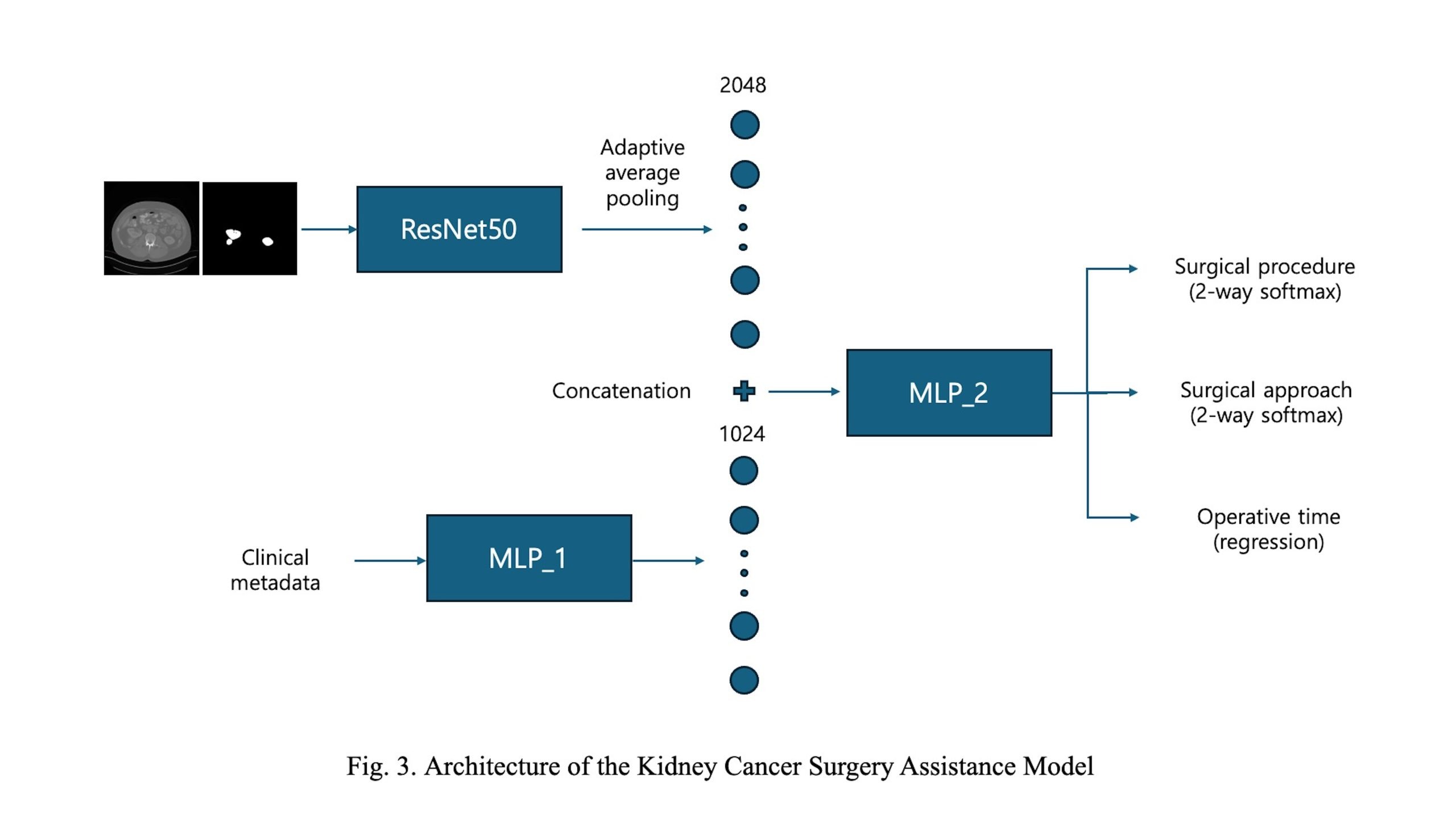
The second stage, referred to as the Kidney Cancer Surgery Assistance Model, is designed to recommend personalized surgical strategies and predict operative time. As illustrated in Figure 3, the model adopts a multi-modal architecture with two distinct branches.

In the first branch, a single axial CT slice containing the largest segmented tumor area—obtained from the segmentation model in the first stage—is used as input. Both the CT image and its corresponding segmentation map are processed by a modified ResNet-50 backbone. The final average pooling and fully connected layers are removed, retaining only the convolutional feature extractor. An adaptive average pooling layer is then applied to the final feature map to produce a fixed-size 2048-dimensional features.
The second branch incorporates patient-level clinical metadata, including radiological tumor size, age, and body mass index (BMI). These numerical features are processed by a multi-layer perceptron (MLP) consisting of five fully connected layers with ReLU activations, resulting in a 1024-dimensional feature embedding. This component is denoted as MLP_1 in Figure 3, and its detailed architecture is provided in Table 2.

The image and clinical feature vectors are concatenated and passed through a shared MLP (MLP_2), which consists of four fully connected layers with dropout regularization. This module produces 512-dimensional latent features. The structure of MLP_2 is detailed in Table~3. From this shared feature, the model branches into three task-specific heads. Two classification heads predict the surgical procedure (2 classes) and surgical approach (2 classes), while a regression head estimates the operative time as a continuous value. This multi-task learning framework enables the model to leverage shared features across tasks, improving learning efficiency while capturing task-specific patterns effectively.
The total loss function for multi-task learning was defined as a weighted sum of task-specific losses, combining binary cross-entropy losses for the classification heads and mean squared error for the regression head, as follows:

(1) $\begin{equation*}L_{\text{total}} = \lambda_{1} L_{\text{procedure}} + \lambda_{2} L_{\text{approach}} + \lambda_{3} L_{\text{operative time}}\end{equation*}$

Where $\lambda_{1} = 1$ , $\lambda_{2} = 1$ , and $\lambda_{3} = 0.00001$ , $L_{\text{procedure}}$ and $L_{\text{approach}}$ denote binary cross-entropy losses for classification tasks, while $L_{\text{operative time}}$ represents the mean squared error loss used for the regression task.

Results

Performance Metrics

The performance of the segmentation model was evaluated using the Dice similarity coefficient (DSC), which quantifies the overlap between predicted and ground truth masks. For the Kidney Cancer Surgery Assistance Model, classification accuracy and mean absolute error (MAE) were used¹³^‘¹⁴.

DSC

The Dice Similarity Coefficient (DSC) is a widely used metric to evaluate the accuracy of image segmentation by quantifying the spatial overlap between the predicted segmentation mask and the ground truth mask. Mathematically, it is defined as:

(2) $\begin{equation*}\text{DSC} = \frac{2 \left| A \cap B \right|}{\left| A \right| + \left| B \right|}\end{equation*}$

where $A$ represents the set of pixels in the predicted segmentation and $B$ represents the set of pixels in the ground truth. The numerator $2 \left| A \cap B \right|$ corresponds to twice the number of pixels common to both sets, while the denominator sums the total pixels in both sets. The DSC ranges from 0 to 1, where 1 indicates perfect overlap and 0 indicates no overlap at all. This metric balances sensitivity to false positives and false negatives, making it particularly suitable for medical image segmentation tasks where precise segmentation of anatomical structures is critical. The DSC has been extensively validated in clinical applications such as brain and prostate tumor segmentation, demonstrating its robustness as a spatial overlap index. It is important to note that while DSC provides a clear measure of segmentation overlap, it may be biased by the size of the target region, with smaller structures often resulting in lower DSC values despite accurate segmentation.

MAE

The Mean Absolute Error (MAE) is used to evaluate the accuracy of regression models, such as the prediction of operative time in surgical assistance systems. It is defined as:

(3) $\begin{equation*} \text{MAE} = \frac{1}{n} \sum_{i=1}^{n} \left| y_i - \widehat{y}_i \right| \end{equation*}$

where $y_i$ is the true value, $\widehat{y}_i$ is the predicted value, and $n$ is the total number of samples. MAE represents the average absolute difference between predicted and actual values, providing an intuitive measure of prediction error magnitude without regard to direction. Unlike metrics that square errors, MAE treats all deviations linearly, making it less sensitive to outliers but still effective in quantifying average prediction accuracy. In clinical contexts, MAE offers a straightforward interpretation of how close predicted operative times are to actual durations, which is critical for surgical planning and resource allocation.

Model stage performance

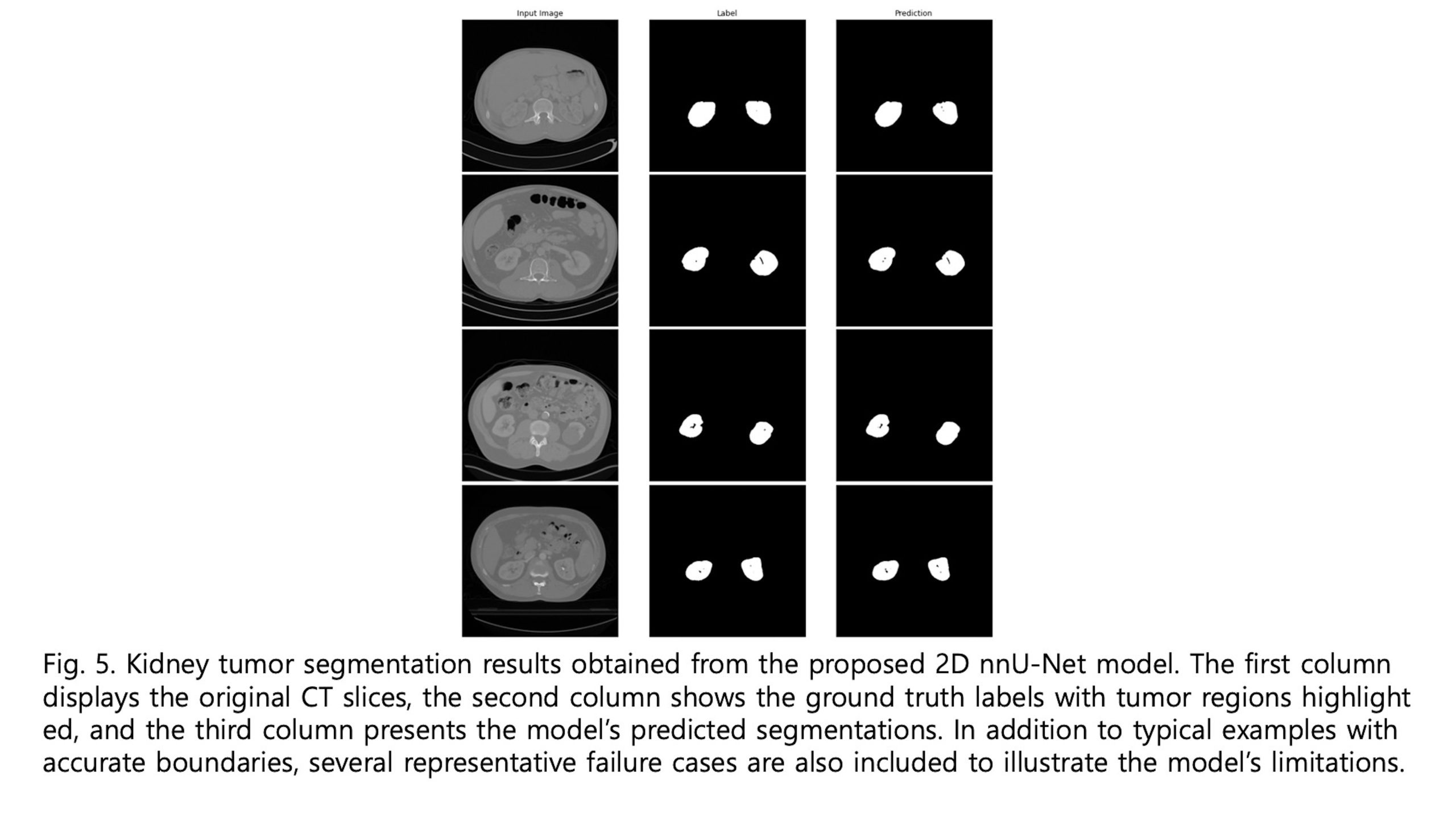
The segmentation model architecture achieved high accuracy in segmenting kidney tumors from CT images, with a Dice score of $0.9247 \pm 0.093$ ( $95%$ CI: $0.881$ — $0.968$ ). In contrast, a conventional U-Net trained under the same settings achieved a lower Dice score of $0.887 \pm 0.102$ ( $95%$ CI: $0.842$ — $0.931$ ). As illustrated in Figure 4, the boxplot and violin plot provide a clear depiction of the distribution of Dice scores across patients, highlighting both the overall consistency and variability of the segmentation performance. As shown in Figure 5, visual inspection of the segmentation results reveals that while minor discrepancies are observed within the internal regions of the tumor, the model accurately captures the overall tumor boundaries. This suggests that the segmentation model effectively learns the global structure of the tumor, even if slight variations exist in pixel-level predictions.

Method	Surgical procedure accuracy (95% CI)	Surgical approach accuracy (95% CI)	Operative time MAE (95% CI, min)
Only image input	76.3% (69.5%, 82.9%)	83.1% (77.1%, 88.3%)	76.4 (67.9, 85.2)
Image + Age	75.9% (69.0%, 82.3%)	81.0% (74.3%, 86.9%)	77.1 (68.2, 86.7)
Image + BMI	78.6% (72.3%, 84.5%)	81.4% (75.0%, 86.8%)	73.5 (65.4, 81.8)
Image + radiological size	85.4% (80.2%, 90.1%)	81.0% (75.1%, 86.2%)	70.8 (63.1, 78.2)
Image + BMI + radiological size	84.9% (79.6%, 89.5%)	78.8% (72.4%, 84.6%)	73.7 (65.5, 82.1)

Table 4 | Quantitative performance results of the Kidney Cancer Surgery Assistance Model across classification and regression tasks.

Method	Confusion matrix	Class	Precision	Recall	F1-score
Surgical Procedure	Actual partial (138) 123 (TP) 15 (FN)	Partial Nephrectomy	0.90	0.89	0.89
Surgical Procedure	Actual radical (69) 13 (FP), 56 (TN)	Radical Nephrectomy	0.79	0.81	0.80
Surgical Approach	Actual transperitoneal (169) 150 (TP), 19 (FN)	Transperitoneal	0.95	0.89	0.92
Surgical Approach	Actual Retroperitoneal (38) 8 (FP), 30 (TN)	Retroperitoneal	0.61	0.79	0.69

Table 5. Confusion matrices and per-class performance for surgical procedure and surgical approach classification using the Image + Radiological Size inputs. The table presents true positives (TP), false negatives (FN), false positives (FP), and true negatives (TN) for each class, along with the corresponding precision, recall, and F1-scores.

Table 4 and Table 5 present results for the multi-modal surgical assistance model evaluated under different input feature combinations. When only imaging features were used, the model achieved 76.3% accuracy in predicting the surgical procedure and 83.1% accuracy for surgical approach classification, with an MAE of 76.4 minutes for operative time prediction. Incorporating patient age alongside imaging features did not improve surgical procedure accuracy and slightly reduced surgical approach accuracy to 81.0%, with a marginal increase in MAE to 77.1 minutes. Adding BMI to imaging inputs improved surgical procedure accuracy to 78.6% and reduced MAE to 73.5 minutes, indicating that patient body composition contributes meaningfully to operative time estimation and procedure selection. The most significant improvement in surgical procedure prediction was observed when radiological tumor size was included with imaging data, raising accuracy to 85.4% and lowering MAE to 70.8 minutes. This highlights the critical role of tumor size in determining surgical strategy and operative complexity. Interestingly, surgical approach accuracy remained relatively stable around 81.0% with the addition of tumor size, suggesting that imaging features alone may be sufficient for this classification task. Combining BMI and tumor size with imaging maintained the highest procedure accuracy (84.9%) but slightly decreased surgical approach accuracy to 78.8% and increased MAE to 73.7 minutes, possibly due to feature redundancy or interactions. The surgical approach appears to depend mainly on anatomical features evident in CT images rather than on clinical characteristics.

Discussion

I developed a segmentation model based on the 2D nnU-Net architecture. While the 3D nnU-Net generally offers superior performance, it also has significant drawbacks, including higher GPU memory consumption and longer inference time. In my study, however, I was unable to utilize the 3D nnU-Net due to the inconsistency in the z-axis resolution and the anatomical coverage of CT scans across patients. If only one of these factors had varied—for instance, if only the z-axis resolution differed—interpolation could have addressed the issue. Alternatively, if only the scanned anatomical range varied, I could have manually cropped the kidney region. However, due to the simultaneous variation in both aspects, applying a 3D model was not feasible. Moreover, the large disparity in z-axis resolution was expected to significantly degrade the performance of a 3D model, justifying my use of the 2D nnU-Net.

The second-stage model, the Kidney Cancer Surgery Assistance Model, faced similar constraints. Ideally, a 3D volume input per patient would allow for more comprehensive predictions of surgical procedure, surgical approach, and operative time. However, due to the aforementioned limitations, I adopted a strategy of selecting a single axial slice with the largest estimated tumor region. I then input both the CT image and its corresponding segmentation mask for that slice to maximize model performance. As shown in Table 4 and Table 5, this approach yielded promising results.

To further enhance performance, I conducted an ablation study with available clinical metadata. Interestingly, some metadata improved model performance when included, while others led to performance degradation. As shown in Figure 6, radiological size emerged as a statistically significant clinical feature correlated with improved performance in the second-stage model. These findings are consistent with the results reported in Table 4 and Table 5. Radiological size was associated with surgical procedure selection and showed moderate correlation with operative time. Given that operative time can vary significantly depending on the individual surgeon, and dataset includes surgeries performed by multiple surgeons across training and test sets, a degree of prediction error is expected. I hypothesize that incorporating surgeon-specific data—such as surgical experience—could further improve model accuracy for operative time prediction.

Although the current mean absolute error exceeds one hour, this level of deviation may still offer practical insight for preoperative planning, particularly in estimating relative surgical complexity and resource requirements across diverse cases. Future work will aim to reduce this error by integrating surgeon-specific and intraoperative variables.

Conclusion

This study presents a practical and effective two-stage deep learning framework for personalized kidney cancer surgery planning. By leveraging a 2D nnU-Net model, I achieved high-accuracy kidney tumor segmentation despite challenges posed by variable CT scan resolutions and anatomical coverage that limited the use of 3D models. My multi-modal surgical assistance model, integrating imaging data with selected clinical features such as radiological tumor size and BMI, demonstrated notable improvements in predicting surgical procedures and operative time. Statistical analysis highlighted radiological tumor size as a key factor correlated with enhanced model performance, underscoring its clinical importance in surgical decision-making. While the adoption of a single axial slice with the largest tumor area provided promising results, incorporating full 3D volume data and surgeon-specific factors such as experience may further enhance predictive accuracy, particularly for operative time estimation. Additionally, the relatively limited dataset size and the absence of external validation cohorts should be acknowledged as constraints that may affect generalizability. Future work should therefore explore these directions alongside larger and more diverse datasets to comprehensively validate and extend the applicability of the proposed framework.

Moreover, future extensions could leverage federated learning frameworks to enable cross-institutional validation without data sharing, or apply transfer learning strategies to adapt the model to institution-specific imaging distributions and surgical practices. These approaches would help generalize the framework across diverse clinical settings while preserving patient data privacy.

References

M. P. Hoenig and G. A. Hladik, “Overview of kidney structure and function,” in National Kidney Foundation’s Primer on Kidney Diseases: Elsevier, (2018), pp. 2-18. [↩]
N. J. Vogelzang and W. M. Stadler, “Kidney cancer,” The Lancet, vol. 352, no. 9141, pp. 1691-1696, (1998). [↩]
I. Sluimer, M. Prokop, and B. Van Ginneken, “Toward automated segmentation of the pathological lung in CT,” IEEE transactions on medical imaging, vol. 24, no. 8, pp. 1025-1038, (2005). [↩]
S. Bachanek et al., “Renal tumor segmentation, visualization, and segmentation confidence using ensembles of neural networks in patients undergoing surgical resection,” European Radiology, vol. 35, no. 4, pp. 2147-2156, (2025). [↩]
W. Zhao, D. Jiang, J. P. Queralta, and T. Westerlund, “Multi-scale supervised 3D U-Net for kidneys and kidney tumor segmentation,” arXiv preprint arXiv:2004.08108, (2020). [↩]
S. Mahmud, T. O. Abbas, A. Mushtak, J. Prithula, and M. E. Chowdhury, “Kidney cancer diagnosis and surgery selection by machine learning from CT scans combined with clinical metadata,” Cancers, vol. 15, no. 12, p. 3189, (2023). [↩]
M. Mahootiha, H. A. Qadir, J. Bergsland, and I. Balasingham, “Multimodal deep learning for personalized renal cell carcinoma prognosis: integrating CT imaging and clinical data,” Computer Methods and Programs in Biomedicine, vol. 244, p. 107978, (2024). [↩]
K. Sun et al., “Medical multimodal foundation models in clinical diagnosis and treatment: Applications, challenges, and future directions,” arXiv preprint arXiv:2412.02621, (2024). [↩]
J. C. Ye and W. K. Sung, “Understanding geometry of encoder-decoder CNNs,” in International Conference on Machine Learning, (2019): PMLR, pp. 7064-7073. [↩]
R. Yamashita, M. Nishio, R. K. G. Do, and K. Togashi, “Convolutional neural networks: an overview and application in radiology,” Insights into imaging, vol. 9, no. 4, pp. 611-629, (2018). [↩]
Y. Chen, X. Dai, M. Liu, D. Chen, L. Yuan, and Z. Liu, “Dynamic relu,” in European conference on computer vision, (2020): Springer, pp. 351-367. [↩]
C. Shen et al., “On the influence of Dice loss function in multi-class organ segmentation of abdominal CT using 3D fully convolutional networks,” arXiv preprint arXiv:1801.05912, (2018). [↩]
M. Hutton, E. Spezi, C. Doherty, A. Duman, and R. Chuter, “Investigating the feasibility of MRI auto-segmentation for Image Guided Brachytherapy,” in Engineering Research Conference (2023), p. 11. [↩]
C. J. Willmott and K. Matsuura, “Advantages of the mean absolute error (MAE) over the root mean square error (RMSE) in assessing average model performance,” Climate research, vol. 30, no. 1, pp. 79-82, (2005). [↩]

Deep Learning Framework for Kidney Tumor Segmentation with Surgical Method Recommendation and Operative Time Prediction

Abstract