AMS-Aware Deep Learning for Higgs Boson Classification

Abstract

In high-energy physics(HEP), identifying rare signal events such as Higgs boson decays in background noise is a central challenge. Traditional machine learning approaches rely on standard loss functions like binary cross-entropy(BCE), which are not directly aligned with domain-specific evaluation metrics. In this work, I revisit the Higgs Boson Machine Learning Challenge datasets and propose a deep neural network classifier trained using an approximate median significance (AMS)-aware loss function¹. This loss optimizes for the significance used in particle physics, allowing the model to prioritize high-confidence signal identification. I compare the AMS-optimized deep learning model against a baseline neural network trained with standard cross-entropy. For evaluating each model, I submitted a prediction file from each and compared their AMS scores from Kaggle. Furthermore, I used bootstrapping to run significance tests on the difference in their scores. Experimental results show that the BCE-loss model achieved an AMS score of 2.78876 while the AMS-loss model achieved a score of 2.96330. Also, during bootstrapping with 1000 iterations, the AMS-loss model outperformed the BCE-loss model in every one. When calculating the area under the receiver operating characteristic curve (AUC-ROC or AUC) score of each model, the BCE-loss model had a score of 0.928 and the AMS-loss model had a score of 0.905. Although the BCE-loss model outperforms the AMS-loss model, a score above 0.9 is still considered great discrimination. AMS-aware training achieves higher AMS while maintaining competitive AUC, which is better suited for experimental research in particle physics.

1. Introduction 

The discovery of the Higgs Boson at the Large Hadron Collider (LHC) marked a major milestone in particle physics, confirming the mechanism that gives mass to elementary particles. Yet, even after this breakthrough, continued analysis of proton-proton collisions is essential for characterizing Higgs properties and searching for new physics beyond the Standard Model. A central challenge in this effort lies in distinguishing rare signal events from the overwhelmingly large background generated by known processes.

Machine learning (ML) methods have become essential tools in high-energy physics (HEP) for tasks such as event classification, particle identification, and anomaly detection^2,3. In particular, the 2014 Higgs Boson Machine Learning Challenge provided a benchmark dataset of simulated collision events to evaluate classification models on the task of identifying Higgs-like signals¹. In their seminal work, Baldi et al. demonstrated that deep neural networks (DNNs) could outperform traditional models by learning from high-level engineered features, helping bridge the gap between physics-driven and data-driven approaches⁴.

Despite these advances, a common limitation persists: most models are trained using generic loss functions such as binary cross-entropy (BCE), which are agnostic to the physics-driven goals of the task. In contrast, the standard evaluation metric in HEP for signal discovery is the Approximate Median Significance (AMS) — a nonlinear function that accounts for both the number of correctly identified signal events and the background contamination. Training with BCE may lead to models that perform well in terms of accuracy or AUC-ROC, but not necessarily in terms of AMS, which is the main criterion for scientific discovery in physics.

In this paper, I propose a deep learning classifier trained with an AMS-aware loss function, designed to directly optimize for the discovery significance used in experimental HEP. I implement a differentiable approximation of the AMS metric and use it to guide model updates during training. I compare this approach to a baseline model trained with BCE loss, evaluating model performance in terms of AUC and AMS. No CNNs (convolution neural networks) were considered, since they don’t do well with noisy data.

The results show that AMS-aware training improves discovery sensitivity, producing classifiers that better align with the physics objectives of the Higgs classification task. This work highlights the potential of physics-informed machine learning to enhance signal detection and improve the interpretability and relevance of ML models in scientific applications.

2. Methodology

For training, I use the dataset provided by the Higgs Boson Machine Learning Challenge hosted by Kaggle in collaboration with CERN and ATLAS. The dataset has simulated proton-proton collision events, under both signal and background hypotheses, with event-level features to facilitate classification¹.

The dataset is composed of three CSV files:

train.csv: 250,000 labeled events, each with an associated weight and a label (‘s’ for signal, ‘b’ for background).
test.csv: 550,000 unlabeled events, used in the original challenge for private evaluation.
random_submission.csv: An example Kaggle submission to provide formatting guidelines.

Although the datasets are imbalanced, no dataset balancing techniques were considered since the data was already representative of real-world experiment data. To maintain this representation, no techniques were used. Furthermore, the Kaggle dataset was created using the official ATLAS full detector simulator, which means it is fully representative of real-life data.

Each event includes 30 high-level features, derived from reconstructed physics objects such as jets, leptons, and missing transverse energy. These features are grouped into:

DER (derived features): calculated using domain knowledge.
PRI (primary features): raw measurements from detectors.

Additionally, each event includes a weight representing event importance, based on its frequency in simulation; A unique identifier called event ID; and a label: ‘s’ (signal) or ‘b’ (background).

I applied several preprocessing steps before training. Some features include a placeholder value of -999.0 to indicate missing or undefined measurements. These were replaced with NaN, and then imputed using the mean of the feature across the dataset. The ‘Label’ column was mapped to binary format: ‘s’ → 1, ‘b’ → 0.

After these preprocessing steps, I started the initial training of the model along with hyperparameter tuning:

The train.csv data was split using Scikit-learn’s stratified k-fold cross validation function with 3 folds.

All numerical features were standardized using the StandardScaler feature from the Scikit-learn library to ensure zero-mean and unit-variance, which improves convergence during neural network training.

For the BCE loss function, I used PyTorch’s nn.BCE feature which allows easy use of the BCE metric for neural network training. The BCE loss calculation is as follows:

   

where is the true label and is the predicted probability.

For the AMS loss function, I used a differentiable approximation of the actual metric since the actual metric is non-differentiable and therefore can’t be used as a loss function. The actual metric is defined as:

   

where is the sum of weights for true positive signal predictions, is the sum of weights for false positive background predictions, and is a small regularization term (set to ).

The regularization term is added so that if the sum of weights for false positive background predictions is , the function doesn’t become undefined.

Since this is non-differentiable, I implemented a differentiable approximation that estimates and using the predicted probabilities:

   

I define the AMS-aware loss as the negative of the AMS score:

   

This is done to make the minimization of the AMS loss a maximization of the AMS metric.

The accuracy of this approximation is proven by the stability of the model during training and also the reduced AMS loss. This proves that the approximation effectively increases the AMS metric, since it is representative of the actual function.

After defining these functions, I converted the data to PyTorch tensors (float32) to be used in neural network training⁵. I also put sample weights into the loss function during training for the AMS-loss function since it required those. These weights weren’t added for the BCE-loss model’s training since it wasn’t required for calculation.

During this initial training, I used the Optuna library to optimize hyperparameters for each model. Using the suggest_ functions, I was able to give values to be tested within the trials. I ran Optuna with 50 trials.

After finding the best hyperparameter values, I evaluated 2 deep learning neural networks for the task of Higgs boson signal classification and expanding on Baldi et. al’s work:

First, the BCE-loss model, which contained 5 hidden neuron layers with 384 neuron units each, using ReLU activation. This model used a dropout rate of around 0.256 for overfitting prevention, and a learning rate of approximately 0.000267. The batch size for weight updates during training was 64 values.

Second, the AMS-loss model ,which contained 2 hidden neuron layers with 448 neuron units each, also using ReLU activation. This model used a dropout rate of around 0.187 for overfitting prevention, and a learning rate of approximately 0.00108. The batch size for weight updates during training was 256 values.

Both models used the Adam optimizer from PyTorch with the learning rates from Optuna.

The models were evaluated mainly on 2 metrics: AUC-ROC and AMS. 

The AUC-ROC metric is used commonly within standard binary classification tasks for machine learning, and it penalizes models for incorrect classifications with high confidence. Essentially, it rewards high confidence for accurate classifications.

The AMS metric is used commonly within HEP model evaluation for binary classification tasks. It measures the likelihood of observed events being signal events rather than random fluctuations in background noise. This metric fits HEP classification tasks, since background noise fluctuates significantly. For model evaluation, it measures how well it can separate these fluctuations from actual signals.

First, I used a training iteration with 3 folds on the train.csv dataset to compare the average AUC-ROC and AMS scores of the BCE-loss and AMS-loss models. During this, I also graphed the training loss vs. time(epochs) and validation AMS vs. time(epochs) to check for overfitting and confirm an optimal number of epochs to train each model for.

Second, I created submission prediction datasets for both models on the test.csv dataset and submitted them to Kaggle to compare their AMS score performance.

For significance testing, I used bootstrapping with 1000 iterations across a set of predictions that each model made on 3 folds of the train.csv dataset. The conditions for significance testing with bootstrapping were checked. 2 significance tests were run to evaluate difference in AMS scoring and AUC-ROC scoring.

After all analyses were done, I created different graphs to visualize the differences in the AMS-loss model and the BCE-loss model.

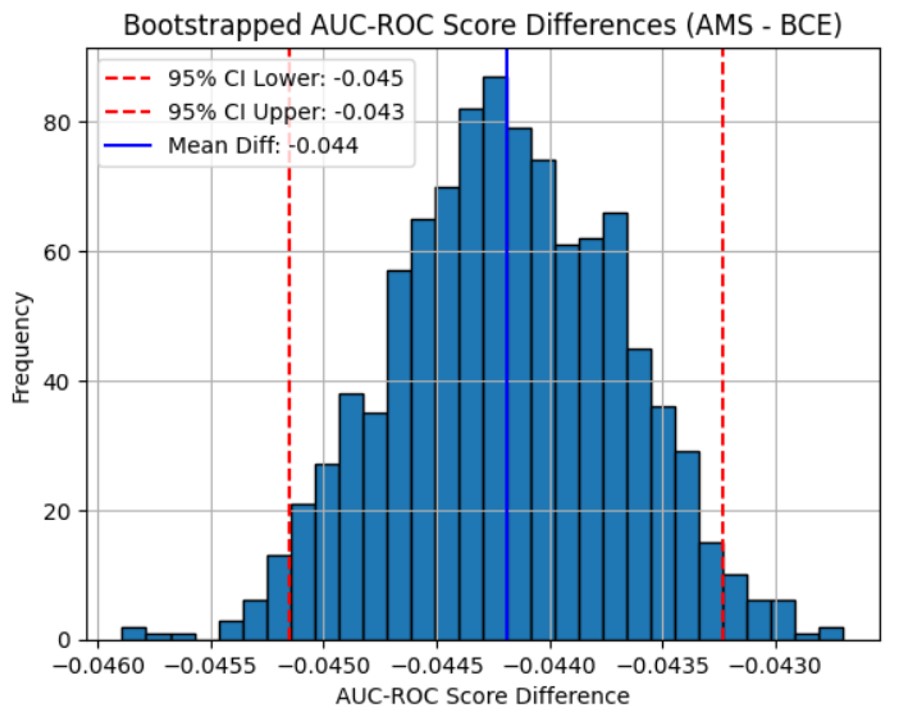
First, I graphed the bootstrapped differences in AMS and AUC-ROC from the AMS-loss model and the BCE-loss model to visualize the confidence interval that was created for the differences in each score.

Second, I graphed the ROC curves for each model to evaluate their AUC-ROC scores during the bootstrapping test.

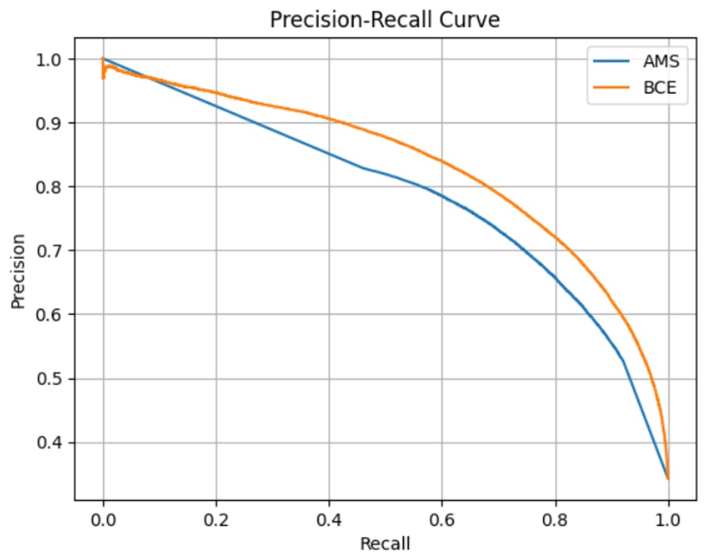
For the last two graphs, I plotted the precision-recall curve and the cumulative AMS curve for each model to visualize their effectiveness in handling imbalanced data and large amounts of background noise, which are two commonly occurring problems in standard tasks and physics objectives, respectively.

3. Results

In their work, Baldi et al. utilized a simulated dataset similar to the Kaggle datasets. Their main metric for evaluation was AUC-ROC.

Kaggle’s Higgs Boson Machine Learning Challenge comes with two datasets: train.csv and test.csv. It also comes with random_submission.csv which provides the format for submission to Kaggle and AMS score computation.

The first step taken was to pre-process the train.csv and test.csv datasets. Missing values were noted with the value -999.0, and these were replaced with mean imputation. The first column had the EventId label, which was dropped since it provided no use for training.

After pre-processing, initial training was done alongside hyperparameter tuning. Both neural network models were implemented in PyTorch and Scikit-learn and trained on a system with CPU only. The first step taken was hyperparameter tuning for each model. During tuning, the training set was split using stratified k-fold cross validation with 3 folds for each iteration. Each iteration was done with 10 epochs. Dataset folding was done using Scikit-learn and hyperparameter optimization was done using the Optuna library, which provides easy tuning with suggested parameter values. For the BCE-loss model, the parameters suggested were the number of hidden layers, the size of each hidden layer, the dropout rate, the learning rate, and the batch size for a full pass. After tuning, these were the optimized parameters for the BCE-loss model:

n_layers = 5
hidden_size = 384
dropout = 0.2563994979733446
lr = 0.00026724473332425096
batch_size = 64

For the AMS-loss model, the hyperparameters being tuned were the same as the previous model. After tuning, these were the optimized parameters for the AMS-loss model:

n_layers = 2
hidden_size = 448
dropout = 0.18657792297018724
lr = 0.0010795586890825545
batch_size = 256

For both models, suggested values and step counts were the same.

Hyperparameter	Suggested Value
Number of layers	2, 5
Hidden layer size	64, 512, step = 64
Dropout rate	Between 0.1, 0.5
Learning rate	1e-4 to 1e-2
Batch size	64, 128, 256

After tuning, final training and evaluation was done using the optimized hyperparameter values. 3 models were trained for each loss function using the Scikit-learn stratified k-fold cross validation function with k=3. For each model, the average scores were computed for AUC-ROC, Accuracy, and AMS. During this, training loss vs. time (epochs) and validation AMS vs. time (epochs) were also graphed to check for overfitting.

The results for average scores were as follows for the BCE-loss and AMS-loss models:

	AMS-loss	BCE-loss
AUC-ROC	0.8567	0.8992
Accuracy	0.8026	0.8296
AMS	1.6312	1.5865

The training loss vs. time (epochs) and validation AMS vs. time (epochs) graphs are as follows:

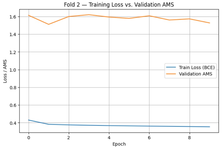
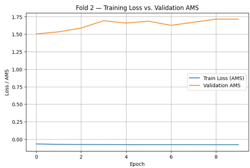
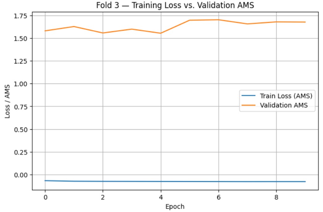
After determining the optimal number of epochs as 10, one final model was trained for both the BCE-loss and AMS-loss using the entire train.csv dataset, with optimized hyperparameters and training time. After generating predictions for each model, they were exported as CSV files and submitted to Kaggle for evaluation. After submission, the AMS scores for both models were as follows:

	AMS Score from Kaggle
AMS-loss	2.96330
BCE-loss	2.78876

After evaluating through Kaggle, further significance testing was done using confidence intervals and bootstrapping. This was done using predictions from 3 folds of the train.csv dataset for each model. For bootstrapping, the results were as follows.

The null hypothesis for AMS significance testing is that the average AMS score of the AMS-loss model is the same as the average AMS score of the standard BCE-loss model. The alternative: The average AMS score of the AMS-loss model is higher than the average AMS score of the standard BCE-loss model. This test meets the following core conditions of bootstrapping for significance testing:

• Observation Independence: each row in the dataset train.csv is independent of each other, and the models during training make each prediction independently of any other predictions it has made. This condition is met.
• Representative Sample: the training.csv dataset is representative of the population (real particle collision events), as it was modeled on the real ATLAS experiments at CERN. This condition is met.
• Sufficient Sample Size: the sample size for this is easily larger than 30, given the original training.csv dataset contains 250,000 events. This condition is met.

With 1000 iterations, the mean difference in AMS scores (AMS model – BCE model) was around 0.1173. The 95% confidence interval for the difference in AMS score between the AMS-loss model and the standard BCE-loss model was the range from 0.0891 to 0.1447. The p-value for the bootstrapping analysis on AMS score is exactly 0. Therefore, the null hypothesis is rejected since the p-value is below any reasonable significance level.

The null hypothesis for AUC-ROC is that the average AUC-ROC score of the AMS-loss model is the same as the average AUC-ROC score of the standard BCE-loss model. The alternative: the average AUC-ROC score of the AMS-loss model is lower than the average AUC-ROC score of the standard BCE-loss model. This test meets the core conditions of bootstrapping for significance tests as described in the previous section.

With 1000 iterations, the mean difference in AUC-ROC scores (AMS model – BCE model) was around -0.0442. The 95% confidence interval for the difference in AUC-ROC score between the AMS-loss model and the standard BCE-loss model was the range from -0.0452 to -0.0432. The p-value for the bootstrapping analysis is exactly 1.

For visualization, the following graphs were created:

4. Discussion

The results show that training with an AMS-aware loss function can improve classification tasks in HEP, like Higgs boson identification. Traditional methods of BCE loss optimize general classification performance, but do not improve AMS, the metric used to reflect discovery sensitivity in particle physics experiments.

When analyzing the Kaggle competition’s AMS evaluation, we can see that on the same dataset, the AMS-loss model was able to achieve a much higher score of 2.96330 compared to the BCE-loss model’s 2.78876.

Furthermore, when analyzing the bootstrapping significance test results, we can see that the AMS-loss model consistently achieves higher AMS scores than the BCE-loss model, as out of 1000 iterations, the AMS-loss model outperforms the BCE-loss in every single one.

However, while the AMS-loss model achieves higher scores in the AMS metric consistently, the BCE-loss model outperforms the AMS model in the AUC-ROC metric in the same way. Similar to the bootstrapping significance test for AMS, the BCE-loss model outperformed the AMS-loss model in every single iteration out of 1000.

One metric where the AMS-loss model doesn’t perform nearly as well as the BCE-loss model is in their precision-recall curves as seen in Figure 12. The curve for the BCE-loss model bends much more to the top-right of the graph, indicating that the BCE-loss model does much better with imbalanced data.

Furthermore, AMS can be an unstable metric with smaller amounts of data, leading to large instability when training with a fold number higher than 4 or 5.

As for the viability of the AMS-loss model, although it underperformed the BCE-loss model in AUC-ROC, it still managed to achieve a score of 0.905 as seen in Figure 11. In general, an AUC-ROC score of over 0.9 is considered great discrimination between signal and background, so the AMS-loss model is still a great classifier when considered in standard classification tasks. Furthermore, the AMS-loss model has a much more stable cumulative AMS curve than the BCE-loss model as seen in Figure 13, which indicates that it would have better classification over large amounts of background data compared to the BCE-loss model. As for the instability of the AMS metric with small datasets, this issue is rarely present in physics classification tasks. The amount of data that a cycle of collisions produces is more than enough to prevent instability in the AMS metric – which is why it is used commonly in HEP.

Combining all of these analyses, we can detail what each model is suited for in classification tasks:

The AMS-loss model does much better with separating random fluctuations in background from signal events, as well as maintaining stable predictions with large proportions of background noise to signal events in data. This is much more physics-informed compared to the BCE-loss model, leading to the AMS-loss model outperforming the BCE-loss model when tasked with a physics-oriented classification task like the Kaggle Higgs Boson Machine Learning Challenge.

The BCE-loss model does much better with handling imbalanced datasets and also consistently achieves higher AUC-ROC scores, which indicates high confidence in correct classification. This is much more oriented towards standard binary classification tasks and will outperform the AMS-loss model which expects random fluctuations in background noise that are usually present in physics datasets.

Overall, the analysis of the experiment with AMS-loss showed that an AMS-aware model is much more oriented towards physics classification objectives than the standard BCE-loss model.

5. Conclusion

In HEP, a common struggle with neural network classification is that standard loss functions like BCE-loss fail to separate random fluctuations in background noise from actual signal events due to overconfidence in classifying false positives. To solve this issue, I propose the use of a differentiable approximation of the commonly used AMS metric within neural network loss functions during training to create more physics-informed classification models.

To implement this proposed loss function, I compared its performance in the AMS and AUC-ROC metrics to that of a standard BCE-loss model, using the Kaggle Higgs Boson Machine Learning Challenge dataset to train and evaluate the models.

I found that the AMS-loss model consistently outperformed the BCE-loss model in terms of AMS, but underperformed in the AUC-ROC metric. However, while it underperformed, it still achieved an AUC-ROC score that indicated great discrimination between signal and background, which makes the model feasible for even standard classification tasks. This proves that it can improve physics-specific classification without sacrificing general classification quality. 

Furthermore, the AMS-loss model outperforms the BCE-loss model when faced with higher amounts of highly fluctuating background noise, which is common in HEP.

Comparing this to Baldi et. al’s work, they achieved an AUC-ROC score of 0.88 on a similarly synthesized HIGGS dataset⁴. The AMS-loss I proposed was instead able to achieve a higher score of 0.905. Some reasons for this may be that the HIGGS dataset is more imbalanced than the Kaggle one, or that the model proposed in Baldi et. al’s paper is overfitting to the data. Furthermore, they stated that they could not thoroughly tune hyperparameters due to computational costs, so that may have also been a factor.

Future directions include applying AMS-aware training to real experimental data from CMS(Compact Muon Solenoid) experiments or ATLAS(A Toroidal LHC ApparatuS) experiments, extending the approach to ensemble models or uncertainty-aware frameworks, and integrating interpretability tools such as SHAP(SHapley Additive exPlanations) to better understand feature-level contributions to discovery.

References

1. Kaggle. The Higgs Boson Machine Learning Challenge. (2014). [↩] [↩] [↩]
2. J. Duarte, S. Han, P. Harris, S. Jindariani, E. Kreinar, B. Kreis, J. Ngadiuba, M. Pierini, R. Rivera, N. Tran and Z. Wu. Fast inference of deep neural networks in FPGAs for particle physics. Journal of Instrumentation 13 (2018). [↩]
3. A. Radovic, M. Williams, D. Rousseau, M. Kagan, D. Bonacorsi, A. Himmel, A. Aurisano, K. Terao, T. Wongjirad. Machine learning at the energy and intensity frontiers of particle physics. Nature 560, 41–48 (2018). [↩]
4. P. Baldi, P. Sadowski, and D. Whiteson. Searching for exotic particles in high-energy physics with deep learning. Nature Communications 5 (2014). [↩] [↩]
5. A. Paszke, S. Gross, F. Massa, A. Lerer, J. Bradbury, G. Chanan, T. Killeen, Z. Lin, N. Gimelshein, L. Antiga, A. Desmaison, A. Kopf, E. Yang, Z. DeVito, M. Raison, A. Tejani, S. Chilamkurthy, B. Steiner, L. Fang, J. Bai, S. Chintala. PyTorch: An imperative style, high-performance deep learning library. Adv. Neural Inf. Process. Syst. 32 (2019). [↩]