A Machine Learning Framework for Predicting NFL Injuries Based on Preceding-Play Patterns

Abstract

Injuries are an inevitable part of all professional sports. In football, their consequences can impact not only individual players but also entire teams and seasons. As the physical demands of the NFL continue to grow, so does the need for tools that can anticipate and prevent injuries before they occur. This study explores the use of artificial intelligence (AI) and machine learning (ML) to predict injury risk based on game context, player movement, environmental factors, and play history. Using a variety of modeling approaches and resampling strategies to handle severe class imbalance, we found that analyzing sequences of plays leading up to injuries, rather than the injury plays themselves, produced the strongest results. Our best model achieved a recall of 56% and a precision of 40% in detecting injury risk on synthetic data. While still modest, these findings demonstrate that pre-injury play patterns can provide valuable signals for anticipating injury risk, even in highly imbalanced datasets.

Introduction

While previous research has examined the relationship between injury rates and factors like playing surface or weather, much of it has been retrospective or limited to basic statistical analysis¹. Traditional approaches have relied on biomechanics, player interviews, or post-game video review, aiming to understand why injuries happened rather than predict when they might occur². Statistical models, while useful for identifying long-term trends, struggle with play-to-play variability and rarely offer actionable insights in real time³.

This study aims to go further by using machine learning models to actively predict when injuries might occur, based on patterns hidden within large-scale NFL datasets. Unlike traditional research that focuses on a single hypothesis, this paper takes an exploratory approach, testing multiple strategies and angles to see how injury prediction can best be approached.

Simple physical correlations between players and injuries aren’t reliable enough to predict injuries, as overlapping patterns across multiple plays are often what show what could be an upcoming injury waiting to happen.

The goal of this study is not only to evaluate how well different algorithms perform, but also to better understand how injuries might be foreseen. Specifically, this paper aims to:

• Evaluate how well different machine learning algorithms predict injuries
• Investigate whether early signs of injury risk can be detected in play sequences
• Explore whether overlapping patterns across multiple plays are more predictive than single-event features

Methods

Dataset Used and Preprocessing

This study uses a dataset provided by the NFL’s 1st and Future competition on Kaggle, which includes 3 detailed data .csv files: InjuryRecord.csv, PlayList.csv, and PlayerTrackData.csv. These files contain detailed info about each play that was logged by all 250 players for every game, contextual information about each play, and high-resolution tracking data that captures player positions, their movements, and speeds at 0.1-second intervals for every play. The dataset includes only non-contact lower-limb injuries, which were selected by the NFL as part of the competition focus. These injuries are believed to be influenced by surface conditions and player movement rather than direct collisions⁴.

The dataset used for this project was from the NFL 1st and Future competition, which had detailed histories for 250 players, with dozens of plays in a number of games, the game-time conditions for each game, and movement data for each play. Data was preprocessed to first look at key correlations, as well as engineering key features such as playing surface, player position, game temperature, and type of play. Our models were evaluated using accuracy, precision, recall, and F1-score to compare performances, while more advanced comparisons like our Stratified K-fold verified models weren’t just “memorizing” data, a common theme in our early stages of models (more on that in the overfitting explanation).

Injury prediction is inherently much more difficult than it may seem, as there isn’t necessarily a one-to-one relationship between features and outcomes, making it necessary to explore multiple modeling strategies. It’s an extremely complex challenge that can be approached from multiple angles. So, rather than relying on a single strategy or model, various techniques were utilized to understand which types of patterns and signals may precede injuries. Some approaches involved differentiating injury plays from non-injury plays based on basic features like the surface type of the field and the game-time temperature, while others focused on analyzing sequences of plays leading up to an injury, aiming to uncover any potential warning signs in player behavior or game context that could hint at an upcoming injury.

This multi-faceted approach highlights the importance of combining different perspectives, such as single-play classification, temporal analysis, and contextual factors, to build a more complete and realistic injury prediction framework. This paper contributes to the growing usage of AI in sports science, as it demonstrates how tools can be applied to predict injuries in NFL athletes from game-driven data. Hopefully, AI models can identify patterns or signs from a variety of game-related features to point toward a possible future injury, offering a foundation for proactive injury prevention strategies.

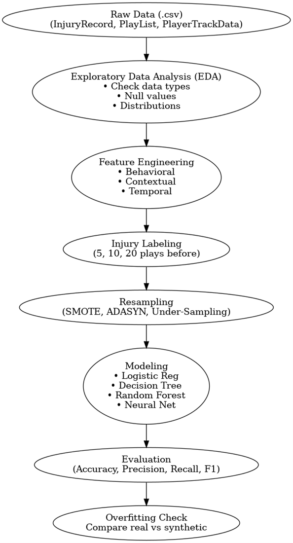
The raw data required extensive cleaning and transformation before modeling, starting with filling in all missing values and removing null values to ensure the models wouldn’t encounter syntax errors or be affected too much by incorrect data. PlayerTrackData.csv included data about the speed, location on the field, and direction for each player frame-by-frame for each 0.1-second interval. We grouped the tracking data by the PlayKey that was associated with each play. The PlayKey included the PlayerKey and GameKey attached to the last number, which indicated the play number (46th play of the game would have a 46). We aggregated the tracking data for each play by computing mean speed (s), total distance traveled (dis), mean direction, standard deviation of direction (dir), and a calculated measure of angular speed based on directional variance across all 0.1-second intervals.
Injured players were identified through InjuryRecord.csv, and their corresponding play keys (PlayKey) were isolated. For modeling, we focused not just on the injury plays themselves but on the preceding plays. Specifically, we explored three window sizes: 5, 10, and 20 plays before an injury. Any play that occurred within N plays before an injury was labeled as a PreInjury = 1, while all others were labeled 0. This approach provided a more proactive and realistic framing for injury prediction.
Because the dataset is limited to non-contact lower-body injuries, which tend to result from accumulated stress or biomechanical factors, it is reasonable to assume that meaningful risk patterns may emerge in the plays leading up to the injury. Labeling these 5–20 plays as “pre-injury” allows for detection of such patterns in advance.
Because of the severe imbalance of injuries to non-injury plays (since injuries are rare compared to all plays), we employed three resampling strategies to balance the data during model training:
SMOTE (Synthetic Minority Oversampling Technique): SMOTE generates synthetic injury samples by interpolating between existing ones. This helps expose the model to more examples of injury plays without simply duplicating the data.

ADASYN (Adaptive Synthetic Sampling): Similar to SMOTE, but it focuses more on difficult-to-learn examples. ADASYN creates more synthetic samples near injury plays that are harder for the model to classify, which can improve performance in tricky edge cases.

Random Under-Sampling: This approach balances the dataset by randomly removing non-injury plays (the majority class). It’s simple and avoids synthetic data, but it can discard potentially useful information.

We chose these techniques because our dataset was highly imbalanced, with far fewer injury plays compared to normal plays. SMOTE and ADASYN allowed us to artificially boost the number of injury examples to give the model more patterns to learn from. Random under-sampling provided a useful contrast, as it uses only real data and avoids overfitting to artificial patterns. Using all three allowed us to test which approach worked best for injury prediction in this imbalanced context⁵.

Exploratory Data Analysis (EDA)

Dataset Overview

To better understand the dataset before modeling, we performed an exploratory data analysis (EDA) on the three core files, focusing on data types, missing values, distributions, and key trends across player behavior and injury patterns.

• InjuryRecord.csv: 105 records of lower-limb injuries, including body part, surface type, and time missed.
• PlayList.csv: 151,987 player-play entries, with info on weather, surface, stadium type, and play type. Most plays are non-injury plays; injury plays can be cross-referenced with InjuryRecord.
• PlayerTrackData.csv: 263,121 plays broken down into 0.1-second intervals, with player location, speed, direction, orientation, and distance moved.

Initial Data Checks

• Missing Values:StadiumType and Weather are missing in 9,484 rows (mostly from indoor stadiums where weather may be irrelevant).
• PlayType is missing in 207 entries.
• Event is missing in most of PlayerTrackData.csv, but this was expected and didn’t affect model development.
• Duplicates:
• No true duplicates, though many rows represent time slices of the same play. This was intentional given the tracking data format.

Visual Analyses

We included several visualizations in the appendix to better understand data patterns.

• Play Type Distribution: Passing and rushing dominate the dataset, while special teams plays are much less common.
• Roster Position Distribution: Most data comes from linebackers, linemen, and wide receivers, as those positions are often involved in high-impact plays.
• Temperature Distribution: Most games occurred between 50–80°F. When split by injury vs. non-injury, no significant difference was visible.
• Correlation Heatmap: Shows low correlation between injury and numeric features. PlayerGame and PlayerDay are highly correlated (r = 0.89), as expected, where r is the Pearson correlation coefficient representing the strength of a linear relationship between two variables.
• Injury by Surface & Body Part: Slightly more ankle injuries on turf; more knee injuries on natural surfaces. This supports existing concerns around synthetic turf and lower-body injuries.

The EDA helped clarify how the data was structured and where its limits were. We saw that injuries were rare and unevenly spread, and most basic stats like temperature or surface didn’t show strong patterns on their own. Some columns had missing values, but nothing that seriously broke the data. These takeaways guided how we cleaned the data, chose features, and set up our injury prediction task.

Feature Engineering

We engineered features across three categories: behavioral/tracking-based, contextual, and temporal. From the player tracking data, we computed metrics such as mean speed, max speed, total distance, and direction changes (mean, standard deviation, and angular speed). Contextual features included environmental and situational data like FieldType, PlayType, Weather, RosterPosition, and StadiumType, all of which were label-encoded after handling missing values. Temporal features included each player’s game number and cumulative plays to reflect progression and fatigue. These engineered features were then used as inputs for model training.
A breakdown of key features across each category:
1. Behavioral/Tracking Features:
Mean Speed / Max Speed: Captures the pace of movement. Faster plays may correlate with higher exertion or risky maneuvers.
Total Distance Traveled: Reflects how much ground the player covered during the play.
Mean Direction / Directional Standard Deviation: Measures how much a player’s movement varied directionally, which might indicate cutting, pivoting, or instability.
Angular Speed: A feature we created to measure how quickly and frequently a player changed direction during a play. It was based on the directional values in the tracking data, which show which way the player was facing or moving every 0.1 seconds. We calculated the variance in direction across each play and used that to estimate how much the player was turning or cutting. The more the direction changed, the higher the angular speed.
2. Contextual Features:
FieldType: Whether the surface was natural grass or synthetic turf. Prior studies suggest turf might raise injury rates.
StadiumType: Indoor vs. outdoor stadiums, which can influence exposure to external conditions.
Weather: General weather conditions (e.g., clear, rainy, snowy) that could impact traction and footing.
Temperature: Numeric value showing game-day temperature, which may affect muscle function or fatigue.
PlayType: Type of play (pass, rush, etc.), giving the model context around player movements.
RosterPosition: Player’s on-field role (WR, RB, OL, etc.), since injury risk varies across positions.
3. Temporal Features:
GameNumber: How many games the player had appeared in so far that season.
CumulativePlays: Total number of plays a player had participated in. While this doesn’t account for rest days, practice loads, or injury history, it served as a proxy for accumulated game fatigue. Ideally, more advanced metrics like acute-to-chronic workload ratios would have been used, but that kind of data wasn’t available. So this feature was a practical stand-in to reflect overall in-game wear and tear.

These features were picked to give some context around fatigue and exposure. They’re not perfect, but they still helped the model get a sense of whether a player had been on the field a lot and might be more at risk.
Categorical features such as FieldType, PlayType, RosterPosition, StadiumType, and Weather were label-encoded numerically using scikit-learn’s LabelEncoder. Numeric features such as Temperature were retained as continuous variables. Any missing values were filled with 0. Encoding was needed for categorical variables since machine learning models work best when they process numerical data⁶.

Injury Labeling and Prediction Windows

A unique aspect of this study is the creation of a temporal injury risk label. For each injury event, we labeled the previous 5, 10, and 20 preceding plays by the injured player as “pre-injury” plays. These plays could have hidden parts that could hint at an elevated risk and help reframe injury prediction as a forward-looking classification task, not just a post-hoc analysis. Plays that did not fall within these windows were labeled as non-injury (0). This approach allowed the models to learn from subtle changes in player behavior and game context that may occur leading up to an injury, as opposed to only analyzing the injury moment itself, which is often too late for prevention.

Modeling Approaches

To evaluate injury risk, we used a two-tiered modeling strategy. The first tier focused on baseline models, which serve as simple reference points to show what performance might look like without real learning. The second tier involved advanced machine learning models capable of detecting deeper patterns in the data. This setup let us compare sophisticated approaches against basic ones and measure how much value was added by more complex modeling⁷.

Baseline Models

Dummy Most Frequent: Always predicts the majority class (non-injury). This serves as the simplest possible benchmark.
Dummy Stratified: Makes predictions according to class distribution, simulating random guessing.
Random Classifier: A custom model that outputs predictions by uniformly guessing 0 or 1. This helps contextualize what performance might look like by chance.

Logistic Regression

Logistic Regression is a simple model used to predict whether an event will happen. In this case, whether a play will lead to an injury. It assigns weights to different features (like field type or player speed) and combines them to estimate a probability. If that probability is above 0.5, (this threshold can be changed) it predicts the play is a pre-injury play⁸.
In our NFL dataset, Logistic Regression helped to identify basic patterns, like one or two features having a higher correspondence to a play resulting in an injury. However, since this model only captures straight-line relationships between variables, it struggled with more complex interactions like fatigue building up over time or how different player positions respond to similar conditions. Even though it can take all the variables into effect with multivariable regression, these aren’t enough to identify the complex relationships and patterns that are hidden within pre-injury plays.

Naïve Bayes

Naïve Bayes is a fast model that uses probability to make predictions. It looks at each feature independently and estimates the chance that a play will be an injury-related one based on past data⁹.
For our dataset, Naïve Bayes worked best as a starting point. It was quick to train and gave us a baseline to compare with more complex models. However, it didn’t perform well overall because many of our features are related. For example, bad weather often comes with slippery turf, and Naïve Bayes treats those as completely separate. It uses Bayes’ Theorem to calculate posterior probabilities from prior and likelihood values, expressed as

(1)  

where P(A|B) is the probability of event A given B, P(B|A)is the likelihood, P(A)is the prior, and P(B) is the marginal likelihood.

Decision Tree

data into groups. Each step helps the model get closer to predicting whether a play will lead to injury¹⁰.

In our project, Decision Trees were especially good at capturing obvious risk scenarios. For example, if a player makes quick direction changes on a wet, synthetic field late in the game, the model might flag that as risky. However, a single tree can be too specific to the training data and sometimes make poor predictions on new plays.

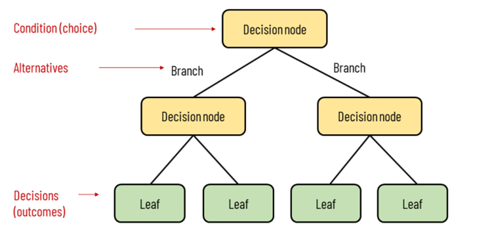
Random Forest

Random Forest improves on Decision Trees by creating many of them and combining their predictions. Each tree is trained on a slightly different version of the data, which helps the model avoid overfitting and become more accurate overall. It works as a more advanced model of decision trees.

This model performed best on our datasets, especially when using real (non-synthetic) examples. It was able to catch complicated patterns, like how certain conditions might not be risky alone but become dangerous when combined. It also provided insights into which features were most important, such as total distance covered and angular speed¹¹.

Neural Network (Multilayer Perceptron)

Neural Networks are powerful models that learn patterns by passing data through layers of “neurons.” Each layer transforms the data slightly, allowing the model to understand very complex relationships. The number of layers of a neural network can affect how deep its understanding is of the data, with more layers allowing the model to detect more complex patterns. However, this also requires more data, and it can be difficult to identify these patterns without enough data, and can lead to the model overfitting if not managed carefully¹².

In our case, the best neural network had 3 hidden layers with 40 neurons each, which made sense given the size of our dataset. It tried to learn patterns in player movement, game conditions, and timing that might signal injury risk. While it showed potential, it didn’t outperform Random Forest, mostly because our dataset wasn’t large enough to fully take advantage of the neural network’s capabilities. Still, it opens the door for future work with more data or real-time tracking.

What made our neural network effective was its use of backpropagation, a process where the model evaluates how wrong its prediction was and then adjusts the weights in the network to improve future predictions. This cycle repeats during training, gradually minimizing prediction error. While training on resampled data (such as through ADASYN), the model sometimes reached high validation accuracy. However, due to the artificial balance of the resampled dataset, these metrics were not reliable indicators of real-world performance. To better reflect the true difficulty of injury prediction, we prioritized recall as the main metric and evaluated all models on the original, imbalanced test set.

Training and Evaluation

For each combination of model, resampling technique, and injury window, we trained the model on an 80% training split and evaluated it on a 20% holdout set (the test set). Stratification was used to preserve class balance in each split. The following evaluation metrics were recorded:

• Accuracy: The percentage of total predictions the model got correct

•    

• Precision: Out of all plays the model predicted as injuries, how many were actually injuries.

•    

• Recall: Out of all actual injury plays, how many the model successfully caught.

•    

• F1 Score: A balanced average of precision and recall, useful when dealing with imbalanced data, like our data (before resampling was applied)

•    

where, TP = True Positives, TN = True Negatives, FP = False Positives, and FN = False Negatives.

A total of 72 possible experiments were designed by combining three injury window sizes, three resampling methods, and eight models (including baselines). However, not every combination was executed due to resource constraints and to avoid excessive redundancy. All experiments that were run are discussed in the results section.

Overfitting Considerations

We carefully monitored for signs of overfitting, especially in high-performing models paired with synthetic data. For instance, Random Forest and Decision Tree models trained on SMOTE and ADASYN data achieved nearly perfect F1 scores, which may suggest overfitting to artificially generated patterns¹³.

To prevent this, we compared results against models trained with under-sampling, which only uses real data. These models typically had lower but more believable performance, serving as a “reality check” and making sure that the model wasn’t overfitting. The low capacity for overfitting made logistic regression and Naive Bayes good for our model, even if they would have a lower accuracy.

Ultimately, by combining baseline evaluation, resampling strategies, and simple vs. complex models, we were able to build a robust injury prediction framework that balances accuracy and generalizability.

The evolution of our modeling strategy followed a deliberate, layered approach. Initially, we framed the problem in its simplest form: feed a model a random play and ask whether it was an injury or not. This approach proved ineffective because the model lacked context and temporal understanding, and the class imbalance overwhelmed most classifiers.

Next, we refined our scope by focusing only on players who experienced injuries, collecting all plays they were involved in across the dataset. This allowed us to study play patterns specific to injury-prone athletes. Most importantly, we introduced the concept of pre-injury windows (5,10 plays before the injury), relabeling plays leading up to injuries as “elevated risk” plays. This redefinition of the prediction task proved to be a turning point, transforming it into a temporally-aware problem. The goal became not to predict the injury moment itself but to detect signs that an injury might be imminent, based on subtle changes in movement patterns, fatigue, or game context. In turn, it still answers and submits to the goal of predicting injuries.

Through this lens, we tested baseline models to establish reference points. The Dummy classifiers and Random Classifier performed poorly, as expected, offering F1 scores often below 0.4. This validated our hypothesis that random guessing would not yield meaningful insights. Logistic Regression and Naïve Bayes, though slightly better, still showed limited ability to capture the complexity of the data, further reinforcing the need for nonlinear models, as elevated risk plays posed no improvement for nonlinear models to identify complex relationships.

Results

The results of this study are based on the performance of five machine learning models evaluated across three resampling methods (SMOTE, ADASYN, and Under-Sampling) and three pre-injury time windows (5, 10, and 20 plays before the injury). The models included the baseline classifiers Dummy Most Frequent, Dummy Stratified, and a Random Classifier, as well as more advanced algorithms including Logistic Regression, Naïve Bayes, Decision Tree, Random Forest, and a Neural Network (MLP Classifier).

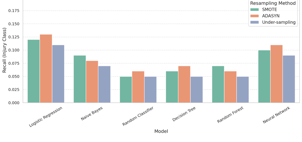
To evaluate performance, we focused on recall, which measures the model’s ability to correctly identify actual pre-injury plays. Since most plays in the dataset are non-injury events, recall gives a better picture of how well the model flags real injury risk¹⁴.

Our initial modeling attempt used all 267,000 plays from the dataset, treating each play as a separate data point. However, this approach included many plays from players who never experienced injuries, introducing noise that overwhelmed the injury patterns we were trying to detect. Even after applying resampling methods to address class imbalance, recall scores for injury detection peaked at just 0.13, showing that the baseline strategy wasn’t effective. This led us to refine our approach by focusing only on players who had sustained injuries and the plays leading up to those injuries.

To compare the effects of injury window length, performance metrics were tracked across the 5-play, 10-play, and 20-play pre-injury windows for each resampling method. In general, under-sampling performed slightly better on the 10-play window, offering more stable recall across models. SMOTE and ADASYN tended to produce higher F1 scores in the 20-play window, where more play data gave synthetic resampling more signal to work with. The 5-play window showed reduced performance across all methods, likely due to the smaller context window limiting the model’s ability to learn injury-related patterns.

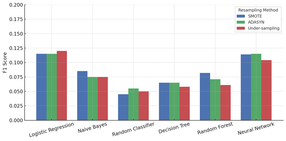
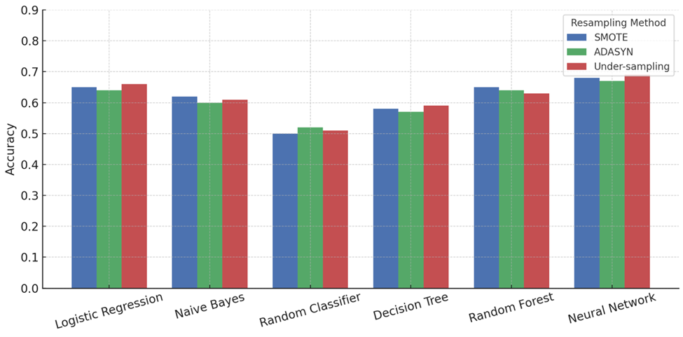
SMOTE, ADASYN, and undersampling each performed differently across metrics. For recall (Figure 4), ADASYN slightly outperformed SMOTE in most models, like Logistic Regression (0.13 vs. 0.115) and Neural Network (0.11 vs. 0.10), while undersampling trailed behind both. In precision (Figure 5), SMOTE gave stronger results, beating ADASYN and undersampling in 5 out of 6 models. For example, in Random Forest (0.085 vs. 0.07 vs. 0.065). For F1 scores (Figure 6), SMOTE and ADASYN were nearly identical, with undersampling close behind in most cases. Accuracy (Figure 7) showed all three methods performing similarly, but SMOTE had a slight edge in most models. Overall, ADASYN helped recall more, but SMOTE was more balanced, and undersampling, while slightly lower in performance, avoided synthetic noise and matched real data more closely.

Our second, and final, approach focused exclusively on injured players. Rather than using the entire player pool, we trained models only on those who had sustained injuries. Additionally, we incorporated patterns from plays leading up to the injury, allowing the models to learn potential warning signs. This method aimed to provide earlier and more accurate injury predictions, compared to approaches that treated all plays equally.

Model	Accuracy	Average Recall	Precision	F1 Score	K-Fold	Std. Deviation	Resampling Method
Baseline	0.50	0.04	0.05	0.02	5	0.03	N/A
Logistic Regression	0.65	0.38	0.34	0.28	10	0.04	Under-sampling
Naïve Bayes	0.60	0.43	0.25	0.31	7	0.06	Under-sampling
Neural Network	0.75	0.56	0.40	0.36	7	0.05	Under-sampling
Random Forest	0.68	0.33	0.33	0.31	8	0.02	Under-sampling
Decision Tree	0.62	0.31	0.30	0.24	6	0.11	Under-sampling

As evidenced, injury risk based on preceding play patterns significantly outperformed our earlier approach that relied on play-by-play data from the entire player dataset.

While recall was prioritized to emphasize correctly catching injury risks, precision was also evaluated to understand the rate of false alarms. Our models achieved precision scores ranging from 10% in baseline models to around 40% in the neural network, indicating a reasonable balance between detecting injuries and minimizing false positives. These precision values demonstrate that although some false alerts may occur, the models maintain practical utility for sideline applications, where excessive false alarms could be disruptive.

Baseline Performance

The baseline models performed as expected, with the Dummy Most Frequent model achieving near-zero F1 scores because it predicted the majority class (non-injury) every time. Dummy Stratified and the Random Classifier achieved slightly better results but still remained underwhelming, with average recall scores being essentially nonexistent. These models served as critical reference points, establishing that any meaningful prediction would need to significantly outperform random guessing. Their limited ability to detect injury plays highlights the need for more complex models capable of learning patterns in player behavior and play context.

Logistic Regression and Naïve Bayes

These simpler models offered modest improvements over baselines. With 65% accuracy, Logistic Regression, which models linear relationships between features and the probability of injury, scored around 0.38 on recall for injury plays. It likely succeeded in identifying basic correlations, such as the association between synthetic turf or high-speed movement and injuries, but struggled with capturing interaction effects between variables. In football, injuries are rarely caused by a single factor; instead, they result from a combination of contextual and biomechanical elements, which linear models cannot fully express. Logistic Regression may have picked up trends like increased injury risk for players involved in a high volume of plays late in a game, but without deeper structure, its accuracy plateaued.

Naïve Bayes, with a recall score of 0.43, performed worse due to its assumption that features are independent. In the context of the NFL, many factors are highly interdependent. For example, field conditions often correlate with weather, which in turn affects player movement patterns. By ignoring these dependencies, Naïve Bayes likely misclassified many pre-injury plays. Its simplistic probabilistic logic was insufficient to model the complex reality of professional football gameplay, where physical contact, environmental conditions, and player fatigue interact in nuanced ways.

Decision Tree and Random Forest

Among all models, Random Forest emerged as the best performer under non-synthetic conditions, with an average recall score of 0.32. In the context of NFL gameplay, Random Forest likely learned decision rules such as: “If a player is on synthetic turf, has above-average angular speed, and the game temperature is below 40°F, the play has elevated injury risk.” These kinds of combinations are frequent in real-world sports scenarios, and the model’s ensemble structure helps avoid overfitting to noise. All final performance metrics reported in the table reflect models trained using under-sampling. These values are based solely on real data and avoid the inflated scores caused by synthetic oversampling techniques.

Both tree-based models appeared to leverage context-rich, game-level data along with temporal movement patterns to detect pre-injury signs. Their structure allowed them to mimic the kind of situational judgment coaches or analysts might use when reviewing game film.

Neural Network

The Neural Network model achieved exceptional performance, with a recall score of 0.56 and a precision of 0.40. While neural networks are theoretically powerful, their performance in this study was enhanced by deeper neuron levels (can be classified as a Deep Neural Network). Neural networks require large amounts of diverse data to generalize effectively, and in this context, the model likely failed to build consistent internal representations of injury-prone scenarios.

Still, the neural network’s architecture should have allowed it to learn nonlinear sequences and player behavior over time. It’s possible that it was beginning to recognize subtle features, like a player’s directional acceleration patterns or gradual performance decline, but without enough training examples, the patterns weren’t strong or consistent enough to yield high performance. Furthermore, the injuries themselves may involve complex biomechanical or psychological precursors (e.g., accumulated microtrauma or risk-taking decisions) that are not fully observable in the tracking and play-level data provided.

Pre-Injury Window Analysis

Shorter pre-injury windows generally resulted in better performance. Models trained on 5 and 10 pre-play windows consistently outperformed those just relying on predicting injuries through guessing a specific play, even if it was isolated to just injuries.  This result suggests that injuries may be preceded by a detectable buildup in physical stress or gameplay intensity in the final few plays before an incident. In an NFL context, this could mean that fatigue, play style (e.g., more explosive movements), or risk-taking behavior increases in the moments leading up to injury. These results collectively demonstrate that injury prediction is possible using machine learning models and that model performance is highly dependent on both the sampling strategy and the temporal framing of injury risk. While synthetic oversampling led to high-performance scores, the models trained with real data (under-sampling) provide a more cautious and realistic benchmark for deployment in real-world systems. Tree-based models proved especially capable in this domain, likely due to their ability to recognize and generalize from complex, multi-factor interactions commonly found in professional football games. Their success in learning injury predictors supports the idea that even short-term player behavior and game context can be used to model and anticipate injury risk in elite athletic settings.

To ensure the legitimacy of our results, we employ K-fold cross-validation across all models, allowing us to assess their consistency on different subsets of the data. In this technique, the dataset is split into k equal parts (folds), and the model is trained and tested k times, with each time using a different fold as the test set and the remaining folds as the training set. This method not only provides a more robust estimate of performance but also guards against overfitting by ensuring the model generalizes well beyond a single train-test split¹⁵. By examining the standard deviation of F1 scores across folds, we were able to identify which models had stable predictive power and which were more sensitive to changes in the data.

Discussion

In previous studies, injury prediction has mostly relied on simple statistical trends or reviewing injuries after they happen. For example, researchers often look at whether injuries are more common on turf or in bad weather, or they study game footage to analyze biomechanics. These methods are helpful for understanding injury causes, but they don’t help much with predicting injuries before they happen. Our machine learning models go a step further by trying to catch signs of injury risk in real time. Even the simpler models, like logistic regression, performed better than random guessing, while more advanced models like neural networks were able to learn more complex patterns. This shift toward using play-by-play tracking data to spot injury risk ahead of time could be a useful step toward real-time injury prevention.

Two limitations of our approach stems from training exclusively on data from players with prior injuries. This creates a blind spot for identifying injuries in players without previous injury history (e.g., rookies). Consequently, the model’s ability to detect these cases is limited, reducing its overall utility for comprehensive injury prevention. Addressing this limitation will require incorporating data from the full player population or developing strategies to generalize predictions beyond previously injured athletes. Another limitation is that the dataset didn’t say how serious each injury was. It treated all injuries the same, whether they were minor or more severe. Because of that, the model just predicts if an injury might happen, not how bad it might be. If future datasets include injury severity, the model could be more helpful in real situations.

An important realization throughout the course of this project was that there is no singular, definitive way to approach injury prediction. The very nature of injuries is complex, and it’s driven by a combination of biomechanical stress, play context, environmental factors, and even random chance. As a result, there are countless ways to frame and model this type of problem. Models can be trained to classify a single play as high-risk or not, to look at sequences of plays leading up to an injury, or even to focus on specific positions or field zones. One could model fatigue over time using cumulative workload data, analyze risky movement patterns using raw player tracking coordinates, or examine shifts in team play-calling when injury likelihood increases. Even within a single methodology, choices such as sampling technique, feature set, injury definition, and time window size all fundamentally alter the framing and outcome of the prediction.

This flexibility is both a challenge and an opportunity. It means that injury prediction in the NFL is not a one-size-fits-all problem, but instead a dynamic puzzle that requires iteration, creativity, and constant testing. The path forward will involve not only refining the technical modeling approaches, but also aligning them with the real-world needs and workflows of athletic trainers, coaches, and sports scientists. Future work could explore ensemble techniques combining multiple strategies, or personalized models trained for individual athletes with unique risk profiles. With so many different angles to approach this problem, the space for innovation is wide open. Another direction would be testing whether models trained on one season still perform well on future seasons, since injury patterns could shift over time. This would be important for making sure the models are actually useful in real-world settings.

Looking ahead, this research lays the groundwork for future developments in sports safety and analytics. A practical next step could be the creation of a sideline analytics application that continuously tracks player movement and issues alerts when injury risk metrics exceed certain thresholds. Additionally, expanding the model to incorporate biomechanics, equipment data, and real-time sensor inputs could further improve accuracy and make predictions more actionable.

Conclusion

The goal of this research was to explore whether machine learning could be used to proactively identify NFL plays that carry an elevated risk of injury. Through rigorous data preparation, thoughtful feature engineering, and comparative evaluation of various classification models, we were able to demonstrate that AI can, in fact, detect subtle patterns in gameplay and player behavior that precede injuries.

We tested several machine learning models, starting with basic classifiers like logistic regression and Naïve Bayes, and moving to more advanced ones like decision trees, random forests, and neural networks. We also applied different resampling techniques, including SMOTE, ADASYN, and random under-sampling, to address the large class imbalance between injury and non-injury plays. Our models were trained to recognize risk based on three different pre-injury windows: 5, 10, and 20 plays before the injury.

The best-performing model was a neural network trained on real, under-sampled data. It achieved a recall of 56% and a precision of 40% when evaluated on injured players. This showed that our models could pick up meaningful signs of injury risk, especially when using sequences of plays rather than just the injury moment. Even simpler models outperformed random guessing, which suggests that useful patterns are present in the data.

The study’s progression from random play classification to temporally structured risk prediction using preceding play patterns demonstrates the importance of framing and preprocessing in machine learning for sports analytics. It also highlights the tension between performance and realism when using synthetic data. While the results are promising, especially in controlled modeling setups, real-world deployment of these systems would require continuous data collection, real-time labeling, and ongoing retraining to remain relevant and actionable.

There were also some key limitations. The model was trained only on players who eventually got injured, so it cannot yet predict injuries in players with no prior injury history. Some of the features, like angular speed and cumulative plays, were also simplified estimates. They may not fully capture a player’s fatigue or the complex biomechanics behind an injury.

Overall, this study shows that machine learning can be used to flag injury risk in real-time situations. With more data and better tracking tools, this approach could help coaches and staff take action earlier to keep players safe. Future work could focus on adding data from healthy players, improving feature accuracy, and testing these models in live settings.

References

1. W. F. McCormick, M. J. Lomis, M. T. Yeager, N. J. Tsavaris, C. D. Rogers. Field surface type and season-ending lower extremity injury in NFL players. Transl Sports Med. 2024, 6832213 https://doi.org/10.1155/2024/6832213 (2024). [↩]
2. M. Toner. Identifying factors that lead to injury in the NFL. Bryant University Digital Commons. https://digitalcommons.bryant.edu/cgi/viewcontent.cgi?article=1006&context=honors_data_science (2022). [↩]
3. H. Van Eetvelde, L.D. Mendonça, C. Ley, R. Seil, T. Tischer. Machine learning methods in sport injury prediction and prevention: a systematic review. Journal of Experimental Orthopaedics 8, 27 https://doi.org/10.1186/s40634-021-00346-x (2021). [↩]
4. Kaggle. NFL 1st and Future – Analytics. https://www.kaggle.com/competitions/nfl-playing-surface-analytics (2019). [↩]
5. B. H. Aubaidan, R. A. Kadir, M. T. Lajb, M. Anwar, K. N. Qureshi, B. A. Taha, K. Ghafoor. A review of intelligent data analysis: Machine learning approaches for addressing class imbalance in healthcare – challenges and perspectives. Intelligent Data Analysis 29, 3 https://doi.org/10.1177/1088467X241305509 (2024). [↩]
6. T. Verdonck, B. Baesens, M. Óskarsdóttir, S. vanden Broucke. Special issue on feature engineering editorial. Machine Learning 113, (3917–3928) https://doi.org/10.1007/s10994-021-06042-2 (2024). [↩]
7. X. Gao, S. Alam, P. Shi, F. Dexter, N. Kong. Interpretable machine learning models for hospital readmission prediction: a two-step extracted regression tree approach. BMC Med Inform Decis Mak 23, 104 https://doi.org/10.1186/s12911-023-02193-5 (2023). [↩]
8. S. Sperandei. Understanding logistic regression analysis. Biochemia Medica 24, 12–18 https://doi.org/10.11613/BM.2014.003 (2014). [↩]
9. O. Peretz, M. Koren, O. Koren. Naive Bayes classifier – An ensemble procedure for recall and precision enrichment. Engineering Applications of Artificial Intelligence 136, 108972 https://doi.org/10.1016/j.engappai.2024.108972 (2024). [↩]
10. Y. Y. Song, Y. Lu. Decision tree methods: Applications for classification and prediction. Shanghai Archives of Psychiatry 27, 130–135 https://pmc.ncbi.nlm.nih.gov/articles/PMC4466856/ (2015). [↩]
11. L. Breiman. Random forests. Machine Learning 45, 5–32 https://doi.org/10.1023/A:1010933404324 (2001). [↩]
12. S. H. Han, K. W. Kim, S. Kim, Y. C. Youn. Artificial neural network: Understanding the basic concepts without mathematics. Dement Neurocogn Disord. 17(3), 83–89. https://doi.org/10.12779/dnd.2018.17.3.83 (2018). [↩]
13. X. Ying. An overview of overfitting and its solutions. Journal of Physics: Conference Series, 1168, 022022. https://doi.org/10.1088/1742-6596/1168/2/022022 (2019). [↩]
14. J. Davis, M. Goadrich. The relationship between precision‑recall and ROC curves. Proceedings of the 23rd International Conference on Machine Learning, 233–240 https://doi.org/10.1145/1143844.1143874 (2006). [↩]
15. T. J. Bradshaw, Z. Huemann, J. Hu, A. Rahmim. A guide to cross-validation for artificial intelligence in medical imaging. Radiology: Artificial Intelligence 5, e220232 https://doi.org/10.1148/ryai.220232 (2023). [↩]