
Abstract
Despite the consequence of species going extinct not currently being visible, its impact in our future can be devastating to biodiversity, ecosystem stability, and our own society. Predicting extinction rates and identifying the primary causes of a species decline are crucial first steps to improving our conservation efforts. An accurate understanding and insight into factors driving species extinction can equip conservationists with the tools needed to preserve endangered species. As the number of extinct species continues to rise, a variety of issues become apparent. As species decline, so does biodiversity. With reduced biodiversity, many species – and by extension humans – could suffer from reduced resilience, causing us to be more easily influenced by diseases and climate change.To protect species at risk of extinction, conservationists need to identify which species are most vulnerable by understanding the factors that drive their decline. Utilizing AI models is a crucial first step in this process. This study utilizes the Random Forest Regressor model, trained on “Animal Information Dataset” published on Kaggle containing characteristics across a range of species, to help conservationists understand which species are at a greater risk of extinction1. To ensure robustness, our model was tested using k-fold cross-validation to calculate RMSE values, such as those for the Amur Tiger and Alaotra Grebe being 2.94 and 8.85 years respectively. The model provides a relative timeline for species decline, allowing conservationists to more strategically allocate their resources. This paper explores the development of a prediction model designed to predict extinction rates, ultimately aiding conservationists in their efforts to protect endangered species.
Introduction
The decline and eventual extinction of species has become a major issue in modern times. A variety of species have gone extinct recently; some such species being the Alaotra Grebe which went extinct back in 2012, the Bramble Cay Melomys in 2016, and the Maui Akepa in 20182,3,4.
The permanent loss of species can lead to ecosystem destruction which can cause irreversible damage to our planet and negatively impact our lives. Due to the structure of ecosystems, every species has a role to play, such as in food production and resource accessibility, making their extinction have a direct negative impact on us.
When a species goes extinct, they cause an imbalance in the food chain5. The predators that used to consume them now have a reduced food source, which could lead to their starvation. Without natural predators, prey can grow uncontrollably, leading to imbalances in the ecosystem. As the number of species declines, so does biodiversity5. With reduced biodiversity, many species – and humans – could suffer from reduced resilience, causing us to be more easily influenced by diseases and climate change.
Some human-induced extinction factors include climate change, pollution, and changes in habitat6. Understanding these factors is key to understanding extinction events. Not all extinction factors are man-made, yet people can still mitigate their effects. For example, an abundance of predators, a lack of resources, or the inability to reproduce all play significant roles, and are a few examples of natural extinction causes.
Many modern prediction models related to extinction prediction focus mainly on a very specific species7. An underworked part of extinction prediction models is creating a general model that could give extinction dates for a variety of animals. Unlike standard extinction prediction models that focus on a single species, this model uses a multi-species dataset to predict extinctions across a wider taxonomic range.
Related Works
Comparative studies have shown species traits can be associated with extinction risk6. Across taxa, characteristics such as offspring production, taxonomic group, and social group size have correlations with extinction risk8. These results helped narrow down our search for datasets when deciding on characteristics to utilize for training the model.
Knowing this, past research has been done to approximate the International Union for Conservation and Nature (IUCN) Red Lists threat categories for species that are Data Deficient7,9. Approaches typically tend to combine traits to identify species that are most at risk, using feature importance to drive their predictions7,10.
This paper seeks to follow trait-based ML predictions but in a different way: developing a general species extinction prediction model to predict lifespans rather than IUCN statuses11.
Methods
To predict the extinction date of species, there are several key steps. Firstly, identifying the best type of model for the most accurate prediction. Next, collecting proper data to make accurate predictions. Lastly, training the model on the data to predict their relative extinction date.
To decide on the best type of model, a variety of different models were researched to better understand their pros, cons, and varying use cases. After understanding multiple different models such as XGBoost, K-Nearest Neighbors (KNN), and Linear Regression, the model that was chosen for this research was the Random Forest Regressor model12,13.
Unlike some of the previously mentioned models, Random Forest Regressor excels at handling smaller amounts of data, whereas Linear Regression which might underfit due to its simplicity or XGBoost which can overfit due to recognizing quirks rather than general patterns12,14. In addition, it excels at handling large amounts of categorical data where other models such as Linear Regression and KNN struggle12,15. Finally, due to its use of multiple decision trees, it is able to more easily simulate complex ecological relationships by better accounting for various characteristic combinations compared to other model types.
In short, RandomForestRegressor splits testing data into several decision trees, unlike other models that just rely on one decision tree. By using multiple decision trees and comparing them to one another, the model enhances its ability to make accurate predictions12. Then, when the model is supplied with data, it can compare the input data with the preprocessed data to find patterns to make predictions of the expected outcome.
To make predictions, adequate data on the topic is needed. After extensive searching, we selected the dataset, “Animal Information Dataset,” published by Sourav Banerjee on Kaggle, an online platform used for data science competitions that simultaneously hosts a large library of free use data. This specific dataset was chosen as it contained 16 characteristics spanning 206 species which would allow the model to be usable in a general setting. The dataset spans a wide range of taxa – such as mammals, reptiles, birds, and aquatic species – allowing the model to train on a diverse set of ecological traits. However, a majority of the data have lifespans under 30 years which could overrepresent short-lived species.
The data is often unusable in its base form, as it is not tailored towards the model. As such, preprocessing the data is required.
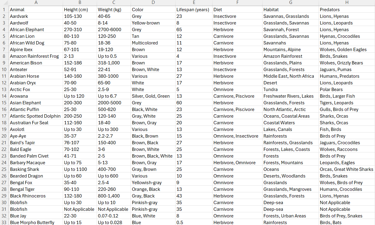
In the end, the columns that remained, which represent the training characteristics, were Animal, Height (cm), Weight (kg), Color, Lifespan (years), Diet, Habitat, Predators, Average Speed (km/h), Countries Found, Conservation Status, Family, Gestation Period (days), Top Speed (km/h), Social Structure, and Offspring per Birth. These characteristics can be found in Figure 1. The model utilizes these combined characteristics to formulate accurate predictions. In addition to removing certain unnecessary columns, minor edits to the data were necessary to ensure usability such as removing hyphens for certain characteristics, changing capitalization, and other small data fixes. Feature engineering steps were taken to remove all null values from the data, re-format categorical inputs (e.g. ‘USA’ and ‘US’), and apply one-hot encoding to avoid ranking categorical data in a similar style to numerical values16,17. When using data to make predictions, it is also important to classify pieces of data as numerical or categorical.
Numerical is data that uses numbers (integers & floats), while categorical uses words (strings). The model must know which characteristics use numerical and categorical, as the model treats them differently when making predictions. Numerical data can be compared much more easily, as the model can easily compare different numbers to each other. Since the model used in this research was Random Forest Regressor, which utilizes decision trees which are not sensitive to feature magnitude, no feature scaling was used12.
Scikit-learn version: 1.6.1 was used with the default hyperparameters, some of which included n_estimators: 100 (number of trees), criterion: ‘squared_error’ (how splits are evaluated), min_samples_split: 2 (minimum samples needed to split a node), and many others16. While this study did not focus on hyperparameter tuning due to the purpose of the research being to identify the feasibility of a general extinction prediction model, future work could explore optimizing these values to further improve accuracy in the model’s predictions.
Categorical data is treated differently as words cannot be compared with one another the same way numbers can. Assigning numerical values to countries could help improve accuracy. For example, assigning the US and USA the value of 1 can help to classify the United States of America as just one piece of data, rather than two pieces of data, as in categorical terms, the US and USA would act as different values despite meaning the same thing. Accurately classifying data as numerical and categorical before running the model can significantly boost the model’s accuracy. In this study, one-hot encoding was utilized to prevent the implicit ranking of categories.
Not all the data is used to train the model. The data is split into a training and testing category. By using all the data on training, the prediction model may be too rigid, and struggle making predictions when the input data is not what is directly from the training data. This is known as overfitting and can lead to very inaccurate predictions due to the model not being flexible enough to make accurate predictions. Underfitting, on the other hand, works in the opposite way. Using too little training data can cause the pattern recognition to be weak, causing the model’s accuracy to suffer. The most common train-test splits are 80% train and 20% test, 67% train and 33% test, and 50% train and 50% test18.
Finding a balance between splitting the training and testing data is key to accuracy and consistency of the model. When running the model, the model trains using the training data, and then tries making predictions using the testing data, checking its predictions with the actual values of the testing data. To make predictions of species expected extinction dates, there are a series of steps that need to be taken. Firstly, it is necessary to separate the characteristics into X and Y datasets.
The Y represents what information that is being predicted, and in this case, the lifespan of the species, as that can be used to predict extinction dates using basic math. The rest of the characteristics mentioned earlier were put into the X list.
As previously mentioned, the X and Y datasets were split into training and testing data. After testing the model, a split of 80% training data and 20% testing data worked best for this specific experiment when trying to make accurate predictions. Then the training data is used to fit the model, causing the model to learn about the data and create the patterns mentioned earlier. Now, when inputting new data (all characteristics mentioned earlier excluding lifespan) about animals not previously in the dataset, the model can recognize patterns in the data to give estimations about expected lifespans of certain species. With the predicted lifespan, the following information can be calculated:
- 𝐷𝑒𝑎𝑡ℎ𝑠 𝑃𝑒𝑟 𝑌𝑒𝑎𝑟 = Population / Lifespan
- 𝐵𝑖𝑟𝑡ℎ𝑠 𝑃𝑒𝑟 𝑌𝑒𝑎𝑟 = 𝑂𝑓𝑓𝑠𝑝𝑟𝑖𝑛𝑔 𝑃𝑒𝑟 𝐵𝑖𝑟𝑡ℎ * # 𝑜𝑓 𝑇𝑖𝑚𝑒𝑠 𝑅𝑒𝑝𝑟𝑜𝑑𝑢𝑐𝑖𝑛𝑔 𝑃𝑒𝑟 𝑌𝑒𝑎𝑟
- 𝑅𝑎𝑡𝑒 𝑜𝑓 𝐶ℎ𝑎𝑛𝑔𝑒 𝑜𝑓 𝑡ℎ𝑒 𝑃𝑜𝑝𝑢𝑙𝑎𝑡𝑖𝑜𝑛 𝑜𝑓 𝑆𝑝𝑒𝑐𝑖𝑒𝑠 = 𝐵𝑖𝑟𝑡ℎ𝑠 𝑃𝑒𝑟 𝑌𝑒𝑎𝑟 − 𝐷𝑒𝑎𝑡ℎ𝑠 𝑃𝑒𝑟 𝑌𝑒𝑎𝑟
With this information, it is possible to graph an exponential equation which can represent the population of species by using the equation
𝐹𝑢𝑡𝑢𝑟𝑒 𝑃𝑜𝑝𝑢𝑙𝑎𝑡𝑖𝑜𝑛 = 𝐶𝑢𝑟𝑟𝑒𝑛𝑡 𝑃𝑜𝑝𝑢𝑙𝑎𝑡𝑖𝑜𝑛 * 𝐺𝑟𝑜𝑤𝑡ℎ 𝑅𝑎𝑡𝑒𝑇𝑖𝑚𝑒
where the X-axis represents time and the Y-axis represents the population.
There are two methods that can be employed to check for accuracy of the model, checking the root mean squared error (RMSE) or the R-squared value.
The mean squared error is a way of quantifying the overall error of the model. To do this, it averages the squared differences between the predicted and actual values of the model. By utilizing sklearn’s cross_val_score function, we were able to calculate the RMSE value for both species. This was done by performing 10-fold cross-validation and computing the negative mean squared average for each fold, before averaging those results and taking the square root to obtain the RMSE16,18,19,20. For the Amur Tigers and Alaotra Grebe graphs that are shown in the Results section of this paper, the RMSE values of 2.94 and 8.85 were obtained respectively. Considering the lifespan range in the dataset spanned from 0.25 to 125 years, an error of 2.94 and 8.85 years is a relatively small portion of the total range. This suggests that the model performs well when predicting species lifespans.
The R-squared (R2) value measures the amount of error that can be explained by the independent variables21. By using scikit-learn’s r2_score function, the R2 value was calculated as one minus the sum of squared differences between the predicted and actual values divided by the sum of the squared differences between actual values and their mean. An R2 value closer to 1 shows that the model accounts for a greater variance in the data, while a value closer to 0 shows that the model performs the same as predicting the mean. For the Amur Tiger and Alaotra Grebe, they got an R2 of 0.84 (83.76%) and 0.85 (84.67%) respectively. This signifies that in both cases, the model explains over 83% of the variation in lifespan, demonstrating a strong prediction.
Since the RMSE and R2 values highly depend on the training data, prediction parameters, and range of values, comparing them across models can be misleading. As such, a direct comparison between these values was avoided in this study21.
Results
To test the Random Forest Regressor model, the extinction dates of multiple species were predicted to test for accuracy and validity.
The Amur Tiger (otherwise known as the Siberian Tiger) is a species of tiger that is currently critically endangered.

Based on prediction trends, the Amur Tigers were expected to go extinct around the year 2055 as shown in Figure 2. Due to the graph’s exponential shape when relating time and population, the population numbers will never reach 0. However, estimations can be made on when species may go extinct based on how low their populations become. Based on all the tested characteristics being input to the model, the Amur Tigers are predicted to go extinct around that time frame, unless major action gets taken to support them. To validate these findings, two series of tests were run.
The first test took the Amur Tigers population from 15 years ago, and tried to predict its current population, assuming none of the factors affecting their growth or decline changed.

This graph shows that by following the trend of their population 15 years ago (325 Amur Tigers), a prediction can be made for the present day: there should be roughly 100 tigers left.
The second test tried to predict the rough extinction date of an already extinct species. To do this, a prediction was made for the Alaotra Grebe, a species of bird which unfortunately went extinct in 2012.

Their population from 50 years ago was taken and used to predict their population to find when they may go extinct. Based on the exponential curve, a safe prediction is that their species may go extinct around 2015, as that is when their population numbers become dangerously low. With their actual date of extinction matching the predicted extinction, it is safe to assume that the model is relatively accurate when predicting extinction risk of species.
Luckily for Amur Tigers, Russia has been making conservation efforts to increase their population. Russia’s efforts have been effective, as in recent times, the Amur Tiger population has been steadily increasing. However, if Russia did not take the appropriate measures to maintain the tiger’s safety, these graphs reveal some potential scenarios that could have taken place. Figures 5 – 8 show example graphs of various species’ predicted population over time graphs.

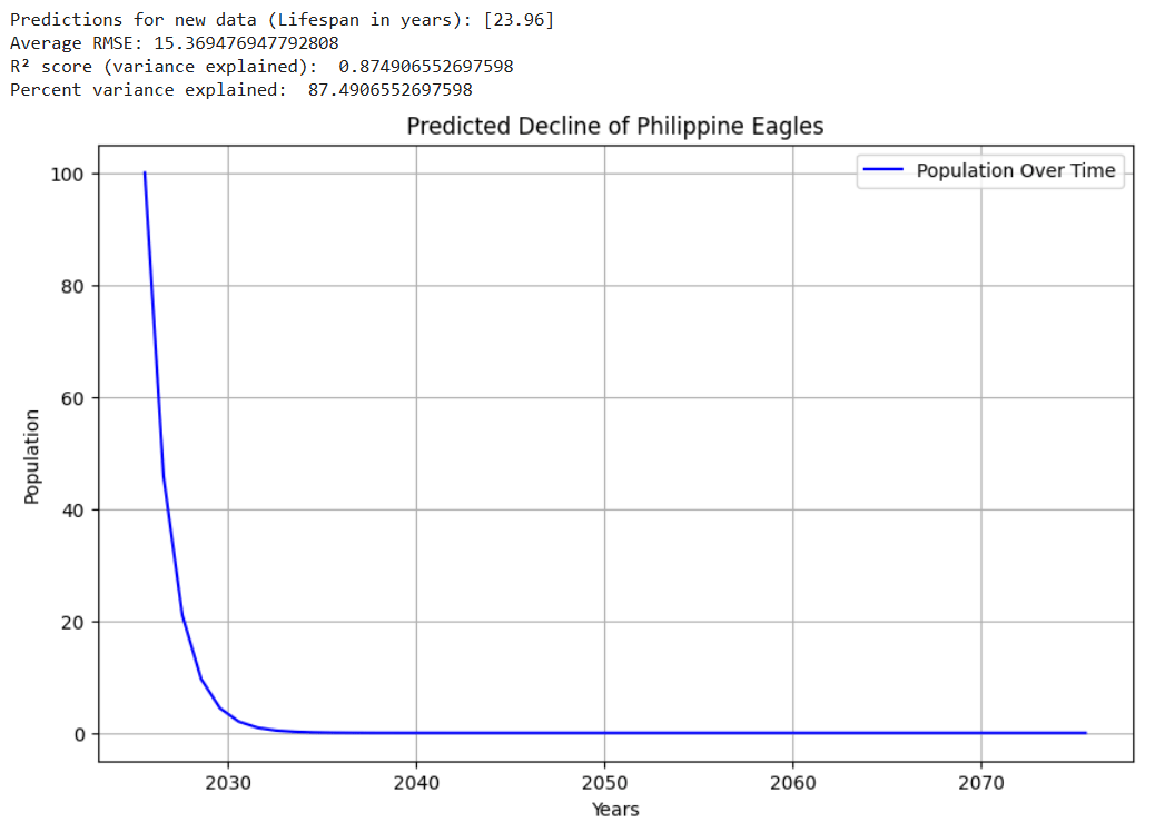

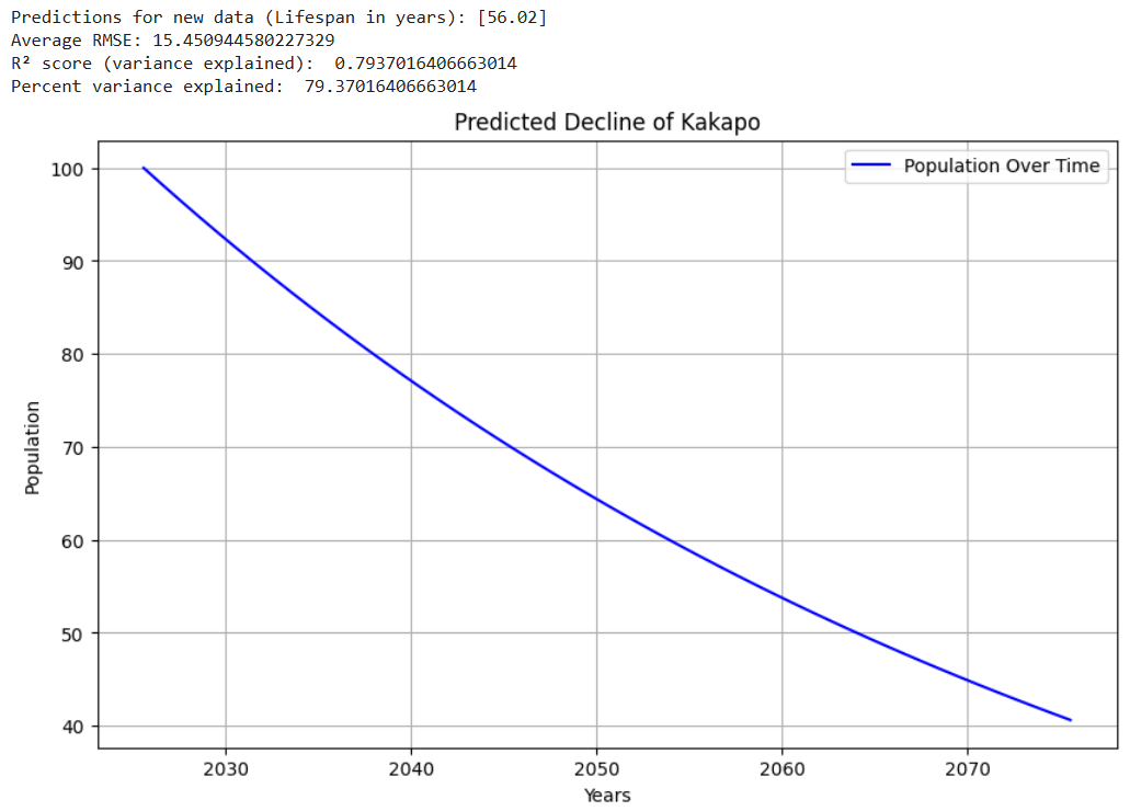
Figure 8. Graph showing predicted decline of the Kakapo16,26(lifespan : ~60)
In addition, understanding the factors behind species extinction is equally as important as understanding relative extinction dates. While analyzing the driving factors that led to reduced populations, feature importance revealed how the species family (e.g. Elephantidae, Felidae, Canidae, etc.), number of offspring per birth, and color were the strongest characteristics that drove extinction27. In contrast, traits such as social structure (solitary, herd-based, or group-based), top speed, and average speed had minimal effects relative to other characteristics when determining overall population extinction11,28. These results suggest that ecological and reproductive factors play a more critical role than raw physical or behavioral traits in determining species survival.
While some features may be biologically important in survival such as social structure or speed, due to those traits showing reduced relative importance in this dataset, it may imply that there may be limitations in the data rather than those characteristics true ecological role.
Discussion
This research showcases the feasibility of a general prediction model, specifically Random Forest Regressor, to predict extinction risk across a diverse range of species. The model’s alignment with both historical extinction (e.g. Alaotra Grebe) and future risk species (e.g. Amur Tiger) suggests accurate predictive findings.
The consistency between the model’s predictions and real world conservation efforts (e.g. Russia’s emphasis on Amur Tiger conservation) support the model’s accuracy. However, these results suggest correlations between characteristics and extinction risk and are not meant to be used without proper ecological expertise. Additionally, the model’s ability to predict across taxa is promising, but species-specific traits and unique ecological dynamics can still cause significant predictive error10,29.
While the model itself showcases reasonable accuracy in predicting the extinction date of species, it is difficult to compare it to a species-specific model as they serve distinct purposes. A species-specific model is specialized for a single organism and can produce higher accuracy predictions at the cost of time. A general model such as this one, on the other hand, can significantly reduce the time taken to make predictions on a wide range of taxa, allowing for better scalability, at the cost of reduced accuracy.
However, despite the model being accurate for many species, there are still several limitations that should be considered. One main factor is the variability in species ecosystem interactions. While the model does incorporate multiple biological factors such as reproductive rate, diet, and social structure, some species have unique biological responses that may potentially influence its extinction path in ways that may not be captured by the model. The model might oversimplify or completely omit crucial interactions between species, food accessibility, or disease prevalence which can vary widely even within a single habitat.
Additionally, the availability of data also posed serious limitations. Due to the limited data available to use, the model was most accurate when predicting the lifespan and extinction date of species with certain traits. When binned by lifespan, species with short lifespans (under 30 years) had a mean absolute error (MAE) of 1.21-1.53 but increased to 2.06 for species between ages 30 and 60 and increasing all the way to 7.01 for lifespans greater than 60 years. When creating bins based on conservation status, (e.g., least concern, critically endangered, etc.) the MAE was lower (0.96) when predicting species in more common categories (least concern) when compared to those in threatened categories (e.g. Endangered: 2.25 or Vulnerable: 2.49). Many of these skews in prediction accuracy can most likely be attributed to the dataset having more available species in those specific categories, allowing for stronger predictions in those areas.
Finally, due to the model having a set number of factors it is checking for and using to make predictions, it is difficult to account for unforeseen variables such as the impact of conservation areas, habitat loss/expansion, or natural disasters.
The potential impact of these findings can be used to highlight the role of predictive modeling in conservation biology. The ability to anticipate extinction timelines for species allows for preemptive action. By utilizing the insight of machine learning models, resources can be better allocated to more effectively and efficiently support species when needed. Models such as this one can add a data-driven perspective that complements conservationists expertise, helping to identify species that may experience rapid population declines without the proper support.
This study’s model functions as an early warning system rather than a surefire predictor on species extinction risk. This model can act as a tool for biologists to use, complementing conservationists skills to better understand extinction trends. The predictive data generated can support the hypothesis that certain species are at a high risk of extinction.
There are a few improvements that could be made to this project. Keeping track of more recent environmental impacts would greatly increase the accuracy of the prediction results. By incorporating factors relating to human impact such as global warming, pollution, and other modern factors, the results could be greatly influenced. With the increase in characteristics, the model would become more complex. In return, it would have increased accuracy as the model would be able to recognize patterns in the data more easily. By including additional factors, the model can better reflect the complex intricacies of modern environmental issues.
Additionally, being able to link the predictions with real time systems such as satellite data could be used to make more dynamic predictions. By accounting for current weather conditions, changes in environments due to – deforestation, temperature rises, and increased sea levels – as well as monitoring the effect of protected areas (such as national parks, nature reserves, and wildlife sanctuaries) versus non-protected areas (wilderness), the real time systems would allow conservationists to immediately react to environmental changes.
As shown by the data, it is possible to create a general model that can predict the lifespans, population, and extinction risk of species. It was possible to decide which model was the most effective by running practice simulations and testing. By training the model with data that was preprocessed, predictions were made on the lifespan, population numbers, and extinction risk of declining species. Finally, it was possible to cross-check the work by running an additional series of tests to validate the findings.
This research may prove beneficial to conservationists, as they can better allocate their conservation efforts to species that have a greater risk of extinction soon, allowing a more effective conservation effort regarding endangered species. As most modern prediction models are hyper-focused on a specific species in a small sub-region on the globe, this model strives to give an accurate, and more general, prediction for any species. Due to the current dataset having such limited information, the predictions for lifespans may not always be accurate, especially when species lifespans are too long or too short, as the current dataset does not have enough species with lifespans in those ranges to use as training data. As a result, when the model tries to run a simulation, the outcomes may be different than expected which could lead to inconsistencies while predicting extinction risk.
Appendix
Github Link: https://github.com/YogithKishore/ExtinctionPrediction.git
References
- “Animal Information Dataset.” Kaggle, 20 Sept. (2023), www.kaggle.com/datasets/iamsouravbanerjee/animal-information-dataset. [↩]
- BirdLife International (BirdLife International). “IUCN Red List of Threatened Species: Tachybaptus Rufolavatus.” IUCN Red List of Threatened Species, 10 Nov. (2022), www.iucnredlist.org/species/22696558/208158571. [↩]
- Arts, John Woinarski Resources Environment And. “IUCN Red List of Threatened Species: Melomys rubicola.” IUCN Red List of Threatened Species, (2025), www.iucnredlist.org/species/13132/254623401. [↩]
- BirdLife International (BirdLife International). “IUCN Red List of Threatened Species: Loxops Ochraceus.” IUCN Red List of Threatened Species, 26 Feb. (2024), www.iucnredlist.org/species/103824084/250520617. [↩]
- Wearn, Oliver R., et al. “Extinction Debt and Windows of Conservation Opportunity in the Brazilian Amazon.” Science, vol. 337, no. 6091, July (2012), pp. 228–32, doi:10.1126/science.1219013. [↩] [↩]
- Davidson, Ana D., et al. “Drivers and Hotspots of Extinction Risk in Marine Mammals.” Proceedings of the National Academy of Sciences, vol. 109, no. 9, Jan. (2012), pp. 3395–400, doi:10.1073/pnas.1121469109. [↩] [↩]
- Howard, Sam D., and David P. Bickford. “Amphibians Over the Edge: Silent Extinction Risk of Data Deficient Species.” Diversity and Distributions, vol. 20, no. 7, May (2014), pp. 837–46, doi:10.1111/ddi.12218. [↩] [↩] [↩]
- Zettlemoyer, Meredith A., et al. “Species Characteristics Affect Local Extinctions.” American Journal of Botany, vol. 106, no. 4, Apr. (2019), pp. 547–59, doi:10.1002/ajb2.1266. [↩]
- De Oliveira Caetano, Gabriel Henrique, et al. “Automated Assessment Reveals That the Extinction Risk of Reptiles Is Widely Underestimated Across Space and Phylogeny.” PLoS Biology, vol. 20, no. 5, May (2022), p. e3001544, doi:10.1371/journal.pbio.3001544. [↩]
- Zizka, Alexander, et al. “IUCNN – Deep Learning Approaches to Approximate Species’ Extinction Risk.” Diversity and Distributions, vol. 28, no. 2, Dec. (2021), pp. 227–41, doi:10.1111/ddi.13450. [↩] [↩]
- Darrah, Sarah E., et al. “Using Coarse‐scale Species Distribution Data to Predict Extinction Risk in Plants.” Diversity and Distributions, vol. 23, no. 4, Mar. (2017), pp. 435–47, doi:10.1111/ddi.12532. [↩] [↩]
- Breiman, Leo. “Random Forests.” Machine Learning, vol. 45, no. 1, Jan. (2001), pp. 5–32, doi:10.1023/a:1010933404324. [↩] [↩] [↩] [↩] [↩]
- Cutler, D. Richard, et al. “RANDOM FORESTS FOR CLASSIFICATION IN ECOLOGY.” Ecology, vol. 88, no. 11, Nov. (2007), pp. 2783–92, doi:10.1890/07-0539.1. [↩]
- Chen, Tianqi, and Carlos Guestrin. “XGBoost.” ArXiv, Aug. (2016), pp. 785–94, doi:10.1145/2939672.2939785. [↩]
- Cover, T., and P. Hart. “Nearest Neighbor Pattern Classification.” IEEE Transactions on Information Theory, vol. 13, no. 1, Jan. (1967), pp. 21–27, doi:10.1109/tit.1967.1053964. [↩]
- Pedregosa, Fabian, et al. “Scikit-learn: Machine Learning in Python.” arXiv.org, 2 Jan. (2012), arxiv.org/abs/1201.0490. [↩] [↩] [↩] [↩]
- McKinney, Wes. “Data Structures for Statistical Computing in Python.” Proceedings of the Python in Science Conferences, Jan. (2010), pp. 56–61, doi:10.25080/majora-92bf1922-00a. [↩]
- Kohavi, Ron. “A Study of Cross-validation and Bootstrap for Accuracy Estimation and Model Selection.” International Joint Conference on Artificial Intelligence, vol. 2, Aug. (1995), pp. 1137–43, ijcai.org/Proceedings/95-2/Papers/016.pdf. [↩] [↩]
- Stone, M. “Cross-Validatory Choice and Assessment of Statistical Predictions.” Journal of the Royal Statistical Society Series B (Statistical Methodology), vol. 36, no. 2, Jan. (1974), pp. 111–33, doi:10.1111/j.2517-6161.1974.tb00994.x. [↩]
- Anderson-Sprecher, Richard. “Model Comparisons andR2.” The American Statistician, vol. 48, no. 2, May (1994), pp. 113–17, doi:10.1080/00031305.1994.10476036. [↩]
- “Model Comparisons andR2.” The American Statistician, vol. 48, no. 2, May (1994), pp. 113–17, doi:10.1080/00031305.1994.10476036. [↩] [↩]
- Pedregosa, Fabian, et al. “Scikit-learn: Machine Learning in Python.” arXiv.org, 2 Jan. (2012), arxiv.org/abs/1201.0490. [↩] [↩] [↩]
- Nowak, Matthew, et al. “IUCN Red List of Threatened Species: Pongo Abelii.” IUCN Red List of Threatened Species, 16 Oct. 2017, www.iucnredlist.org/species/121097935/259045437. [↩]
- “IUCN Red List of Threatened Species: Pithecophaga Jefferyi.” IUCN Red List of Threatened Species, 1 Oct. (2016), www.iucnredlist.org/species/22696012/129595746. [↩]
- Rojas-Bracho, Lorenzo, et al. “IUCN Red List of Threatened Species: Phocoena Sinus.” IUCN Red List of Threatened Species, 2 Mar. (2022), www.iucnredlist.org/species/17028/214541137. [↩]
- “IUCN Red List of Threatened Species: Strigops Habroptilus.” IUCN Red List of Threatened Species, 7 Aug. (2018), www.iucnredlist.org/species/22685245/129751169. [↩]
- Zizka, Alexander, et al. “IUCNN – Deep Learning Approaches to Approximate Species’ Extinction Risk.” Diversity and Distributions, vol. 28, no. 2, Dec. (2021), pp. 227–41, doi:10.1111/ddi.13450 [↩]
- Cardillo, Marcel, et al. “Multiple Causes of High Extinction Risk in Large Mammal Species.” Science, vol. 309, no. 5738, July (2005), pp. 1239–41, doi:10.1126/science.1116030. [↩]
- Strobl, Carolin, et al. “Bias in Random Forest Variable Importance Measures: Illustrations, Sources and a Solution.” BMC Bioinformatics, vol. 8, no. 1, Jan. (2007), doi:10.1186/1471-2105-8-25. [↩]


