Abstract
The core-cusp problem remains an important problem in the understanding of dark matter halo structures. This paper aims to use mixed tracer Zhang 2024 sources of the rotation curve of the Andromeda Galaxy (M31) to compare the cuspy Navarro-Frenk-White (NFW) and cored Isothermal dark matter density models. We model the galaxy using multiple functions for each segment of the galaxy, the baryonic bulge and disk and the non-baryonic dark matter halos. The parameters for the dark matter components are freed. Bayesian analysis using a nested sampling approach is used to determine best fit parameters for each model. Both completed models are compared against the observation data using a Bayes factor analysis. They are also graphed with the data to visually determine if the trend of each model matches the data. It is found that the NFW and Isothermal models have approximately equal accuracy for M31, especially at lower radii. These results are compatible with previous studies on M31 and other galaxies that show how degeneracies make modeling rotation curves very inconclusive. Further improvements to data quality are necessary to produce more specific results.
Keywords: Dark Matter Halos; Galaxy Dynamics; Core-Cusp Problem; Galaxy Structure; Rotation Curves; Nested Sampling
Introduction
Dark matter is the substance that holds galaxies together. In the 1970s, Rubin et al. studied the rotation curves of spiral galaxies from a wide range of radii sizes1. If all of the mass was concentrated in the luminous bulge and disk of a galaxy, as the radius from the center of the galaxy increased, the velocities of objects would get lower. What Rubin found, however, was that as galactic radii increased, the velocity curve either stayed flat, or actually increased1. Her research became the backbone of the evidence in favor of dark matter as real. In the later decades, this research was bolstered by other galaxy dynamics research, such as the velocity field model simulations by Bosma2, and extensive research into rotation curves, including a review by Sofue and Rubin3.
The rotation curves having a constant velocity at the outer regions, despite the lack of visible matter in said regions, suggests dark matter density profile resembles that of an isothermal sphere4. These density profiles have a core region near the center of the galaxy with approximately constant dark matter density, before transitioning to the outer region with higher densities. This interpretation is backed by observations of the rotation curves of low-mass galaxies, also known as dwarf galaxies4,5,6.
This model was later challenged in the 1990s, when conducting n-body simulations on galaxy formation within the ΛCDM framework, currently our most robust and accurate model of cosmology, became common. These simulations instead predicted a standard power law distribution for dark matter halos near the center, where the density rose steeply at smaller radii7,8,9. This has shown to be greatly successful at describing the density distributions of massive galaxies, including spiral galaxies like the Milky Way, but fails to match the velocity curves of the dwarf galaxies. This is shown ostensibly by de Blok et al. in their comparison of the cored pseudoisothermal model and cuspy NFW model on various low brightness galaxies4. These contradictions were also proven to be due to problems with the data and how the mass models were constrained10. The discrepancy between simulation predictions and the real observations is known as the core-cusp problem, and it is one of the biggest issues facing the ΛCDM model of the universe.
To investigate the cuspy-cored problem, we have decided to compare the isothermal model for the cored density profile and the Navarro-Frenk-White (NFW) model for the cuspy density profile. These two models were chosen in particular due to their widespread use in dynamics, as they are the two most commonly used density profiles4. This both makes it easier to obtain parameters for M31, but it also makes for an effective comparison for the core-cusp problem itself.
The isothermal model assumes a spherically symmetric distribution of dark matter and constant velocity dispersion. This naturally creates a flat rotation curve over large radius values, which is exactly what is seen in real data11. The model has been used very frequently both due to its simplicity and accuracy to simulate the almost constant slope of galaxy rotation curves, especially for dwarf galaxies4,12,13.
The NFW density distribution was the first created from the N-body simulations of galaxy dynamics in the ΛCDM framework9. This has created the dense inner cusp that trails off at larger radii. Due to its simulated backing and general success for massive galaxies, the NFW profile is widely used as a benchmark for dark matter halos13. It has also been used to effectively model the rotation curve of M31 itself14,15,16, making it easier to compare with other literature.
The aim of this paper is to compare the Isothermal and NFW density models with the Andromeda galaxy (M31) velocity curve. M31 was chosen as, due to its proximity to the Milky Way, it is one of the few galaxies that has high resolution data17. This allows us to go beyond the more simplistic, and possibly inaccurate at large radii, SPARC database that most other galaxies must use18. However, although M31 is similar to other large spiral galaxies, it being only a single galaxy means conclusions cannot be directly applied to other studies.
This paper expands the scope and methods of previous papers. We use the Zhang 2024 dataset14, which calculates the velocity curve data of M31 from a combination of many relevant sources, including LAMOST DR9, the DESI survey, and other publications. The authors divided the objects into disk, bulge, and halo components of the M31 galaxy’s rotation curve out about 125 kpc. This is instead of using the more widely used HI and other gas data, such as the Chemin 2009 and Carignan 2006 datasets (e.g.,15,19,20,21,22). This gives the dataset a range of 125kpc, far further than other previous datasets which go only up to 35kpc-40kpc. This is important, as because other datasets have a much more limited radial extent, they can bias the more central regions of the galaxy, when in actuality the further regions are where dark matter models differ the most (e.g.,21,23). Modeling the outer regions is therefore extremely important to truly map the accuracy of dark matter density models.
Secondly, we use Bayesian evidence for our parameter fitting calculations. Particularly, instead of using MCMC like the majority of models (e.g.,14,23,24), we use a nested sampling approach. This approach is much better for model comparison and handling multi-modal posteriors, which are directly calculated or sampled by nested sampling25. A limitation of nested sampling is its penalization of wider priors, meaning evidence-based priors will need to be implemented.
Methodology
Determining Total Velocity
There is no single model that can be used to compute full rotation curves of galaxies. Instead, component models for each section of the galaxy—the baryonic bulge and disk and non-baryonic dark matter halo— must be combined to create a full model26. The form to combine the velocities is shown in equation 126.
(1) 
The velocity equations are combined in this way due to Newtonian gravity and gravitational potential. The orbital speeds of objects are determined by their gravitational potential while in spherically symmetric bodies. Because gravitational potential can be added together linearly, the potentials of the bulge, disk, and halo combine linearly. Gravitational potential is directly proportional to the square of an object’s circular velocity26. Therefore, the total circular velocity is obtained by summing the squared velocities of the individual components.
Many studies additionally calculate a gas component to add alongside the rotation curve. However, it is not explicitly calculated for this study. While gas contributes to the baryonic mass distribution, its effect on the rotation curve is primarily confined to intermediate radii and is far lower compared to both the stellar and dark matter components in massive spiral galaxies27. Previous studies have shown that baryonic contributions decline rapidly beyond a few disk scale lengths, with dark matter dominating the outer regions (e.g.,18,27). Furthermore, the addition of a gas component would force us to create a new model with multiple additional new parameters for fitting, necessitated by the fact that no M31 gas data extends as far as the Zhang data does. This would have created additional uncertainties in the models, which, combined with the low effect on the model due to the utilization of data extending to large radii14, makes the exclusion of the gas component logical.
Source of NFW and Isothermal Equations
To model the halos components, the Isothermal and NFW models were chosen. They were chosen as they are the two most used models4, and they show the comparison between core and cuspy models, which we wanted to investigate.
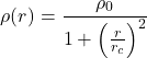
The isothermal model is the cored model, and shown in equation 228,29. It has two parameters: ρ0, which is the central density, or how dense the core of the galaxy is, and rc, the core radius, which is the radius where the density curve stays flat28.
(2) 
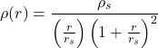
The NFW density profile is shown in equation 321. This model has two parameters which change based on the galaxy: ρs, which is the density scaling parameter and is used to fit the model to the data, and rs, which is where the density of the galaxy changes from ∼1/r to ∼1/r3 in the function21. This is what causes it to be a “cuspy” model, instead of being cored like the isothermal equation.
(3) 
Literature values of NFW halo parameters are often expressed in terms of virial mass, Mvir, and concentration, c. These will be the values we take as parameters in this paper, as they can be converted to the scale density and scale radius for our density curve. The virial radius is given by ![r_{\text{vir}} = \sqrt[3]{ \frac{3 M_{\text{vir}}}{4 \Delta \rho_{\text{crit}}} }](https://nhsjs.com/wp-content/ql-cache/quicklatex.com-df11d1f262159d3a18e22cba5d82980f_l3.png "Rendered by QuickLaTeX.com") , where ρcrit is the critical density of the universe30. Scale radius is given by rs=rvir/c, and the scale density is given by
, where ρcrit is the critical density of the universe30. Scale radius is given by rs=rvir/c, and the scale density is given by ![\rho_s = \frac{M_{\text{vir}}}{4 \pi r_s^3 \left[ \ln(1 + c) - \frac{c}{1 + c} \right]}](https://nhsjs.com/wp-content/ql-cache/quicklatex.com-6d312c6212c6d96fbb669279f9e01187_l3.png "Rendered by QuickLaTeX.com") 9,31.
9,31.
The critical density ρcrit was calculated using  , where the Hubble constant, H0, is set to 67 km/s/Mpc, in order to align with how both this H0 value and the NFW curve itself were calculated using ΛCDM simulations32. The virial overdensity ∆ was set to 200 to match the original NFW study as well as most other rotation curve studies (e.g.,9,30,31).
To convert density to circular velocity, the density function just needs to be converted to a mass function and then plugged into the circular velocity equation. After plugging in each of the density equations for both the isothermal and NFW equations, the simplified solutions come out as equations 4 and 5 respectively.
(4) 
(5) ![\begin{equation*}v_c(r) = \sqrt{ \frac{4 \pi G \rho_s r_s^3}{r} \left[ \ln\left( 1 + \frac{r}{r_s} \right) - \frac{r/r_s}{1 + r/r_s} \right] }\end{equation*}](https://nhsjs.com/wp-content/ql-cache/quicklatex.com-31b93ad49310cf10bd62a131a2b9d7fc_l3.png "Rendered by QuickLaTeX.com")
Source of the Baryonic Velocity Equations
The dark matter models are not the only models necessary to graph the velocity curve; the bulge and disk must also be modeled to create a full velocity profile. For this purpose, we used two widely used profiles: Hernquist for the bulge and Freeman for the disk.
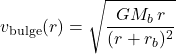
The Hernquist bulge profile is shown in equation 6. This profile comes from the regular circular velocity formula, but it is a specific analytic form of M(r) chosen because it mimics observed bulge light profiles33. This equation has 2 parameters: Mb represents the mass of the entire bulge region, and rb is the scale length, which represents how far out the bulge reaches33.
(6) 
The Freeman disk model is shown in equation 726. This equation has 2 parameters: rd and Σ0. rd represents the disk scale length, or the distance over which the surface brightness of a galaxy’s disk falls by a factor of e. Σ0 represents the central surface mass density of the disk, or the mass per unit area at the disk’s center26. In(x) and Kn(x) are modified Bessel functions of the first and second kind, appearing due to this function modelling a very thin disk, forcing us to compute integrals in cylindrical geometry. The full Bessel functions are given in the appendix.
(7) ![\begin{equation*}v_{\text{disk}}(r) = 4 \pi G \, \Sigma_0 \, r_d \, y^2 \left[ I_0(y) \, K_0(y) - I_1(y) \, K_1(y) \right] , \qquad y \equiv \frac{r}{2 r_d}\end{equation*}](https://nhsjs.com/wp-content/ql-cache/quicklatex.com-60d590b5bad5ef964a2c10794e25270d_l3.png "Rendered by QuickLaTeX.com")
Literature values of parameters for the Freeman disk generally give the disk mass Mb instead of the central density. We use that as the basis for our parameter and convert it to the central density using the equation  when modeling the velocity curve34.
Data Description
We use observation rotation curve data from Zhang & colleagues14, shown in Table 2. This curve was created using a dataset of 13,679 objects in M31 to create the largest collection of velocity measurements for M31 ever. This means it does not only include HI, but uses mixed tracers like stars and halo objects as well14. Some sources of the data include LAMOST DR9, DESI survey, and other relevant publications. The rotation curve stretches out until about 125 kpc, with velocities being split by the authors into disk, bulge, and halo components. Unlike HI-based rotation curves, Zhang 2024 relies on dynamical modeling of multiple tracer populations, introducing additional assumptions in the data14. This is shown by the higher velocity errors in Zhang compared to Carignan 2006, for example35. However, these methods allow access to the outer halo where direct circular velocity measurements are not available. Therefore, while more model-dependent, Zhang 2024 is able to reach much further than traditional HI observations, useful for dark matter models as this is where the M/L ratio should be greatest. Additionally, note that only velocity uncertainties are produced, as radius uncertainties are too small in comparison to significantly impact results.
| Radius (kpc) | Velocity (km/s) | ΔVelocity (km/s) | Radius (kpc) | Velocity (km/s) | ΔVelocity (km/s) |
| 0.22 | 163.24 | 15.61 | 19.38 | 199.73 | 15.19 |
| 0.65 | 210.95 | 18.56 | 8.88 | 233.09 | 32.4 |
| 1.86 | 223.8 | 10.72 | 11.55 | 217.54 | 35.26 |
| 3.19 | 226.79 | 7.96 | 13.55 | 230.53 | 35.63 |
| 4.23 | 213.74 | 8.17 | 15.25 | 212.91 | 36.6 |
| 5.32 | 212.54 | 7.55 | 16.91 | 212.36 | 36.67 |
| 6.27 | 221.94 | 7.2 | 18.68 | 204.64 | 38.1 |
| 7.2 | 223.3 | 8.49 | 20.41 | 220.27 | 37.18 |
| 8.2 | 225.97 | 9.28 | 22.26 | 213.35 | 37.17 |
| 9.14 | 226.63 | 9.07 | 24.12 | 219.28 | 36.73 |
| 9.93 | 223.45 | 10.29 | 26.26 | 217.99 | 35.88 |
| 10.62 | 221.25 | 10.24 | 28.63 | 222.84 | 38.16 |
| 11.25 | 221.17 | 11.16 | 31.23 | 204.28 | 37.89 |
| 11.83 | 213.58 | 9.75 | 34.28 | 210.33 | 38.76 |
| 12.48 | 215.04 | 12.67 | 39.56 | 221.84 | 36.68 |
| 13.37 | 215.12 | 12.82 | 46.21 | 185.33 | 38.68 |
| 14.29 | 217.92 | 13.52 | 52.08 | 182.05 | 38.15 |
| 15.2 | 215.97 | 13 | 54.85 | 196.28 | 38.81 |
| 16.08 | 223.22 | 13.07 | 67.26 | 202.02 | 40.67 |
| 17.21 | 213.32 | 13.44 | 98.74 | 192.59 | 42.23 |
| 18.31 | 213.85 | 15.37 | 123.56 | 168.53 | 41.34 |
Bayesian Analysis
We perform parameter estimation within a Bayesian framework, where the posterior probability distribution of model parameters Θ, given data D, and model M, is determined by Bayes’ theorem
(8) 
Where P(ϴ|D, M) is the posterior, P(D|ϴ, M) is the likelihood, P(ϴ|M) is the prior, and P(D|M) is the evidence (marginal likelihood), and which can be calculated by the following integral:
(9) 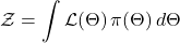
Where  = P(D|M),
  (ϴ) = P(D|ϴ, M), and
  . This integral is usually very challenging to calculate, but that is where dynesty comes in. Dynesty is a python package for estimating both Bayesian posteriors and evidences using the Dynamic Nested Sampling algorithm, making the process far simpler25. All Bayesian analysis in this paper is done using the dynesty package.
For the likelihood function, we assume Gaussian uncertainties in the observed rotation velocities, as is standard practice in astrophysical analyses (e.g.,36,37). The likelihood function is proportional to the following equation:
(10) 
Where Vobs,i is the observed rotation velocity at radius Ri and σi is the observational uncertainty at that point. Note that the constants have been dropped from the usual Gaussian uncertainty equation as nested sampling only necessitates relative likelihoods, so constant normalization factors can be omitted without affecting the results.
Once parameters are finalized, comparing the Isothermal and NFW models using this method is simple. To compare two models M1 and M2, we assume equal prior probabilities for both models, reflecting no prior preference37). This causes the model comparison to reduce to the ratio of Bayesian evidences (Bayes factor):
(11) 
As we are comparing evidences here, we cannot omit the constant in the likelihood functions. This is because depends on the absolute value of (ϴ), making the removal of the constant create a large discrepancy. Therefore, in the likelihood functions that calculate evidence we must include the constant, shown in Equation 13.
(12) 
Additionally, we use the log Bayes factor to compare the fit of our models as it provides superior numerical superiority. In this function, the more positive the value the better model 1 fits, and the more negative the value the better model 2 fits. The log Bayes factor is given as:
(13) 
Priors
The prior ranges used in the Bayesian analysis are listed in Table 2. When creating prior ranges, we decided the spread of the range depending on multiple factors. Rb and Rd have low spreads, as they are based on direct observations17,38,39. Mvir, c, and rc have a slightly wide range due to the methodological variance between studies and, for the first two, a basis in N-body simulations over physical observations9,15,19,21,29,39. Mb, Md, and ρc have a high spread due to not being directly observed and having a high degeneracy with the M/L ratio17,19,21,39,40,41. All priors are based on values from other M31 rotation curve.
| Component | Parameter | Symbol | Range | Units |
| BULGE | Mass | Mb | 3 ×10¹⁰ – 2 ×10¹¹ | M⊙ |
| Scale Length | rb | 4 – 7 | kpc | |
| DISK | Disk Mass | Md | 8 × 10⁹ – 8 × 10¹⁰ | M⊙ |
| Disk Scale Length | rd | 2 – 0.5 | kpc | |
| ISOTHERMAL | Central Density | ρ0 | 10-3 – 10-1 | M⊙ pc-3 |
| Core Radius | rc | 5 – 35 | kpc | |
| NFW | Virial Mass | Mvir | 3 × 10¹¹ – 5 × 10¹² | M⊙ |
| Concentration | c | 10 – 40 | Unitless |
Once parameters are calculated, the median values are reported and used in graphs. The 68%, or 1σ, credible region is reported as asymmetrical errors, corresponding to the 16% and 84% percentiles of the posterior distribution. This is a widely accepted method used for posterior reporting in astrophysics, as it avoids assumptions of Gaussianity and provides proper characterization of potentially skewed posterior distributions (e.g.,21,25,31).
Results
Parameters
In Tables 3 and 4 we report median values for all the parameters, separated by model. The 16% and 84% percentiles of the posterior distribution are provided as asymmetrical errors. Table 3 presents the parameters for the Isothermal model, while Table 4 presents the parameters for the NFW model.
| Component | Parameter | Symbol | median parameter | Units |
| BULGE | Mass | Mb |  | M⊙ |
| Scale Length | rb |  | kpc | |
| DISK | Disk Mass | Md |  | M⊙ |
| Disk Scale Length | rd |  | kpc | |
| ISOTHERMAL | Central Density | ρ0 |  | M⊙ pc-3 |
| Core Radius | rc |  | kpc |
| Component | Parameter | Symbol | median parameter | Units |
| BULGE | Mass | Mb |  | M⊙ |
| Scale Length | rb |  | kpc | |
| DISK | Disk Mass | Md |  | M⊙ |
| Disk Scale Length | rd |  | kpc | |
| NFW | Virial Mass | Mvir |  | M⊙ |
| Concentration | c |  | Unitless |
The posterior distributions for all the parameters values are tight, showcasing that they are very well constrained. The only parameters with significant uncertainties are the central density and core radius, as their uncertainties are large percentages of the median value.
Model Fit
Performing the log Bayes factor test to compare models gives a value of 0.0121 in favor of the isothermal model. This shows essentially no difference between the fits of the models. The prior ranges were shifted by small amounts to check for robustness, but the log bayes factor never exceeded ±2, indicating both models fit about equally well for the M31 data.
Graphs
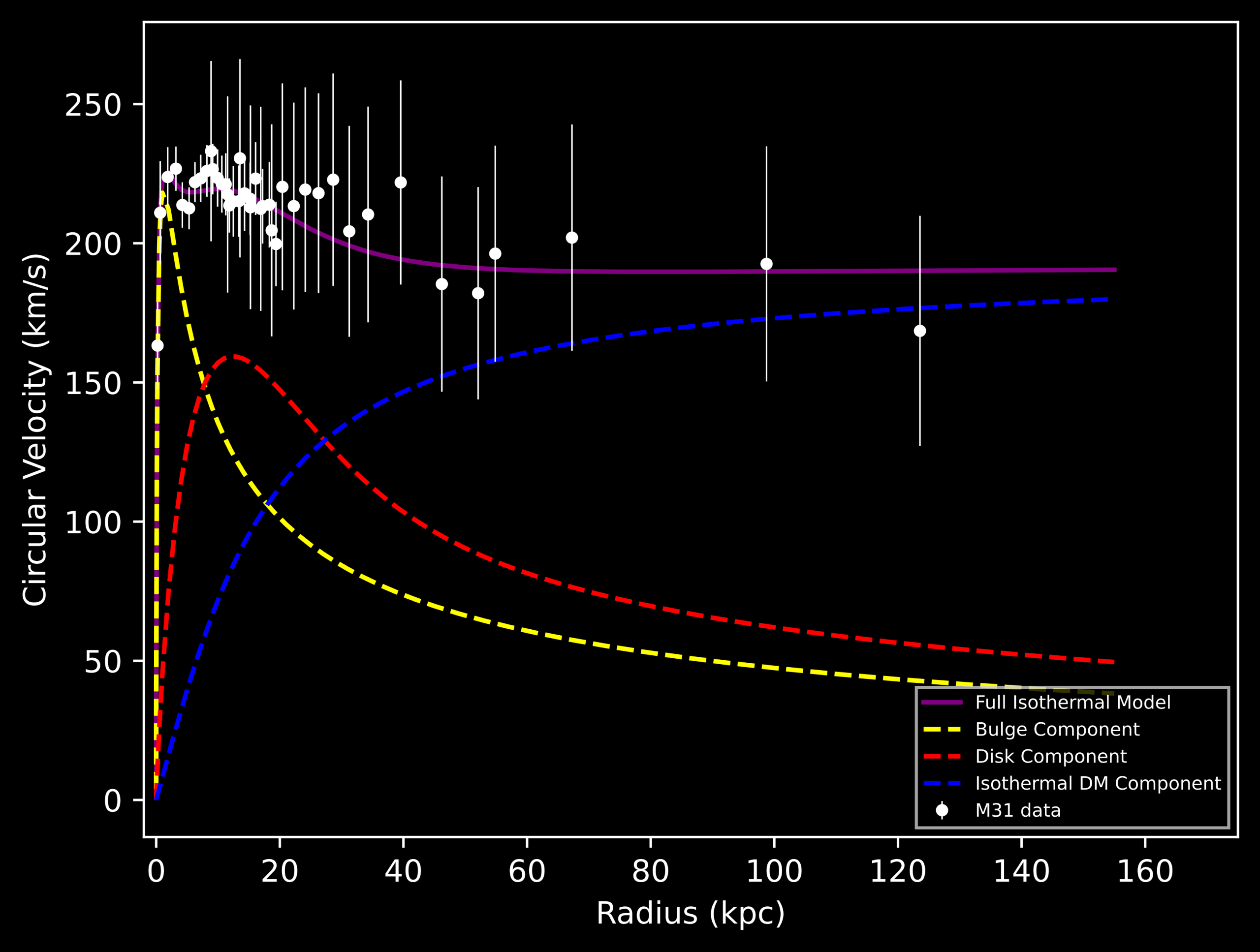
In Figure 1 and Figure 2 we graph the velocity curves of the NFW model and Isothermal model alongside the Zhang 2024 data. Figure 1 graphs the full radius while Figure 2 graphs the inner 60 kpc of the radius.
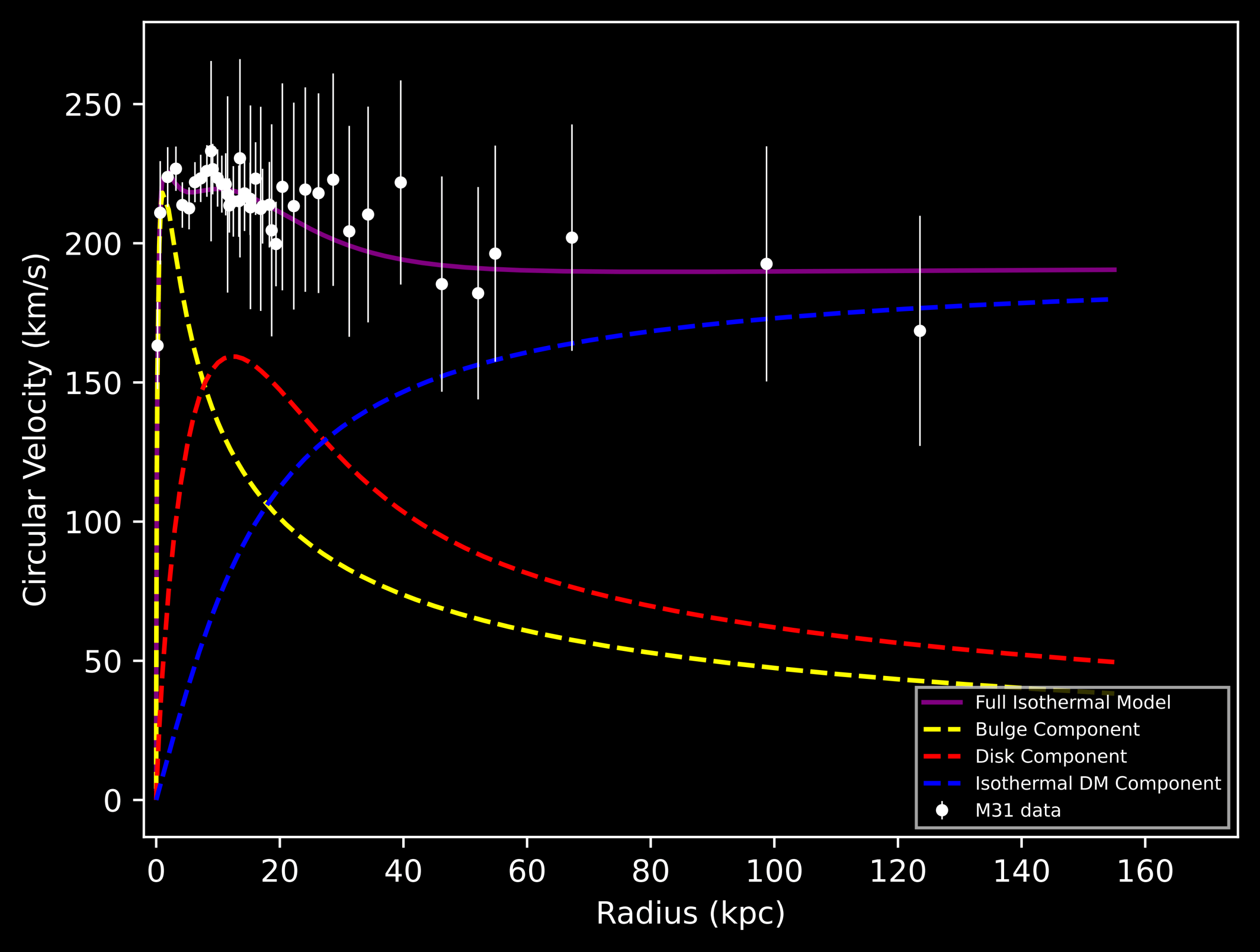
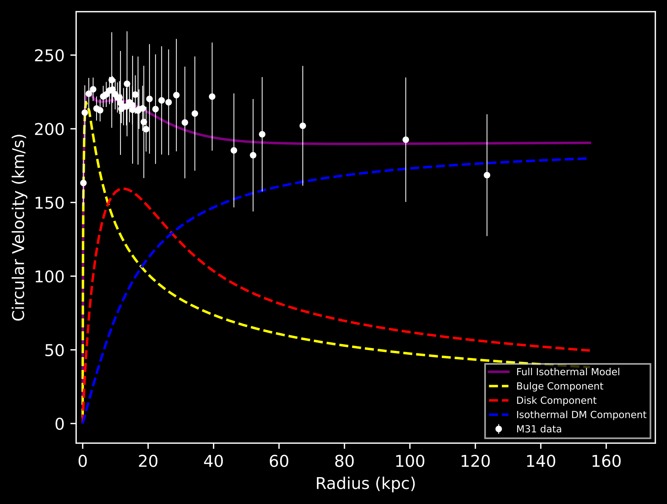
These figures display just how large of an effect parameter degeneracies have on rotation curve models. Both NFW and Isothermal models look almost the same for the first 50 radii until they finally start to diverge. This is the region with the highest bulge and disk percentage, so they are able to overpower any change the models could have due to the dark matter contribution. At larger radii, although there is a divergence, neither model seems to be significantly closer to the data than the other, and the large uncertainties make this more difficult to conclude as well.
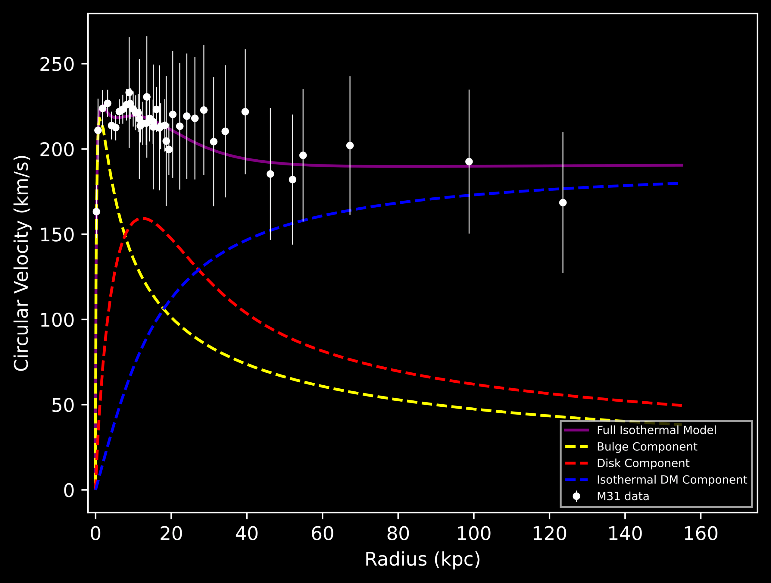
Figure 3 shows the Isothermal model along with all of its split components. Figure 4 the NFW model split into its components as well. These figures showcase how each component contributes to the full velocity curves. The bulge component completely dominates the very low radii, making up almost all the velocity before 1kpc, but then steeply falls off. The NFW component has a much steeper slope at the start, before leveling out very quickly. The isothermal component has a much shallower initial slope but reaches a higher dark matter value later on. It also shows how the disk component is vital for the velocity curve at lower radii. These models also show just how large an effect the degeneracies have on the models. Figure 3 shows the disk components have a very large contribution at lower radii to make up for the isothermal core’s lack of dark matter. In Figure 4, the disk has a far smaller contribution as the cuspy NFW model starts off very dense at lower radii. These showcase how both graphs can be almost equally close to the data at the majority of radii.
Discussion
This paper finds the Isothermal and NFW models to have approximately equal fits on for the M31 data. The log Bayes factor test yielded a result of ~0.01, an almost perfectly equal goodness of fit. Additionally, both graphs stay approximately the same for the first third of radii, the section with the majority of the data points, making any graphical distinction only visible at very large radii.
Both the figures and the data table showcase the flat rotation curves of galaxies. In a galaxy without dark matter, the velocities should have dipped down to around 100km/s, or even lower, just a few kiloparsecs after the peak velocity. Yet, this graph shows the opposite happening, having the graphs stay approximately steady once they reach their maximum velocities.
Cuspy vs Cored
The difference between the cuspy and cored dark matter models are shown very well in Figure 3. The cuspy NFW dark matter component has a much steeper slope at the start, before leveling out very quickly. The Isothermal component has a much shallower initial slope, but reaches a higher and more constant velocity later on in order to compensate. This is exactly how both models are supposed to behave.
Despite differences in the dark matter models themselves, however, both of the full rotation curve models perform approximately the same. This is because of the strong degeneracy between the disk and halo components. When the Isothermal model has a low density at the early radii the disk increases in density to meet the rotation curve data. When the NFW model goes high earlier, the disk stays slow to stay within the data range.
The disk component is only significant at early radii, so at larger radii the models should be more distinct. While both models do diverge at these larger radii, both fit about equally well to the data at large radii. Additionally, the data at large radii was detected from tracers, creating larger scatter and uncertainties at those values. This means if any model is far closer to the data at large radii, it would not cause a statistically meaningful change in its fit due to the large error value.
The negligible difference in Bayesian evidence indicates that neither model provides a significantly more efficient description of the data given the chosen priors. This evidence is based not just on best-fit quality, but on prior volume as well, making this a more significant result. This is not a rare outcome, as much other rotation curve literature is unable to come to specific conclusions on model fit for similar reasons (e.g.,42,37,43).
The low magnitude of the log Bayes factor test points to there being no way to distinguish the Isothermal and NFW models. This is caused by the large number of free parameters, creating strong degeneracies between the components. This allows both models to easily produce flat rotation curves present in the majority of galaxies (e.g.,14,21,37,40). This, combined with the high uncertainty from the data at large uncertainties, makes it difficult to distinguish between the models with the present resources.
Data Analysis
The data analysis for this paper was robust. The use of nested sampling over the traditional MCMC was a big improvement. Nested sampling provided a better model comparison method and handling of the multi-modal posteriors that are common in velocity curve papers. The use of Bayesian statistics more broadly is far more accurate at determining parameter values than frequentist methods in astrophysical contexts.
The use of asymmetric errors provided a more accurate view of the parameters. It is very common for parameters to not have equal likelihoods to increase and decrease from the mid-point of the posterior distributions. Calculating the 68% credible region of these distributions created a more realistic picture of the real possible values of the parameters.
The use of the extended dataset gave an opportunity to compare models at large radii. The models were forced to continue staying flat to model the extended curve, where in other analyses it is possible for the curve to fly both far down or up when looking at the greater radii.
Limitations
Analyzing only a single galaxy means these results only apply to M31. To apply the results more broadly, a larger sample of galaxies would need to be analyzed. Galaxies of varying mass would have needed to be tested to analyze if NFW applies for all cases. This is especially true as core-cusp behavior can be completely different based on the galaxy mass, such as dwarf galaxies showing a more cored density curve.
There are limitations with the model assumptions as well. Our models assume spherical symmetry within the dark matter halo, as well as idealized profiles modeled by each component. Real galaxies have more complex structures that cannot be entirely modeled by these less complex profiles. More complex profiles could have allowed one model a better fit than the other, but it is likely since the differences would have been so minuscule, and that they would have been applied to both models, that the fits would stay approximately equal.
The lack of a gas component is another limitation. Although the gas component makes up a very small fraction of the mass of a galaxy, it does still have an impact. Its inclusion would have been unlikely to change this paper’s conclusions, but it could have changed the specific parameters calculated here, for example.
The uncertainty of the data was a significant limitation. As much of the data, particularly at large radii, came from tracers instead of traditional HI or HII gas, they had much higher uncertainties. This makes it harder to create models around the data points, as they are less likely to exactly fit the data. Higher quality data could allow a more concrete fit for both models.
One more uncertainty is prior range choice. Nested sampling relies on prior choice in a large way to calculate model accuracy. Deciding priors is a subjective decision and could therefore alter the outcomes of model comparison. This paper attempted to choose priors based on previous bodies of work, and calculated the Bayes factor with different prior choices, but it is possible better ranges could have been chosen which could have changed results in one model’s favor.
This investigation did not look at other dark matter profiles. Other popular density profiles such as Einasto and Burkert may have provided even better fits, but were not discussed here. It is possible one of these models has better fits than the NFW and Isothermal models, which would have changed the conclusions of this paper.
Future studies may look at restricting the stellar components of the models, such as by utilizing independent mass tracers to constrain the mass. This would allow for degeneracies to be reduced, creating more conclusive models.
Conclusion
This study compared the Navarro-Frenk-White and Isothermal dark matter density models to simulate the observed velocity curve of M31. Robust parameter calculations were produced using a nested sampling approach for each individual model. Log Bayes factor analysis produced a value close to 0, showing no real preference between the models. These conclusions show the systematic problems with measuring velocity curves with high degeneracies. These conclusions are specifically applicable to M31, though similar methods will be applicable for all galaxies. Higher quality data and more restrictions on the stellar mass are needed to form more specific conclusions about these dark matter models.
Acknowledgements
I would like to thank Imran Sultan and Tjitske Starkenburg from CIERA for taking time to read through and critique earlier drafts of my research, despite not being my formal advisors. Their advice gave me much needed direction for how to refine and expand my research.
References
- Rubin, V. C., Ford, W. K., and Thonnard, N., “Rotational properties of 21 SC galaxies with a large range of luminosities and radii, from NGC 4605 (R=4kpc) to UGC 2885 (R=122kpc).”, The Astrophysical Journal, vol. 238, IOP, pp. 471–487, 1980. doi.org/10.1086/158003. [↩] [↩]
- Bosma, A., “21-cm line studies of spiral galaxies. II. The distribution and kinematics of neutral hydrogen in spiral galaxies of various morphological types.”, The Astronomical Journal, vol. 86, IOP, pp. 1825–1846, 1981. doi.org/10.1086/113063. [↩]
- Sofue, Y. and Rubin, V., “Rotation Curves of Spiral Galaxies”, Annual Review of Astronomy and Astrophysics, vol. 39, pp. 137–174, 2001. doi.org/10.1146/annurev.astro.39.1.137. [↩]
- de Blok, W. J. G., McGaugh, S. S., and Rubin, V. C., “High-Resolution Rotation Curves of Low Surface Brightness Galaxies. II. Mass Models”, The Astronomical Journal, vol. 122, no. 5, IOP, pp. 2396–2427, 2001. doi.org/10.1086/323450. [↩] [↩] [↩] [↩] [↩] [↩]
- Bullock, J. S. and Boylan-Kolchin, M., “Small-Scale Challenges to the ΛCDM Paradigm”, Annual Review of Astronomy and Astrophysics, vol. 55, no. 1, pp. 343–387, 2017. doi.org/10.1146/annurev-astro-091916-055313. [↩]
- Marchesini, D., D’Onghia, E., Chincarini, G., Firmani, C., Conconi, P., Molinari, E., and Zacchei, A., “Hα Rotation Curves: The Soft Core Question”, Astrophys. J. vol 575, no. 2, pp. 801–813, 2002. doi.org/10.1086/341475. [↩]
- de Blok, W. J. G., The Core-Cusp Problem, Advances in Astronomy, 14 pages, 2010. https://doi.org/10.1155/2010/789293. [↩]
- Dubinski, J. and Carlberg, R. G., “The Structure of Cold Dark Matter Halos”, The Astrophysical Journal, vol. 378, IOP, p. 496, 1991. doi.org/10.1086/170451. [↩]
- Navarro, J. F., Frenk, C. S., and White, S. D. M., “The Structure of Cold Dark Matter Halos”, The Astrophysical Journal, vol. 462, IOP, p. 563, 1996. doi.org/10.1086/177173. [↩] [↩] [↩] [↩] [↩]
- Gentile, G., Salucci, P., Klein, U., Vergani, D., and Kalberla, P., “The cored distribution of dark matter in spiral galaxies”, Monthly Notices of the Royal Astronomical Society, vol. 351, no. 3, OUP, pp. 903–922, 2004. doi.org/10.1111/j.1365-2966.2004.07836.x. [↩]
- Kent, S. M., “Dark matter in spiral galaxies. I. Galaxies with optical rotation curves.”, The Astronomical Journal, vol. 91, IOP, pp. 1301–1327, 1986. doi.org/10.1086/114106. [↩]
- Maria C Straight, Michael Boylan-Kolchin, James S Bullock, Philip F Hopkins, Xuejian Shen, Lina Necib, Alexandres Lazar, Andrew S Graus, Jenna Samuel, Central densities of dark matter haloes in fire-2 simulations of low-mass galaxies with cold dark matter and self-interacting dark matter, Monthly Notices of the Royal Astronomical Society, Volume 543, Issue 3, November 2025, Pages 1995–2005, https://doi.org/10.1093/mnras/staf1539 [↩]
- Di Cintio, A., “The dependence of dark matter profiles on the stellar-to-halo mass ratio: a prediction for cusps versus cores”, Monthly Notices of the Royal Astronomical Society, vol. 437, no. 1, OUP, pp. 415–423, 2014. doi.org/10.1093/mnras/stt1891. [↩] [↩]
- Xiangwei Zhang, Bingqiu Chen, Pinjian Chen, Jiarui Sun, Zhijia Tian, The rotation curve and mass distribution of M31, Monthly Notices of the Royal Astronomical Society, Volume 528, Issue 2, February 2024, Pages 2653–2666, https://doi.org/10.1093/mnras/stae025 [↩] [↩] [↩] [↩] [↩] [↩] [↩] [↩]
- Hammer, F., “Dark matter fraction derived from the M31 rotation curve”, Astronomy and Astrophysics, vol. 694, Art. no. A16, EDP, 2025. doi.org/10.1051/0004-6361/202452753. [↩] [↩] [↩]
- Law, B.M. Comparison of a new type of Dark Matter with the Milky Way and M31 grand rotation curves. Sci Rep 14, 24090, 2024. https://doi.org/10.1038/s41598-024-74884-6. [↩]
- Baker, T., Psaltis, D., and Skordis, C., “Linking Tests of Gravity on All Scales: from the Strong-field Regime to Cosmology”, The Astrophysical Journal, vol. 802, no. 1, Art. no. 63, IOP, 2015. doi.org/10.1088/0004-637X/802/1/63. [↩] [↩] [↩]
- Bariego-Quintana, A., Llanes-Estrada, F. J., “No evidence for Keplerian taper of far-out galactic rotation in the SPARC galaxy database”, New Astronomy, vol. 126, 102537, 2026, https://doi.org/10.1016/j.newast.2026.102537. [↩] [↩]
- Banerjee, A. and Jog, C. J., “The Flattened Dark Matter Halo of M31 as Deduced from the Observed H I Scale Heights”, The Astrophysical Journal, vol. 685, no. 1, IOP, pp. 254–260, 2008. doi.org/10.1086/591223. [↩] [↩] [↩]
- J. J. Geehan, M. A. Fardal, A. Babul, P. Guhathakurta, Investigating the Andromeda stream — I. Simple analytic bulge—disc—halo model for M31, Monthly Notices of the Royal Astronomical Society, Volume 366, Issue 3, March 2006, Pages 996–1011, https://doi.org/10.1111/j.1365-2966.2005.09863.x [↩]
- Tempel, E., Tamm, A., and Tenjes, P., “Visible and dark matter in M 31 – II. A dynamical model and dark matter density distribution”, arXiv e-prints, Art. no. arXiv:0707.4374, 2007. doi.org/10.48550/arXiv.0707.4374. [↩] [↩] [↩] [↩] [↩] [↩] [↩] [↩]
- Lelli, F. Gas dynamics in dwarf galaxies as testbeds for dark matter and galaxy evolution. Nat Astron 6, 35–47, 2022. https://doi.org/10.1038/s41550-021-01562-2 [↩]
- Kumar, D., Rani, N., Jain, D., Mahajan, S., and Mukherjee, A., “Study of Various Dark Matter Halo Profiles in Milky Way and M31 Galaxies within the Standard Cosmology Framework”, Research in Astronomy and Astrophysics, vol. 25, no. 7, Art. no. 075005, IOP, 2025. doi.org/10.1088/1674-4527/addc1b. [↩] [↩]
- Katz, H., Lelli, F., McGaugh, S. S., Di Cintio, A., Brook, C. B., and Schombert, J. M., “Testing feedback-modified dark matter haloes with galaxy rotation curves: estimation of halo parameters and consistency with ΛCDM scaling relations”, Monthly Notices of the Royal Astronomical Society, vol. 466, no. 2, OUP, pp. 1648–1668, 2017. doi.org/10.1093/mnras/stw3101. [↩]
- Joshua S Speagle, dynesty: a dynamic nested sampling package for estimating Bayesian posteriors and evidences, Monthly Notices of the Royal Astronomical Society, Volume 493, Issue 3, April 2020, Pages 3132–3158, https://doi.org/10.1093/mnras/staa278 [↩] [↩] [↩]
- Courteau, S., “Galaxy masses”, Reviews of Modern Physics, vol. 86, no. 1, APS, pp. 47–119, 2014. doi.org/10.1103/RevModPhys.86.47. [↩] [↩] [↩] [↩] [↩]
- Pavel E Mancera Piña, Filippo Fraternali, Tom Oosterloo, Elizabeth A K Adams, Enrico di Teodoro, Cecilia Bacchini, Giuliano Iorio, The impact of gas disc flaring on rotation curve decomposition and revisiting baryonic and dark matter relations for nearby galaxies, Monthly Notices of the Royal Astronomical Society, Volume 514, Issue 3, August 2022, Pages 3329–3348, https://doi.org/10.1093/mnras/stac1508 [↩] [↩]
- Gunn, J. E. and Gott, J. R., “On the Infall of Matter Into Clusters of Galaxies and Some Effects on Their Evolution”, The Astrophysical Journal, vol. 176, IOP, p. 1, 1972. doi.org/10.1086/151605. [↩] [↩]
- de Blok, W. J. G., Walter, F., Brinks, E., Trachternach, C., Oh, S.-H., and Kennicutt, R. C., “High-Resolution Rotation Curves and Galaxy Mass Models from THINGS”, The Astronomical Journal, vol. 136, no. 6, IOP, pp. 2648–2719, 2008. doi.org/10.1088/0004-6256/136/6/2648/ [↩] [↩]
- Bryan, G. L. and Norman, M. L., “Statistical Properties of X-Ray Clusters: Analytic and Numerical Comparisons”, The Astrophysical Journal, vol. 495, no. 1, IOP, pp. 80–99, 1998. doi.org/10.1086/305262. [↩] [↩]
- Klypin, A., Zhao, H., and Somerville, R. S., “ΛCDM-based Models for the Milky Way and M31. I. Dynamical Models”, The Astrophysical Journal, vol. 573, no. 2, IOP, pp. 597–613, 2002. doi.org/10.1086/340656. [↩] [↩] [↩]
- Planck Collaboration, “Planck 2018 results. VI. Cosmological parameters”, Astronomy and Astrophysics, vol. 641, Art. no. A6, EDP, 2020. doi.org/10.1051/0004-6361/201833910. [↩]
- Hernquist, L., “An Analytical Model for Spherical Galaxies and Bulges”, The Astrophysical Journal, vol. 356, IOP, p. 359, 1990. doi.org/10.1086/168845. [↩] [↩]
- Hakobyan, A. A., Mamon, G. A., Petrosian, A. R., Kunth, D., and Turatto, M., “The radial distribution of core-collapse supernovae in spiral host galaxies”, Astronomy and Astrophysics, vol. 508, no. 3, EDP, pp. 1259–1268, 2009. doi.org/10.1051/0004-6361/200912795. [↩]
- Carignan, C., Chemin, L., Huchtmeier, W. K., and Lockman, F. J., “The Extended H I Rotation Curve and Mass Distribution of M31”, The Astrophysical Journal, vol. 641, no. 2, IOP, pp. L109–L112, 2006. doi.org/10.1086/503869. [↩]
- Roman-Oliveira, F., Rizzo, F., and Fraternali, F., “Dynamical modelling and the origin of gas turbulence in z ∼ 4.5 galaxies”, Astronomy and Astrophysics, vol. 687, Art. no. A35, EDP, 2024. doi.org/10.1051/0004-6361/202348828. [↩]
- Hassan, D.S., Danarianto, M.D. & Sulaksono, A. “The Milky Way and M31 rotation curves in Yukawa gravity: phenomenology and Bayesian analysis”, Eur. Phys. J. C 86, 198, 2026. https://doi.org/10.1140/epjc/s10052-026-15428-2 [↩] [↩] [↩] [↩]
- Corbelli, E., Lorenzoni, S., Walterbos, R., Braun, R., and Thilker, D., “A wide-field H I mosaic of Messier 31. II. The disk warp, rotation, and the dark matter halo”, Astronomy and Astrophysics, vol. 511, Art. no. A89, EDP, 2010. doi.org/10.1051/0004-6361/200913297. [↩]
- Chemin, L., Carignan, C., and Foster, T., “H I Kinematics and Dynamics of Messier 31”, The Astrophysical Journal, vol. 705, no. 2, IOP, pp. 1395–1415, 2009. doi.org/10.1088/0004-637X/705/2/1395. [↩] [↩] [↩]
- Aniyan, S., “Resolving the Disk-Halo Degeneracy: A look at M74”, in Formation and Evolution of Galaxy Outskirts, 2017, vol. 321, pp. 267–267. doi.org/10.1017/S1743921316008814. [↩] [↩]
- Tamm, A., Tempel, E., Tenjes, P., Tihhonova, O., and Tuvikene, T., “Stellar mass map and dark matter distribution in M 31”, Astronomy and Astrophysics, vol. 546, Art. no. A4, EDP, 2012. doi.org/10.1051/0004-6361/201220065 [↩]
- Hammer, F., “Dark matter fraction derived from the M31 rotation curves”, Astronomy and Astrophysics, vol. 694, Art. no. A16, EDP, 2025. doi.org/10.1051/0004-6361/202452753. [↩]
- McGaugh, S. S., “The Baryonic Mass─Halo Mass Relation of Extragalactic Systems”, The Astrophysical Journal, vol. 1001, no. 1, Art. no. 65, IOP, 2026. doi.org/10.3847/1538-4357/ae4ecc. [↩]