Abstract
Microplastics are a global environmental concern with widespread impacts on marine ecosystems. Predicting oceanic microplastic concentration remains underexplored, as most machine-learning approaches focus on regional settings and rely on features not consistently available worldwide. We propose a global framework that uses universally available spatial inputs (latitude, longitude, ocean, month) augmented with 256-dimensional satellite-derived geo-embeddings. Using ~ 20,000 observations from the NOAA NCEI Marine Microplastics Database, we evaluate this framework using class weighted training with Support Vector Classifier (SVC), Random Forest (RF), and Gradient Boosting (GB) models. Under stratified cross-validation, ensemble models outperform SVC, while geo-embeddings produce consistent improvements across both RF and GB models. At the ocean level, improvements are strongest in class-balanced regions such as the Pacific, where embeddings improve both Macro-F1 (8.5 %) and Weighted-F1 (10 %), indicating better minority class recognition. Gains are more modest or inconsistent in imbalanced or data-sparse regions. Aggregated globally, embeddings improve performance primarily in Weighted-F1 (5-8 %), while Macro-F1 gains remain limited. An ablation using Radial Basis Function (RBF) features suggests that geo-embeddings capture richer spatial context beyond coordinate transformations. Leave-one-ocean-out evaluation reveals sensitivity to spatial distribution shift, particularly due to differences in class distributions between training and test domains. In this setting, embeddings improve performance in regions such as the Atlantic and Arctic but degrade performance in label-diverse domains such as the Pacific. Notably, embeddings consistently improve performance for the majority class across oceans. Overall, pre-trained geo-embeddings improve in-domain performance under standard evaluation but generalize inconsistently under spatial distribution shift, motivating more robust spatial modeling and domain adaptation approaches for global marine monitoring.
Introduction
Plastic pollution has become a major environmental issue in the 21st century. Over time, plastic waste breaks down into microplastics (<5 mm), which are now widespread in the oceans. According to the National Oceanic and Atmospheric Administration, these particles are extremely difficult to trace, yet they pose a global risk: marine organisms ingest them, and they can eventually reach humans through seafood consumption. As most plastic waste ultimately ends up in the ocean, microplastic contamination has become a planetary-scale challenge. Global observational and modeling studies further confirm the scale and complexity of the problem by showing that plastics accumulate at large scales1,2,3 and are transported across oceans.
Prior work on microplastic prediction and environmental modeling spans three main areas: oceanographic transport models, localized and data-driven machine learning approaches, and recent advances in geospatial representation learning and foundation models for Earth observation.
Oceanographic Transport Models
Transport-based approaches model the movement and accumulation of plastic debris using Lagrangian particle tracking4 parametric equations5 and ocean circulation models6. These models provide global insights into debris pathways and large-scale accumulation zones but depend on detailed physical inputs that are difficult to obtain and validate consistently at a global scale.
Localized Machine Learning Approaches
Machine learning (ML) has been applied to microplastic research in several ways. Some studies focus on classifying microplastic types in the laboratory, for example using ML on spectroscopic FTIR data7,8,9. Other studies predict concentrations in specific regions with specialized features, such as mussel size and substrate type in the Western Black Sea10, or pH and salinity in Vietnamese peatlands11. While powerful these approaches remain localized and cannot generalize on a global scale due to their reliance on features that are not available globally. Recently, machine learning models have been developed for freshwater systems at a global scale12,13. However, these rely on land-based predictors like cropland, urban cover, runoff, and population density; features that are not meaningful or consistently available in marine environments.
A separate line of research focuses on detecting plastic debris using imaging and remote sensing. Satellite and imaging-based approaches can identify visible macro plastics and characterize debris distributions14. However, these methods are limited to locations where measurements or imagery are available and do not provide global predictions of microplastic concentration levels in the oceans.
Geospatial Representation Learning And Foundation Models
Beyond microplastic-specific studies, ML has been widely used for environmental prediction tasks. Models such as Random Forests are commonly applied due to their ability to capture nonlinear relationships in heterogeneous environmental data15. ML methods more broadly have shown effectiveness in modeling complex Earth system processes16. However, spatial prediction introduces additional challenges: standard validation approaches can lead to overly optimistic estimates when spatially correlated samples appear in both training and test sets17, making generalization to unseen regions difficult.
Recent advances in geospatial representation learning provide an alternative to manually engineered features. Prior work has shown that spatial context can be learned directly from data, for example through representations derived from satellite imagery18,19. Additional work in remote sensing and large-scale geospatial learning demonstrates the ability to encode transferable representations of geographic locations from globally available data20. Recent approaches such as SatCLIP extend this idea by learning global location embeddings from satellite imagery21. Emerging work on large-scale Earth observation foundation models further shows that geo-spatial representations can support high fidelity prediction of downstream environmental tasks such as land cover classification22 and air quality, ocean waves, tropical and cyclone tracks23.
Existing approaches do not enable global prediction of microplastic concentration levels, as they are restricted to spatially local observations or rely on specialized features that are not consistently available across regions, limiting their applicability and generalization to unsampled areas. More broadly, these approaches fall into two categories: localized machine learning models that depend on region-specific environmental features, and transport-based models that require detailed physical inputs and assumptions. Localized models achieve strong performance within limited regions but lack transferability, while transport models provide global coverage but are difficult to scale consistently and validate across regions. As a result, both approaches fail to support planetary-scale prediction: localized models cannot generalize beyond regions with available features, while transport models depend on inputs that are difficult to obtain and validate globally. This creates a gap for methods that can leverage globally available inputs such as transferable spatial representations learned from large-scale geospatial data. Building on recent advances in geospatial representation learning, our approach leverages such representations to enable prediction of microplastic concentration levels across oceans globally without reliance on localized environmental features.
We apply globally transferable spatial representations by incorporating geo-embeddings derived from satellite data using SatCLIP. Prediction of microplastic concentration levels is thus framed as a global spatial modeling problem rather than a locally engineered feature problem. We develop a machine-learning framework for predicting ocean microplastic concentrations using the NOAA NCEI Marine Microplastics Database24, which categorizes concentrations into five levels: Very Low, Low, Medium, High, and Very High—enabling prediction of actionable categories relevant for environmental monitoring and policy. This paper makes three key contributions: (1) a prediction framework that leverages globally available spatial inputs instead of region-specific environmental features; (2) the application of geo-embeddings to capture spatial context and enable prediction across all oceans, including under-sampled regions; and (3) a planetary-scale evaluation using multiple machine-learning models. Given strong imbalance across both labels and oceans, performance is evaluated using Macro-F1 and Weighted-F1, which better reflect minority-class recognition than overall accuracy. Among the models tested—Support Vector Classifiers25, Random Forests26 and Gradient Boosting27, ensemble models consistently outperform SVC, while geo-embeddings produce consistent improvements across both RF and GB models in a stratified cross validation setting. However, the effectiveness of these pre-trained geo-embeddings varies across oceans and under spatial distribution shift, motivating further study of domain adaptation and transferable spatial modeling approaches.
Methods
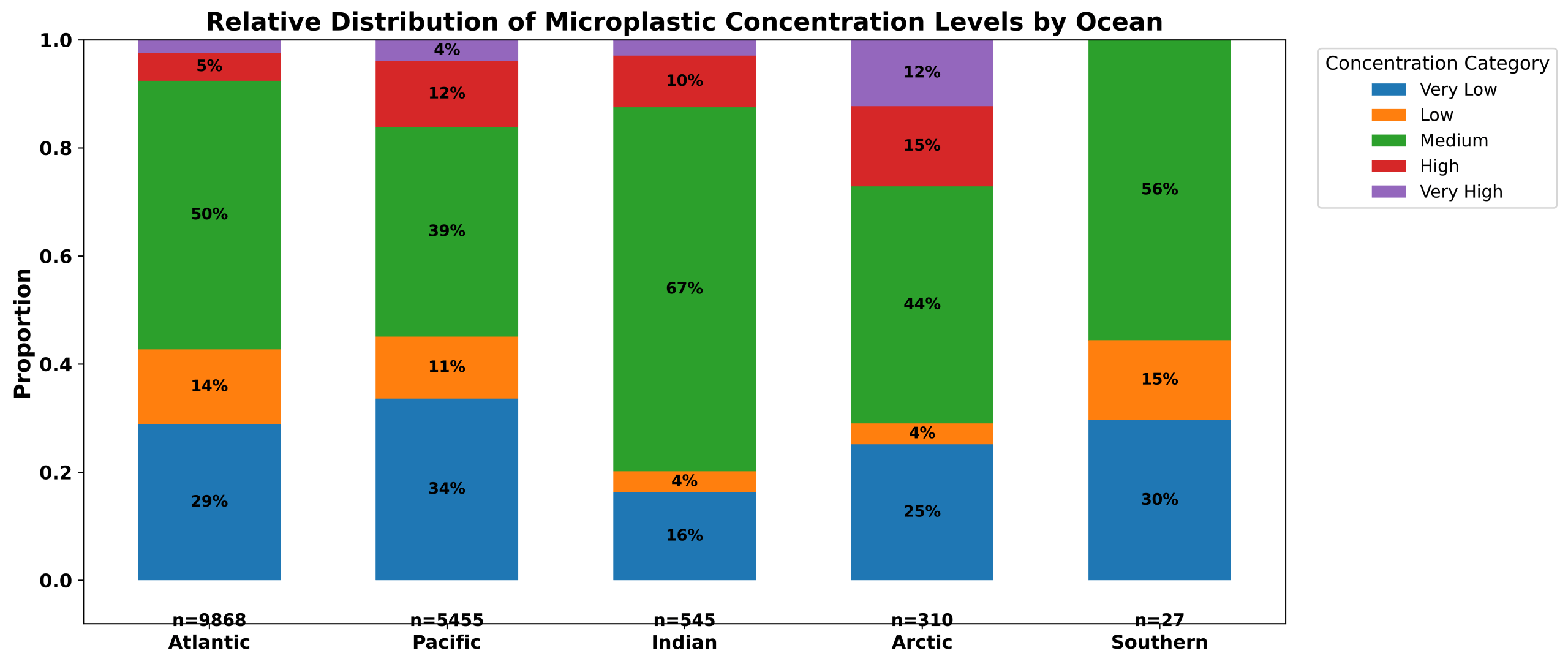
We use the NOAA NCEI Marine Microplastics Database, a public dataset comprising approximately 20,000 measurements from locations worldwide across all major oceans. Each record includes geographic and sampling information (latitude, longitude, depth, and date) along with the measured concentration of microplastic and categorical concentration labels (Very Low, Low, Medium, High, Very High) provided directly by the NOAA dataset. The dataset is imbalanced in two ways. First, the distribution of labels is skewed, with Medium as the majority class across all oceans as shown in Figure 1. Second, the number of observations differs greatly by ocean: the Atlantic and Pacific Oceans dominate the dataset with 9868 and 5455 observations, respectively, while the Indian, Arctic, and especially Southern Oceans are sparsely represented with 545, 310 and 27 observations, respectively. Class imbalance is addressed by using inverse class weighting during training, such that all classes are given equal weight during model training. In addition, we evaluate model performance separately for each ocean to assess regional generalization under uneven sampling. We compare three machine learning classifiers: Support Vector Classifier (SVC), Random Forest (RF), and Gradient Boosting (GB). RF and GB are ensemble methods that combine multiple decision trees to capture non-linear patterns and improve robustness. SVC serves as a baseline classifier for comparison with ensemble methods.
Model performance is evaluated using the F1 score, which balances precision (correctness of positive predictions) and recall (coverage of actual positives). An F1 of 1.0 indicates perfect performance, while 0 indicates no predictive performance. We report Macro-F1, which gives equal weight to all classes and Weighted-F1, which averages class-specific F1 scores using class frequencies (reflecting performance on imbalanced data). Accuracy alone is misleading in this setting because it can appear high by simply predicting the majority class in heavily represented oceans. We therefore evaluate performance under both standard cross-validation and leave-one-ocean-out cross-validation (LOOCV) settings to assess generalization under class and regional imbalance.
In all models, we use baseline spatial inputs consisting of latitude, longitude, and one-hot encoded representations of month and ocean identity that are already present in the dataset. We further augment these features using geo-embeddings derived from SatCLIP, a foundational AI model trained on global satellite imagery. While latitude and longitude identify a location geometrically, geo-embeddings provide a high-dimensional representation of the surrounding geographic context. These embeddings capture large-scale environmental patterns, such as land–water distribution and surface characteristics, enabling the model to recognize similarities between distant locations with comparable environmental conditions. By incorporating this richer spatial representation, our framework supports improved predictive performance across diverse geographic regions while enabling evaluation in under-sampled oceans such as the Arctic and Southern Oceans without relying on specially engineered environmental features.
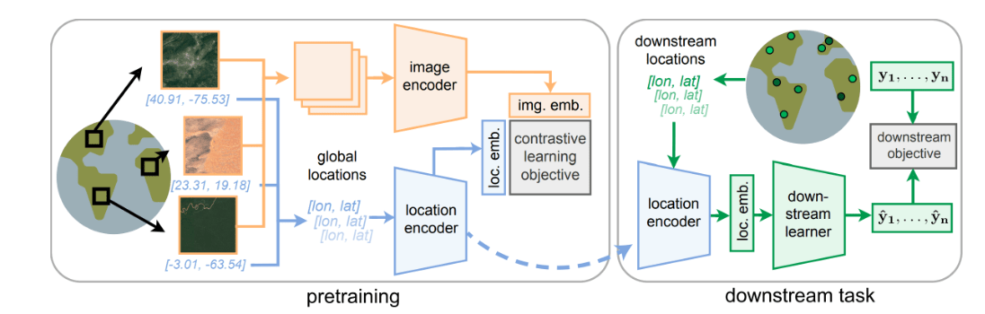
The SatCLIP modeling framework pre-trains an image encoder and a location encoder, as shown in Figure 2. The location encoder fc: (x, y) → Rd takes in 2-dimensional coordinates (x, y) and returns a d-dimensional embedding. The image encoder fi : Rmxnxk → Rd takes in an image I ∈ Rmxnxk and also returns a d-dimensional embedding. In this study we use the pretrained location encoder fc in a frozen form for the downstream task of predicting microplastic concentration levels. The location encoder produces d-dimensional embeddings (d = 256). These embeddings are concatenated with baseline spatial inputs and used as additional numerical predictors.
Experimental Design
We designed experiments to evaluate the ability of universally available spatial inputs and geo-embeddings to support prediction of microplastic concentration levels under both standard and cross-ocean evaluation settings. For each model, we trained two variants:
- Baseline – using only latitude, longitude, ocean, and month. We include month as a coarse temporal feature to capture potential time-dependent variation in observations. To isolate the contribution of temporal information, we perform an ablation study on the Gradient Boosting (GB) model, comparing performance with and without the month feature.
- Baseline + Embeddings – using the same features plus geo-embeddings. These embeddings are generated by SatCLIP’s pre-trained location encoder using latitude and longitude inputs, as illustrated in the downstream task block in Figure 2. For models sensitive to feature scale (e.g., SVC), we apply z-score standardization (zero mean, unit variance) to the geo-embeddings before concatenating with the baseline features. Tree-based models (RF, GB) are trained on unscaled features.
All models were trained using the scikit-learn Python library28. The Support Vector Classifier (SVC) uses a Radial Basis Function (RBF) kernel, with hyperparameters tuned using GridSearchCV over the regularization parameter C∈{0.1,1,10,100} and kernel width γ∈{“scale”, “auto”, 10⁻³, 10⁻², 10⁻¹}. Random Forest (RF) hyperparameters are tuned using GridSearchCV over number of estimators n∈{100,200,300}, minimum number of samples per leaf m∈{1,5,10,15} and max depth d∈{10,12,14}. Gradient Boosting (GB) hyperparameter value ranges for n and m are the same as RF while the max depth d∈{2,3,4}. Hyperparameter tuning is performed independently for each baseline and embedding-augmented model variant using the same search space, cross-validation protocol, and scoring metric to ensure fair comparison across feature settings. Model selection is performed using cross-validation with Macro-F1 as the scoring metric. Final selected hyperparameters for all models are provided in Appendix A.
We used 5-fold stratified cross-validation (StratifiedKFold, k = 5) to obtain robust performance estimates while preserving class proportions across folds. In addition to stratified cross-validation, we evaluate generalization under spatial distribution shift using a leave-one-ocean-out cross-validation (LOOCV) protocol. In this setting, all samples from one ocean are held out as the test set while models are trained on the remaining oceans. This process is repeated for each ocean, enabling evaluation of model transferability to un-seen geographic regions with differing class distributions and sampling densities.
We evaluated models using Macro-F1 and Weighted-F1 scores. Macro-F1 treats each class equally, while Weighted-F1 reflects overall performance when classes are imbalanced. We examined how these metrics varied across oceans as well as globally. By comparing baseline and embedding variants side by side, we directly measured the contribution of geo-embeddings to predicting marine microplastic levels.
Results
Model Performance Across Oceans
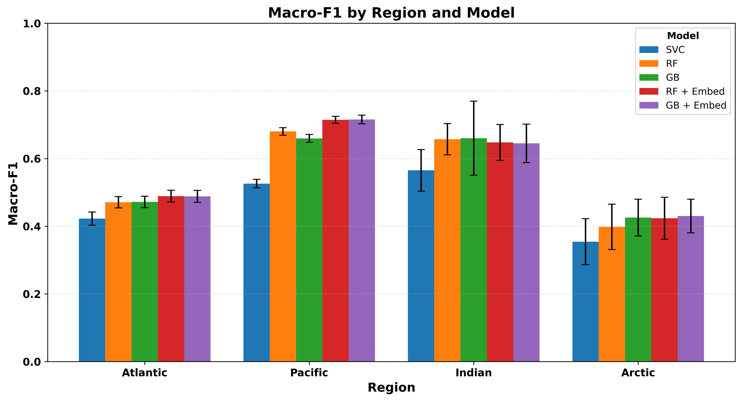
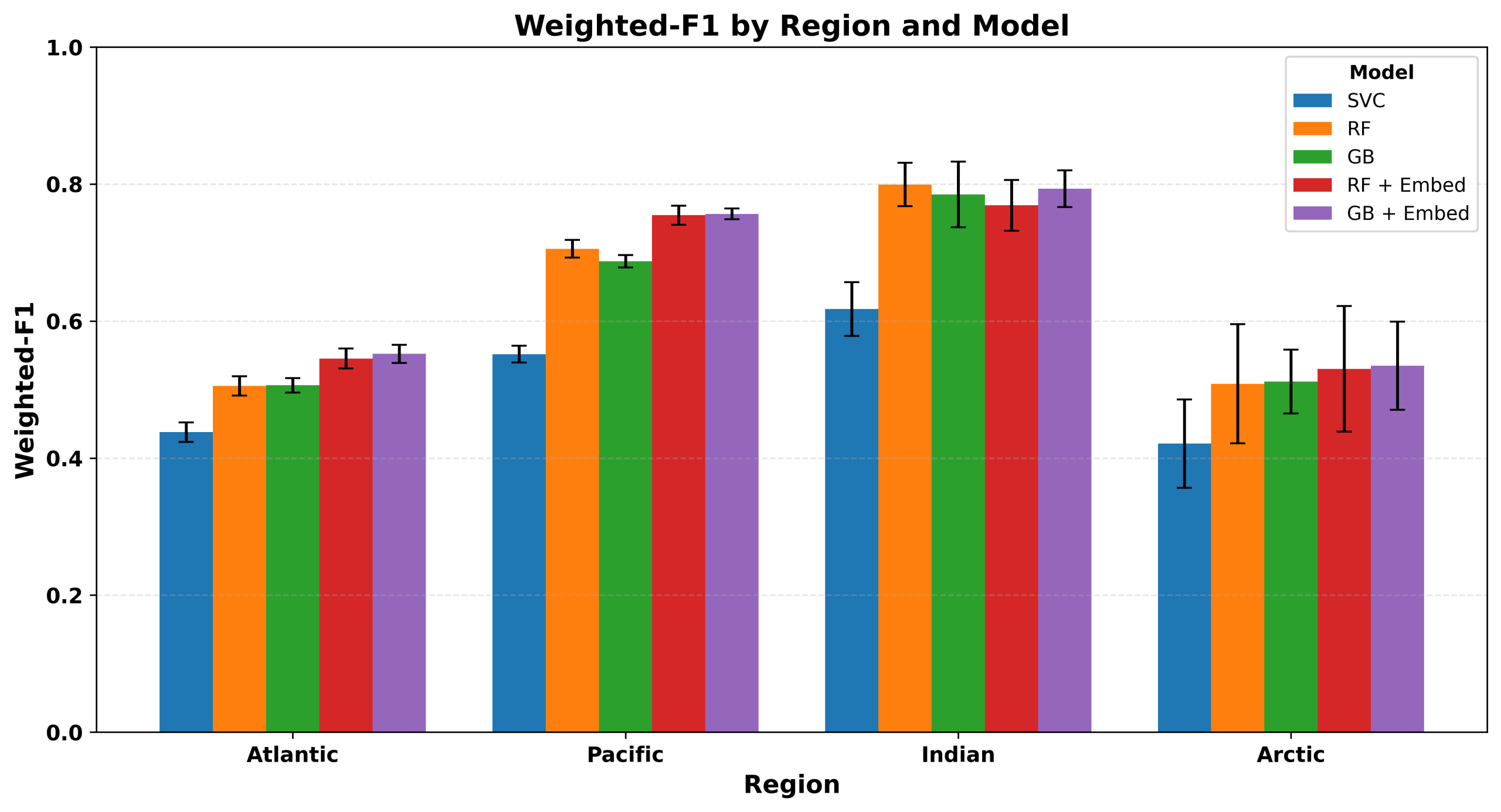
We evaluate model performance across oceans to assess generalization under varying data availability and label distributions. Figures 3 and 4 compare baseline models with their embedding-augmented counterparts using Macro-F1 and Weighted-F1. Ensemble models such as RF and GB consistently outperform SVC across all oceans, indicating the importance of higher-capacity nonlinear models for the task of predicting microplastic concentration levels. The following analysis therefore focuses on the effects of geo-embeddings in the RF and GB models. Performance in the Southern Ocean is excluded from analysis due to its extremely small sample size (≈ 27 total samples, ≈ 5 per fold), which leads to high variance and unreliable estimates. Per-class precision, recall, and F1-scores for the GB baseline and embedding-augmented models are provided in Appendix B. Per-fold model performance for each of the models is shown in Appendix C.
Effect of Embeddings
Embeddings provide the largest improvements in high-support regions, particularly the Pacific and Atlantic Oceans. For GB, Macro-F1 improves by about 8.5% (p-value ≈ 0.03) in the Pacific and about 3.5 % in the Atlantic. Weighted-F1 shows larger gains, of about 10% (p-value ≈ 0.03) in the Pacific and around 9% (p-value ≈ 0.03) in the Atlantic. For RF, a similar pattern is observed, with Macro-F1 increasing by approximately 5% (p-value ≈ 0.03) in the Pacific and 3.9 % in the Atlantic, and Weighted-F1 improving by roughly 7 % (p-value ≈ 0.03) in the Pacific and around 8% (p-value ≈ 0.03) in the Atlantic. These improvements are statistically significant in the Pacific for both Macro-F1 and Weighted-F1, and in the Atlantic for Weighted-F1, while Macro-F1 gains in the Atlantic remain consistently positive across folds but do not reach statistical significance. In contrast, effects in the Arctic and Indian Oceans are smaller and not statistically significant. Per-fold embedding effects, confidence intervals (CI), and p-values for GB and RF are provided in Appendices D and E, respectively.
To further interpret these patterns, we examine their relationship with class distribution across oceans. We quantify class imbalance using the majority–minority gap, defined as the difference between the proportions of the most frequent and least frequent classes within each ocean. The Pacific Ocean has the most balanced label distribution (majority ≈ 39%, gap ≈ 35%) and exhibits the largest gains from embeddings, consistent with improved modeling of minority classes. In contrast, the Atlantic Ocean is more skewed (majority ≈ 50%, gap ≈ 47%) and shows more modest improvements, suggesting a stronger influence of the dominant class on predictions.
The Arctic and Indian Oceans illustrate additional limiting factors. The Arctic has relatively balanced labels but limited data, resulting in smaller and less consistent gains. The Indian Ocean is highly skewed (majority ≈ 67%, gap ≈ 64%) and shows limited or inconsistent improvements, including performance degradation in some settings.
These results indicate that embedding effectiveness depends on both label balance and data availability, with the largest gains in class-balanced, data-rich regions. Geo-embeddings introduce high-dimensional spatial features derived from geographic coordinates, enabling models to capture spatial variation not expressed by raw latitude and longitude alone.
Nonlinear Coordinate Ablation
To test whether embedding gains arise solely from nonlinear coordinate transformations, we introduce a radial basis function (RBF) feature expansion using RBFSampler from scikit-learn. Latitude and longitude inputs are standardized using z-score normalization prior to transformation, and the RBF parameter is tuned over over γ∈{“scale”, 10⁻², 10⁻¹, 1, 10}, with γ=”scale” selected as the best-performing configuration. We compare GB models using (i) baseline features, (ii) baseline + RBF features, and (iii) baseline + geo-embeddings. For a controlled comparison, both RBF features and geo-embeddings use the same dimensionality (d= 256)
| Ocean | Macro-F1 (Baseline) | Δ Macro-F1 (Baseline + RBF) | Δ Macro-F1 (Baseline + Embed) | Weighted-F1 (Baseline) | Δ Weighted-F1 (Baseline + RBF) | Δ Weighted-F1 (Baseline + Embed) |
| Atlantic | 0.472 | −0.002 | +0.016 | 0.506 | +0.014 | +0.046 |
| Pacific | 0.660 | +0.014 | +0.056 | 0.687 | +0.024 | +0.069 |
| Indian | 0.660 | −0.051 | −0.015 | 0.785 | −0.029 | +0.008 |
| Arctic | 0.426 | −0.016 | +0.004 | 0.512 | +0.006 | +0.023 |
As shown in Table 1, the effect (Δ) of RBF features is inconsistent and of smaller magnitude across all oceans for Macro-F1 and Weighted-F1 in comparison to the effect (Δ) of geo-embeddings. Geo-embeddings produce larger and more consistent improvements across oceans, particularly in high-support regions such as the Pacific and Atlantic. These results show that while nonlinear transformations of coordinates can partially improve performance, they do not account for the magnitude or stability of gains achieved by geo-embeddings. This suggests that geo-embeddings encode spatial structure beyond coordinate-based nonlinear mappings.
Temporal Feature Ablation
Adding the month feature yields small gains (~ 1–2 %) in the Atlantic and Pacific, with larger but more variable effects in the Indian Ocean. However, confidence intervals overlap zero and no improvements are statistically significant (Appendix F). Overall, month as a temporal feature provides a modest but non-dominant contribution relative to geo-embeddings.
Taken together with the embedding analysis, these results highlight that performance gains vary substantially across oceans, depending on label distribution and data availability. This heterogeneity motivates a global evaluation to determine how region-specific improvements translate to overall model performance.
Global Performance Across Oceans
To quantify overall performance, we aggregate per-ocean results using two complementary strategies: equal-ocean weighting, which assigns equal importance to each ocean and reflects a fairness-oriented view, and sample-weighted aggregation, which weights oceans by their data size and reflects the empirical data distribution. Global metrics are computed by first aggregating ocean-level performance within each cross-validation fold, followed by averaging across folds. For each fold f and ocean o, let Mₒᶠ and Wₒᶠ denote the Macro-F1 and Weighted-F1 scores, respectively, and let nₒᶠ denote the number of samples.
Under equal-ocean weighting, the per-fold metrics are computed as:
![\[\mathrm{Macro}_{\mathrm{equal\mbox{-}wt}}^{f}=\frac{1}{|O|}\sum_{o} M_{o}^{f}\]](https://nhsjs.com/wp-content/ql-cache/quicklatex.com-8709f328114297b6f29d78db8277bf63_l3.png "Rendered by QuickLaTeX.com")
![\[\mathrm{Weighted}_{\mathrm{equal\mbox{-}wt}}^{f}=\frac{1}{|O|}\sum_{o} W_{o}^{f}\]](https://nhsjs.com/wp-content/ql-cache/quicklatex.com-4dacd725cfbab9181637a883e4a768a8_l3.png "Rendered by QuickLaTeX.com")
Under sample-weighted aggregation, the per-fold metrics are computed as:
![\[\mathrm{Macro}_{\mathrm{sample\mbox{-}wt}}^{f}=\frac{\sum_{o} M_{o}^{f}\,n_{o}^{f}}{\sum_{o} n_{o}^{f}}\]](https://nhsjs.com/wp-content/ql-cache/quicklatex.com-6e08045a6896e134d99cb3c75e4f4fa2_l3.png "Rendered by QuickLaTeX.com")
![\[\mathrm{Weighted}_{\mathrm{sample\mbox{-}wt}}^{f}=\frac{\sum_{o} W_{o}^{f}\,n_{o}^{f}}{\sum_{o} n_{o}^{f}}\]](https://nhsjs.com/wp-content/ql-cache/quicklatex.com-40899dde9e356358becf870b1dc3944e_l3.png "Rendered by QuickLaTeX.com")
The final global metrics for each model are obtained by computing the mean and standard deviation for each of and
and  , and across f = 5 folds. The resulting global performance metrics (mean
  standard deviation across the five folds) are summarized in Table~2.
The per-ocean values of  and
and  for all models used to compute the global performance metrics are included in Appendix~C.
Geo-embeddings improve global performance across both models, with larger gains in Weighted-F1, as shown in Table 2. For GB, Weighted-F1 increases by +5.9% under equal-ocean weighting and +8.3% under sample-weighted aggregation, with both improvements being statistically significant. RF exhibits smaller but consistent improvements, ranging from +3.9% to +4.7%. In contrast, the gains in Macro-F1 are smaller and are not statistically significant. Confidence intervals and p-values are reported in Appendix G.
| Metric | SVC | RF Baseline | RF + Embed | GB Baseline | GB + Embed |
| Macro-F1 (equal-wt.) | 0.4671 ± 0.0158 | 0.5533 ± 0.0126 | 0.5672 ± 0.012 | 0.5530 ± .0191 | 0.5690 ± 0.0185 |
| Weighted-F1 (equal-wt.) | 0.5073 ± 0.0086 | 0.6311± 0.0226 | 0.6560 ± 0.0207 | 0.6237 ± .0173 | 0.6606 ± 0.0180 |
| Macro-F1 (sample-wt.) | 0.4480 ± 0.0126 | 0.5488 ± 0.0081 | 0.5585 ± 0.0084 | 0.5406 ± .0075 | 0.5564 ± 0.0078 |
| Weighted-F1 (sample-wt.) | 0.4659 ± 0.0068 | 0.5744 ± 0.0092 | 0.6015 ± 0.0090 | 0.5612 ±0.0078 | 0.6078 ± 0.0085 |
Leave One Out Cross Validation (LOOCV)
To evaluate generalization under spatial distribution shift, we use a Leave-One-Ocean-Out Cross-Validation (LOOCV) protocol, where each ocean is treated as an unseen test domain. This setting is challenging due to uneven data collection, with some oceans exhibiting class-imbalanced label distributions (e.g., Atlantic, Indian) and others showing higher label diversity (e.g., Pacific). We report Macro-F1 as the primary metric, as it equally weights all classes and captures degradation across non-dominant classes under imbalance.
The Pacific Ocean is the most label-diverse domain (majority ≈ 39 %), while other oceans are more imbalanced (majority ≈ 50–67 %), making it the most stringent test of multi-class generalization. Under LOOCV, excluding the Pacific from training results in models trained primarily on imbalanced distributions, requiring extrapolation to a target domain with higher label diversity than observed during training.
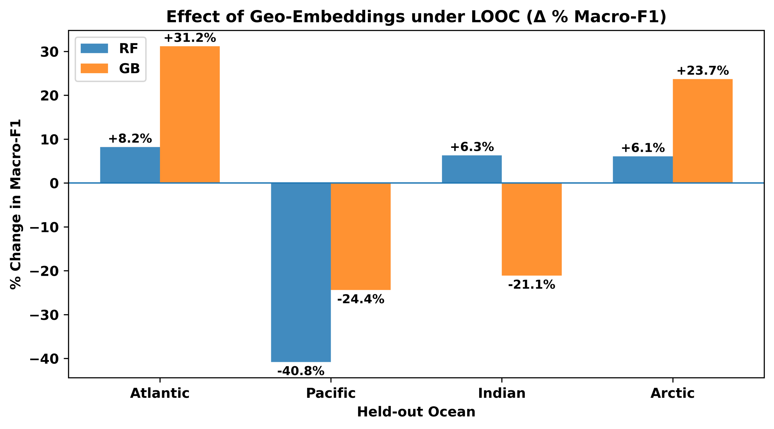
Table 3 shows that the effect of geo-embeddings is strongly domain-dependent: performance improves in the Atlantic (+31 %, p < 0.001) and the Arctic (+24 %, p < 0.001), degrades in the Pacific (−24 %, p < 0.001) and shows no statistically significant change in the Indian Ocean (−21 %, p ≈ 0.58). Figure 5 confirms that this pattern is consistent across Gradient Boosting and Random Forest, suggesting that these effects arise primarily from the representation under distribution shift rather than from a specific ensemble model.
| Ocean | GB (Baseline) | GB + Embed | Effect (mean) | Δ (%) | p-value |
| Atlantic | 0.2010 | 0.2638 | +0.0628 | +31.2 | < 0.001 |
| Pacific | 0.2560 | 0.1934 | −0.0626 | −24.4 | < 0.001 |
| Indian | 0.1779 | 0.1404 | −0.0375 | −21.1 | 0.58 |
| Arctic | 0.1150 | 0.1423 | +0.0273 | +23.7 | < 0.001 |
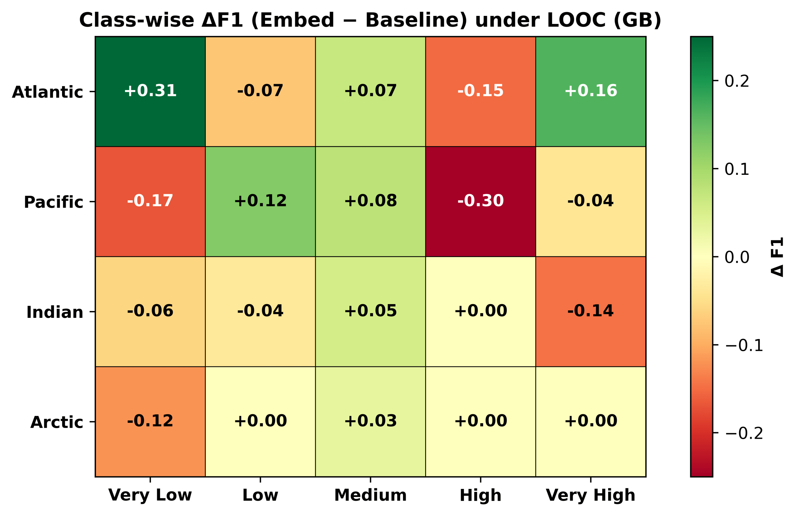
This behavior can be traced to which classes gain and which lose under embeddings, rather than a uniform shift in separability as shown in Figure 6. In the Atlantic, improvements are driven by large gains in Very Low (+0.31) and Very High (+0.16), which outweigh declines in High (−0.15). In contrast, in the Pacific—the most label-diverse domain—embeddings simultaneously degrade Very Low (−0.17) and High (−0.31), while modest gains in Low (+0.12) and Medium (+0.08) are insufficient to compensate. Notably, the Medium class—the largest class in every ocean (≈ 39 – 67 %)—shows consistent improvement across all oceans, suggesting a more consistent embedding–label relationship for this class across domains.
Overall, under LOOCV, geo-embeddings exhibit class and domain-dependent generalization, consistently improving the dominant class while producing domain-dependent effects for other classes—yielding Macro-F1 gains for the Atlantic and Arctic, but degrading Macro-F1 in the Pacific. The degradation in the Pacific stems from its higher label diversity, which is not represented in the training data under LOOCV, requiring generalization to unseen multi-class patterns.
Discussion
Ensemble models such as Random Forest (RF) and Gradient Boosting (GB) consistently outperform SVC, confirming the importance of nonlinear models for this task. RF and GB generally perform similarly, while geo-embeddings produce consistent performance improvements across both models. This task is inherently challenging due to uneven data distribution across oceans and significant class imbalance, which complicate both model learning and evaluation.
At the ocean level, embedding effectiveness varies with label distribution and data availability. The largest gains for both Macro-F1 and Weighted-F1 are observed in the Pacific Ocean, which has the most balanced class distribution, where embeddings improve minority class recognition. In the Atlantic Ocean, improvements are more modest and primarily reflected in Weighted-F1. In contrast, the effects of embeddings in the Arctic and Indian Oceans are smaller and not statistically significant.
These heterogeneous effects are reflected in global aggregation. When averaged across oceans, geo-embeddings yield the largest improvements in Weighted-F1, driven primarily by gains in high-support regions. In contrast, gains in Macro-F1 are smaller and not statistically significant, due to uneven and class-dependent effects across oceans.
The RBF ablation shows that nonlinear transformations of coordinates alone are insufficient to explain embedding gains, as RBF features produce smaller and less consistent improvements. Leave-one-ocean-out evaluation further reveals that embedding performance is domain-dependent under spatial distribution shift. While embeddings improve performance in some domains, such as the Atlantic and Arctic, they degrade performance in others—most notably in the Pacific, the most label-diverse domain. Notably, in this setting, embeddings consistently improve performance for the majority class (Medium) across all oceans, while effects on minority classes are more variable. This suggests that embeddings capture region-specific spatial patterns that do not consistently generalize across oceans with differing class distributions.
This study has several limitations. The dataset is unevenly distributed across oceans, reducing reliability in under-sampled regions such as the Southern Ocean. While geo-embeddings improve performance under standard cross-validation, they do not consistently generalize under distribution shift. Additionally, the models rely primarily on spatial inputs and do not incorporate oceanographic variables such as currents, temperature, or wind, which influence microplastic transport. Finally, the geo-embeddings used in this work are pre-trained and not optimized for the specific prediction task.
Future work should explore hybrid spatial-physical models that combine geo-embeddings with oceanographic variables, as well as domain adaptation and task-specific fine-tuning of embeddings to improve robustness across regions with differing data distributions. Additionally, approaches to address regional imbalance such as ocean-balanced sampling or hierarchical modeling across oceans may further improve balanced performance across regions, although these methods must be applied carefully given extreme data scarcity in certain regions (e.g., the Southern Ocean), which may introduce additional variance or instability.
Despite these limitations, categorical predictions can support targeted monitoring strategies by prioritizing regions predicted to have High or Very High microplastic concentrations for sampling, cleanup, and resource allocation, while reducing effort in low-risk regions predicted to have Low microplastic concentration. This enables more standardized and scalable global monitoring using only widely available inputs.
Conclusion
We present a global framework for predicting ocean microplastic concentration levels using universally available geographic inputs. Ensemble (RF and GB) models outperform SVC, while geo-embeddings produce consistent improvements across both RF and GB models, with the strongest improvements observed in large, diverse oceans such as the Pacific (Marco-F1and Weighted-F1) and the Atlantic (Weighted-F1).
Embedding effectiveness varies across oceans, with stronger gains in class-balanced regions and weaker or inconsistent improvements in imbalanced or data-sparse settings. Globally, embeddings improve performance primarily in Weighted-F1 (≈ 5–8 %), while Macro-F1 gains remain limited due to heterogeneous, class-dependent effects.
The RBF ablation shows that these improvements cannot be explained by nonlinear coordinate transformations alone. Under leave-one-ocean-out evaluation, embedding performance is domain-dependent: improvements are observed in some regions, such as the Atlantic and Arctic, but degrade in others, particularly in label-diverse domains such as the Pacific. Notably, embeddings consistently improve performance for the majority class (Medium) across oceans, contributing to overall gains while limiting improvements in class-balanced metrics.
Overall, pre-trained geo-embeddings improve in-domain performance under standard evaluation but generalize inconsistently under spatial distribution shift, motivating more robust hybrid spatial-physical approaches that combine domain-adapted embeddings with ocean circulation data.
Appendix
Appendix Note: Results for the Southern Ocean are reported for completeness; however, due to extremely limited sample size, they are excluded from aggregate statistical computations.
A. Model Hyperparameters
| Model Variant | Best Hyperparameters |
| SVC (Baseline) | kernel = ‘rbf’, C = 100, gamma = ‘scale’ |
| GB (Baseline) | n_estimators = 300, max_depth = 3, min_samples_leaf = 5 |
| GB (Baseline + Embed) | n_estimators = 300, max_depth = 4, min_samples_leaf = 5 |
| RF (Baseline) | n_estimators = 200, max_depth = 12, min_samples_leaf = 5 |
| RF (Baseline + Embed) | n_estimators = 200, max_depth = 14, min_samples_leaf = 5 |
Per-class Classification Report by Ocean (Gradient Boosting Models)
| Ocean | Class | Precision (Baseline) | Precision (Baseline + Embed) | Recall (Baseline) | Recall (Baseline + Embed) | F1 (Baseline) | F1 (Baseline + Embed) |
| Atlantic | 0 | 0.535±0.027 | 0.531±0.016 | 0.387±0.033 | 0.519±0.008 | 0.449±0.030 | 0.525±0.009 |
| Atlantic | 1 | 0.228±0.008 | 0.241±0.023 | 0.505±0.017 | 0.391±0.039 | 0.314±0.009 | 0.298±0.028 |
| Atlantic | 2 | 0.748±0.016 | 0.756±0.012 | 0.494±0.017 | 0.572±0.018 | 0.595±0.013 | 0.651±0.013 |
| Atlantic | 3 | 0.343±0.015 | 0.375±0.035 | 0.751±0.032 | 0.579±0.039 | 0.470±0.016 | 0.455±0.036 |
| Atlantic | 4 | 0.418±0.046 | 0.428±0.030 | 0.736±0.030 | 0.647±0.051 | 0.532±0.043 | 0.513±0.020 |
| Pacific | 0 | 0.753±0.023 | 0.802±0.020 | 0.761±0.017 | 0.814±0.015 | 0.756±0.008 | 0.808±0.013 |
| Pacific | 1 | 0.557±0.048 | 0.594±0.045 | 0.656±0.037 | 0.658±0.017 | 0.602±0.038 | 0.623±0.024 |
| Pacific | 2 | 0.813±0.007 | 0.828±0.017 | 0.589±0.027 | 0.720±0.019 | 0.683±0.019 | 0.770±0.015 |
| Pacific | 3 | 0.542±0.037 | 0.660±0.040 | 0.866±0.024 | 0.813±0.039 | 0.666±0.034 | 0.729±0.037 |
| Pacific | 4 | 0.557±0.032 | 0.618±0.095 | 0.684±0.042 | 0.685±0.046 | 0.614±0.036 | 0.648±0.068 |
| Indian | 0 | 0.673±0.070 | 0.689±0.113 | 0.540±0.198 | 0.588±0.122 | 0.588±0.146 | 0.625±0.083 |
| Indian | 1 | 0.336±0.413 | 0.209±0.231 | 0.336±0.413 | 0.336±0.413 | 0.336±0.413 | 0.243±0.263 |
| Indian | 2 | 0.863±0.048 | 0.868±0.029 | 0.874±0.043 | 0.881±0.046 | 0.867±0.024 | 0.874±0.019 |
| Indian | 3 | 0.709±0.188 | 0.778±0.146 | 0.813±0.174 | 0.748±0.206 | 0.738±0.120 | 0.733±0.062 |
| Indian | 4 | 0.647±0.191 | 0.830±0.264 | 0.950±0.112 | 0.783±0.217 | 0.749±0.153 | 0.750±0.127 |
| Arctic | 0 | 0.425±0.146 | 0.420±0.129 | 0.250±0.091 | 0.411±0.145 | 0.303±0.098 | 0.403±0.129 |
| Arctic | 1 | 0.000±0.000 | 0.000±0.000 | 0.000±0.000 | 0.000±0.000 | 0.000±0.000 | 0.000±0.000 |
| Arctic | 2 | 0.732±0.056 | 0.719±0.087 | 0.563±0.054 | 0.587±0.119 | 0.634±0.029 | 0.645±0.101 |
| Arctic | 3 | 0.338±0.088 | 0.353±0.118 | 0.608±0.059 | 0.392±0.059 | 0.426±0.060 | 0.366±0.087 |
| Arctic | 4 | 0.575±0.127 | 0.592±0.133 | 1.000±0.000 | 1.000±0.000 | 0.724±0.097 | 0.737±0.105 |
| Southern | 0 | 0.917±0.167 | 0.625±0.479 | 1.000±0.000 | 0.625±0.479 | 0.950±0.100 | 0.625±0.479 |
| Southern | 1 | 0.583±0.500 | 0.583±0.500 | 0.625±0.479 | 0.625±0.479 | 0.542±0.417 | 0.542±0.417 |
| Southern | 2 | 0.933±0.149 | 0.817±0.171 | 0.750±0.250 | 0.800±0.209 | 0.798±0.140 | 0.796±0.156 |
Per Fold Model Performance
| Fold | Group | Macro F1 | Weighted F1 | Total Support |
| 0 | Arctic Ocean | 0.4406 | 0.4542 | 64 |
| 0 | Atlantic Ocean | 0.4076 | 0.4340 | 1969 |
| 0 | Indian Ocean | 0.5560 | 0.6110 | 107 |
| 0 | Pacific Ocean | 0.5398 | 0.5537 | 1099 |
| 0 | Southern Ocean | 0.3333 | 0.3333 | 2 |
| 1 | Arctic Ocean | 0.3494 | 0.3778 | 56 |
| 1 | Atlantic Ocean | 0.4089 | 0.4237 | 2017 |
| 1 | Indian Ocean | 0.6056 | 0.6626 | 99 |
| 1 | Pacific Ocean | 0.5083 | 0.5322 | 1063 |
| 1 | Southern Ocean | 0.4444 | 0.2222 | 6 |
| 2 | Arctic Ocean | 0.2537 | 0.3298 | 68 |
| 2 | Atlantic Ocean | 0.4521 | 0.4594 | 1981 |
| 2 | Indian Ocean | 0.6297 | 0.6496 | 102 |
| 2 | Pacific Ocean | 0.5327 | 0.5540 | 1084 |
| 2 | Southern Ocean | 0.4889 | 0.7111 | 6 |
| 3 | Arctic Ocean | 0.3838 | 0.4658 | 63 |
| 3 | Atlantic Ocean | 0.4101 | 0.4286 | 1907 |
| 3 | Indian Ocean | 0.5659 | 0.5999 | 116 |
| 3 | Pacific Ocean | 0.5306 | 0.5658 | 1149 |
| 3 | Southern Ocean | 1.0000 | 1.0000 | 6 |
| 4 | Arctic Ocean | 0.3442 | 0.4789 | 59 |
| 4 | Atlantic Ocean | 0.4335 | 0.4445 | 1994 |
| 4 | Indian Ocean | 0.4693 | 0.5650 | 121 |
| 4 | Pacific Ocean | 0.5183 | 0.5533 | 1060 |
| 4 | Southern Ocean | 0.3333 | 0.4286 | 7 |
| Fold | Group | Macro F1 (Baseline) | Weighted F1 (Baseline) | Macro F1 (Baseline + Embed) | Weighted F1 (Baseline + Embed) | Total Support |
| 0 | Arctic | 0.5081 | 0.5324 | 0.4603 | 0.5805 | 64 |
| 0 | Atlantic | 0.4570 | 0.4967 | 0.4653 | 0.5342 | 1969 |
| 0 | Indian | 0.6750 | 0.8221 | 0.6230 | 0.7904 | 107 |
| 0 | Pacific | 0.6688 | 0.6928 | 0.7329 | 0.7621 | 1099 |
| 0 | Southern | 1.0000 | 1.0000 | 1.0000 | 1.0000 | 2 |
| 1 | Arctic | 0.3577 | 0.4398 | 0.3548 | 0.4642 | 56 |
| 1 | Atlantic | 0.4679 | 0.4982 | 0.4744 | 0.5458 | 2017 |
| 1 | Indian | 0.8392 | 0.8430 | 0.7362 | 0.8320 | 99 |
| 1 | Pacific | 0.6576 | 0.6810 | 0.7211 | 0.7436 | 1063 |
| 1 | Southern | 0.7222 | 0.6944 | 0.3571 | 0.4643 | 6 |
| 2 | Arctic | 0.4056 | 0.5036 | 0.4139 | 0.4691 | 68 |
| 2 | Atlantic | 0.4802 | 0.5101 | 0.5068 | 0.5595 | 1981 |
| 2 | Indian | 0.6401 | 0.7799 | 0.5858 | 0.7578 | 102 |
| 2 | Pacific | 0.6405 | 0.6753 | 0.6993 | 0.7613 | 1084 |
| 2 | Southern | 0.8286 | 0.8381 | 0.6250 | 0.6667 | 6 |
| 3 | Arctic | 0.4336 | 0.5169 | 0.4848 | 0.6028 | 63 |
| 3 | Atlantic | 0.4576 | 0.5039 | 0.4944 | 0.5524 | 1907 |
| 3 | Indian | 0.5834 | 0.7528 | 0.6236 | 0.7859 | 116 |
| 3 | Pacific | 0.6668 | 0.6914 | 0.7096 | 0.7541 | 1149 |
| 3 | Southern | 0.5556 | 0.7778 | 0.6190 | 0.9048 | 6 |
| 4 | Arctic | 0.4229 | 0.5665 | 0.4374 | 0.5583 | 59 |
| 4 | Atlantic | 0.4968 | 0.5225 | 0.5009 | 0.5692 | 1994 |
| 4 | Indian | 0.5635 | 0.7270 | 0.6567 | 0.8006 | 121 |
| 4 | Pacific | 0.6649 | 0.6967 | 0.7148 | 0.7613 | 1060 |
| 4 | Southern | 0.8222 | 0.8476 | 0.8222 | 0.8476 | 7 |
| Fold | Group | Macro F1 (Baseline) | Weighted F1 (Baseline) | Macro F1 (Baseline + Embed) | Weighted F1 (Baseline + Embed) | Total Support |
| 0 | Arctic | 0.4639 | 0.6195 | 0.4588 | 0.6021 | 64 |
| 0 | Atlantic | 0.4559 | 0.4954 | 0.4761 | 0.5289 | 1969 |
| 0 | Indian | 0.6582 | 0.8374 | 0.6752 | 0.8232 | 107 |
| 0 | Pacific | 0.6862 | 0.7017 | 0.7264 | 0.7572 | 1099 |
| 0 | Southern | 1.0000 | 1.0000 | 1.0000 | 1.0000 | 2 |
| 1 | Arctic | 0.3011 | 0.4079 | 0.3402 | 0.4190 | 56 |
| 1 | Atlantic | 0.4668 | 0.4976 | 0.4726 | 0.5325 | 2017 |
| 1 | Indian | 0.7345 | 0.8235 | 0.7264 | 0.7813 | 99 |
| 1 | Pacific | 0.6689 | 0.6892 | 0.6984 | 0.7305 | 1063 |
| 1 | Southern | 0.6000 | 0.5000 | 0.7222 | 0.6944 | 6 |
| 2 | Arctic | 0.3633 | 0.4334 | 0.3889 | 0.4493 | 68 |
| 2 | Atlantic | 0.4801 | 0.5098 | 0.5152 | 0.5627 | 1981 |
| 2 | Indian | 0.6379 | 0.7958 | 0.6316 | 0.7718 | 102 |
| 2 | Pacific | 0.6717 | 0.7126 | 0.7135 | 0.7633 | 1084 |
| 2 | Southern | 0.3333 | 0.6667 | 0.8286 | 0.8381 | 6 |
| 3 | Arctic | 0.4504 | 0.5380 | 0.5002 | 0.6236 | 63 |
| 3 | Atlantic | 0.4565 | 0.5028 | 0.4855 | 0.5470 | 1907 |
| 3 | Indian | 0.6127 | 0.7583 | 0.5974 | 0.7332 | 116 |
| 3 | Pacific | 0.6775 | 0.7011 | 0.7142 | 0.7583 | 1149 |
| 3 | Southern | 0.5556 | 0.8889 | 1.0000 | 1.0000 | 6 |
| 4 | Arctic | 0.4122 | 0.5439 | 0.4305 | 0.5576 | 59 |
| 4 | Atlantic | 0.4957 | 0.5218 | 0.4959 | 0.5558 | 1994 |
| 4 | Indian | 0.6425 | 0.7820 | 0.6085 | 0.7359 | 121 |
| 4 | Pacific | 0.6967 | 0.7233 | 0.7198 | 0.7640 | 1060 |
| 4 | Southern | 0.2250 | 0.3286 | 0.8222 | 0.8476 | 7 |
Ocean-wise Embedding Effect for GB (relative to GB Baseline)
Fold-wise effects are calculated using data from Table C2. Confidence Intervals (CIs) are obtained using 1000 bootstrap samples from the fold-wise embedding effect table for both Macro-F1 and Weighted-F1. p-values are computed using the Wilcoxon signed-rank test on paired fold-level differences.
| Fold | Atlantic | Pacific | Indian | Arctic | Southern |
| 0 | +0.0084 | +0.0640 | -0.0521 | -0.0478 | +0.0000 |
| 1 | +0.0065 | +0.0635 | -0.1030 | -0.0029 | -0.3651 |
| 2 | +0.0266 | +0.0588 | -0.0543 | +0.0082 | -0.2036 |
| 3 | +0.0368 | +0.0428 | +0.0401 | +0.0512 | +0.0635 |
| 4 | +0.0040 | +0.0499 | +0.0932 | +0.0146 | +0.0000 |
| Ocean | GB (Baseline) | GB (Baseline + Embed) | Effect (Mean) | Effect (95% CI) | p-value | % Gain (Mean) |
| Atlantic | 0.4719 | 0.4884 | +0.0165 | [+0.006, +0.027] | 0.0625 | +3.49 |
| Pacific | 0.6597 | 0.7155 | +0.0558 | [+0.047, +0.065] | 0.0312 | +8.46 |
| Indian | 0.6603 | 0.6451 | -0.0152 | [-0.066, +0.034] | 0.4375 | -2.30 |
| Arctic | 0.4256 | 0.4302 | +0.0046 | [-0.034, +0.043] | 0.8125 | +1.08 |
| Fold | Atlantic | Pacific | Indian | Arctic | Southern |
| 0 | +0.0374 | +0.0693 | -0.0317 | +0.0482 | +0.0000 |
| 1 | +0.0477 | +0.0627 | -0.0109 | +0.0243 | -0.2302 |
| 2 | +0.0494 | +0.0860 | -0.0221 | -0.0345 | -0.1714 |
| 3 | +0.0485 | +0.0627 | +0.0331 | +0.0859 | +0.1270 |
| 4 | +0.0467 | +0.0645 | +0.0736 | -0.0082 | +0.0000 |
| Ocean | GB (Baseline) | GB (Baseline + Embed) | Effect (Mean) | Effect (95 % CI) (95% CI) | p-value | % Gain (Mean) |
| Atlantic | 0.5063 | 0.5522 | +0.0459 | [+0.038, +0.052] | 0.0312 | +9.07 |
| Pacific | 0.6874 | 0.7565 | +0.0691 | [+0.062, +0.077] | 0.0312 | +10.05 |
| Indian | 0.7849 | 0.7933 | +0.0084 | [-0.026, +0.045] | 0.6250 | +1.07 |
| Arctic | 0.5118 | 0.5350 | +0.0232 | [-0.020, +0.068] | 0.3125 | +4.53 |
Ocean-wise Embedding Effect for RF (relative to RF Baseline)
Fold-wise effects are calculated using data from Table C3. Confidence Intervals (CIs) and p-values are obtained using the same procedure as in D.
| Fold | Atlantic | Pacific | Indian | Arctic | Southern |
| 0 | +0.0202 | +0.0402 | +0.0170 | -0.0051 | +0.0000 |
| 1 | +0.0058 | +0.0295 | -0.0081 | +0.0391 | +0.1222 |
| 2 | +0.0351 | +0.0418 | -0.0063 | +0.0256 | +0.4952 |
| 3 | +0.0290 | +0.0367 | -0.0153 | +0.0498 | +0.4444 |
| 4 | +0.0002 | +0.0231 | -0.0340 | +0.0183 | +0.5972 |
| Ocean | RF (Baseline) | RF (Baseline + Embed) | Effect (Mean) | Effect (95 % CI) (95% CI) | p-value | % Gain (Mean) |
| Atlantic | 0.4708 | 0.4890 | +0.0181 | [+0.006, +0.031] | 0.0625 | +3.85 |
| Pacific | 0.6802 | 0.7144 | +0.0343 | [+0.025, +0.045] | 0.0312 | +5.04 |
| Indian | 0.6572 | 0.6479 | -0.0093 | [-0.028, +0.010] | 0.4375 | -1.42 |
| Arctic | 0.3982 | 0.4237 | +0.0255 | [-0.002, +0.052] | 0.1250 | +6.40 |
| Fold | Atlantic | Pacific | Indian | Arctic | Southern |
| 0 | +0.0335 | +0.0555 | -0.0142 | -0.0174 | +0.0000 |
| 1 | +0.0349 | +0.0413 | -0.0422 | +0.0111 | +0.1944 |
| 2 | +0.0529 | +0.0507 | -0.0240 | +0.0159 | +0.1714 |
| 3 | +0.0442 | +0.0572 | -0.0251 | +0.0856 | +0.1111 |
| 4 | +0.0340 | +0.0407 | -0.0461 | +0.0137 | +0.5190 |
| Ocean | RF (Baseline) | RF (Baseline + Embed) | Effect (Mean) | Effect (95 % CI) (95% CI) | p-value | % Gain (Mean) |
| Atlantic | 0.5055 | 0.5453 | +0.0399 | [+0.030, +0.051] | 0.0312 | +7.90 |
| Pacific | 0.7056 | 0.7546 | +0.0491 | [+0.041, +0.058] | 0.0312 | +6.96 |
| Indian | 0.7994 | 0.7691 | -0.0303 | [-0.045, -0.015] | 0.0312 | -3.79 |
| Arctic | 0.5085 | 0.5303 | +0.0218 | [-0.018, +0.063] | 0.3125 | +4.29 |
Effect of Month feature on Gradient Boosting (GB) Model Prediction
Baseline model uses latitude, longitude and ocean as features and the alternative model uses month as an additional feature. Confidence Intervals (CIs) and p-values using the same process as in D using the corresponding fold-wise effect tables.
| Ocean | Δ (Macro-F1) | CI (Macro-F1) | p-value (Macro-F1) | Δ (Weighted-F1) | CI (Weighted-F1) | p-value (Weighted-F1) |
| Atlantic | +0.0096 | [−0.002, +0.018] | 0.12 | +0.0060 | [−0.002, +0.012] | 0.15 |
| Pacific | +0.0145 | [+0.002, +0.025] | 0.06 | +0.0068 | [+0.001, +0.013] | 0.08 |
| Indian | +0.0466 | [−0.010, +0.100] | 0.31 | +0.0351 | [−0.005, +0.070] | 0.25 |
| Arctic | +0.0006 | [−0.010, +0.010] | 0.75 | −0.0055 | [−0.015, +0.005] | 0.50 |
G. Global Embedding Effect
Confidence Intervals (CIs) and p-values are obtained using the same procedure as in D. Fold-wise global effect is obtained by aggregating (sample-wt. and equal-wt.) model performance across oceans from tables C2 and C3.
| Fold | RF (equal wt.) | RF (sample-wt.) | GB (equal-wt.) | GB (sample-wt.) |
| 0 | +0.018075 | +0.01461 | -0.006875 | +0.01807 |
| 1 | +0.016575 | +0.01082 | -0.008975 | +0.01605 |
| 2 | +0.024050 | +0.01650 | +0.009825 | +0.01588 |
| 3 | +0.025050 | +0.01968 | +0.042725 | +0.02336 |
| 4 | +0.001900 | -0.01306 | +0.040425 | +0.00592 |
| Metric | RF (equal-wt.) | RF (sample-wt.) | GB (equal-wt.) | GB (sample-wt.) |
| Mean Δ | +0.0171 | +0.0097 | +0.0154 | +0.0159 |
| 95% CI (Δ) | [0.006, 0.025] | [-0.010, 0.019] | [-0.009, 0.041] | [0.006, 0.023] |
| p-value | 0.0625 | 0.1250 | 0.3125 | 0.0625 |
| Fold | RF (equal-wt.) | RF (sample-wt.) | GB (equal-wt.) | GB (sample-wt.) |
| 0 | +0.014350 | +0.02931 | +0.030800 | +0.04150 |
| 1 | +0.011275 | +0.01688 | +0.030950 | +0.03884 |
| 2 | +0.023875 | +0.02810 | +0.019700 | +0.03342 |
| 3 | +0.040475 | +0.03092 | +0.057550 | +0.03763 |
| 4 | +0.010575 | +0.03039 | +0.044150 | +0.05244 |
| Metric | RF (equal-wt.) | RF (sample-wt.) | GB (equal-wt.) | GB (sample-wt.) |
| Mean Δ | +0.0201 | +0.0271 | +0.0366 | +0.0408 |
| 95% CI (Δ) | [0.010, 0.035] | [0.018, 0.032] | [0.025, 0.050] | [0.034, 0.048] |
| p-value | 0.0625 | 0.0312 | 0.0312 | 0.0312 |
References
- M. Eriksen, L. C. M. Lebreton, H. S. Carson, M. Thiel, C. J. Moore, J. C. Borerro, F. Galgani, P. G. Ryan, and J. Reisser, “Plastic pollution in the world’s oceans: More than 5 trillion plastic pieces weighing over 250,000 tons afloat at sea,” PLOS ONE, vol. 9, no. 12, e111913, 2014. 2014. http://doi.org/10.1371/journal.pone.0111913 [↩]
- K. L. Law, S. Moret-Ferguson, N. A. Maximenko, G. Proskurowski, E. E. Peacock, J. Hafner, and C. M. Reddy, “Plastic accumulation in the North Atlantic subtropical gyre,” Science, vol. 329, no. 5996, pp. 1185–1188, 2010. http://doi.org/10.1126/science.1192321 [↩]
- A. Cózar, F. Echevarría, J. I. González-Gordillo, X. Irigoien, B. Úbeda, S. Hernández-León, Á. T. Palma, S. Navarro, J. García-de-Lomas, A. Ruiz, M. L. Fernández-de-Puelles, and C. M. Duarte, “Plastic debris in the open ocean,” Proc. Natl. Acad. Sci. USA, vol. 111, no. 28, pp. 10239–10244, 2014. http://doi.org/10.1073/pnas.1314705111 [↩]
- N. Maximenko, J. Hafner, and P. Niiler, “Pathways of marine debris derived from trajectories of Lagrangian drifters,” Marine Pollution Bulletin, vol. 65, no. 1–3, pp. 51–62, 2012. https://doi.org/10.1016/j.marpolbul.2011.04.016 [↩]
- L. C. M. Lebreton, J. van der Zwet, J.-W. Damsteeg, B. Slat, A. Andrady, and J. Reisser, “River plastic emissions to the world’s oceans,” Nature Communications, vol. 8, 15611, 2017. https://doi.org/10.1038/ncomms15611 [↩]
- E. van Sebille, C. Wilcox, L. Lebreton, N. Maximenko, B. D. Hardesty, J. A. van Franeker, M. Eriksen, D. Siegel, F. Galgani, and K. L. Law, “A global inventory of small floating plastic debris,” Environmental Research Letters, vol. 10, no. 12, 124006, 2015. https://doi.org/10.1088/1748-9326/10/12/124006 [↩]
- X. Yan, Z. Cao, A. Murphy, and Y. Qiao, “An ensemble machine learning method for microplastics identification with FTIR spectrum,” Journal of Environmental Chemical Engineering, vol. 10, no. 4, 108130, 2022. https://doi.org/10.1016/j.jece.2022.108130 [↩]
- N. Meyers, B. De Witte, N. Schmidt, D. Herzke, J.-L. Fuda, D. Vanavermaete, C. R. Janssen, and G. Everaert, “From microplastics to pixels: Testing the robustness of two machine learning approaches for automated, Nile Red-based marine microplastic identification,” Environmental Science and Pollution Research, vol. 31, pp. 61860–61875, 2024. https://doi.org/10.1007/s11356-024-35289-0 [↩]
- S. Primpke, C. Lorenz, R. Rascher-Friesenhausen, and G. Gerdts, “An automated approach for microplastics analysis using focal plane array (FPA) FTIR microscopy and image analysis” , Analytical Methods, vol. 9, no. 9, pp. 1499–1511, 2017. https://doi.org/10.1039/C6AY02476A [↩]
- M. E. Mihailov, A. V. Chiroșca, E. D. Pantea, and G. Chiroșca, “Machine learning approaches for microplastic pollution analysis in Mytilus galloprovincialis in the Western Black Sea,” Sustainability, vol. 17, no. 12, 5664, 2025. https://doi.org/10.3390/su17125664 [↩]
- H. T. Tran, M. Hadi, T. T. Nguyen, H. G. Hoang, M. T. Nguyen, K. T. H. Nguyen, and D.-V. N. Vo, “Machine learning approaches for predicting microplastic pollution in peatland areas,” Marine Pollution Bulletin, vol. 194, 115417, 2023. https://doi.org/10.1016/j.marpolbul.2023.115417 [↩]
- H. Dong, R. Zhang, X. Wang, J. Zeng, L. Chai, X. Niu, L. Xu, Y. Zhou, P. Gong, and Q. Yin, “Geographical features and management strategies for microplastic loads in freshwater lakes,” npj Clean Water, vol. 8, 29, 2025. https://doi.org/10.1038/s41545-025-00459-1 [↩]
- X. Jin, Z. Li, J. Peñuelas, Q. Wu, Y. Peng, P. Heděnec, C. Yuan, J. Yuan, Z. Chen, Z. Zhao, F. Wu, and K. Yue, “Quantitative assessment on the distribution patterns of microplastics in global inland waters,” Communications Earth & Environment, vol. 6, 331, 2025. https://doi.org/10.1038/s43247-025-02320-2 [↩]
- X. X. Zhu, D. Tuia, L. Mou, G.-S. Xia, L. Zhang, F. Xu, and F. Fraundorfer, “Deep learning in remote sensing: A comprehensive review and list of resources,” IEEE Geoscience and Remote Sensing Magazine, vol. 5, no. 4, pp. 8–36, 2017. https://doi.org/10.1109/MGRS.2017.2762307 [↩]
- M. Belgiu and L. Drăguț, “Random forest in remote sensing: A review of applications and future directions,” ISPRS Journal of Photogrammetry and Remote Sensing, vol. 114, pp. 24–31, 2016. https://doi.org/10.1016/j.isprsjprs.2016.01.011 [↩]
- M. Reichstein, G. Camps-Valls, B. Stevens, M. Jung, J. Denzler, N. Carvalhais, and Prabhat, “Deep learning and process understanding for data-driven Earth system science,” Nature, vol. 566, pp. 195–204, 2019. https://doi.org/10.1038/s41586-019-0912-1 [↩]
- D. R. Roberts, V. Bahn, S. Ciuti, M. S. Boyce, J. Elith, G. Guillera-Arroita, S. Hauenstein, J. J. Lahoz-Monfort, B. Schröder, W. Thuiller, D. I. Warton, B. A. Wintle, F. Hartig, and C. F. Dormann, “Cross-validation strategies for data with temporal, spatial, hierarchical, or phylogenetic structure,” Ecography, vol. 40, no. 8, pp. 913–929, 2017. https://doi.org/10.1111/ecog.02881 [↩]
- N. Jean, M. Burke, M. Xie, W. M. Davis, D. B. Lobell, and S. Ermon, “Combining satellite imagery and machine learning to predict poverty,” Science, vol. 353, no. 6301, pp. 790–794, 2016. https://doi.org/10.1126/science.aaf7894 [↩]
- N. Jean, S. Wang, A. Samar, G. Azzari, D. Lobell, and S. Ermon, “Tile2Vec: Unsupervised representation learning for spatially distributed data,” in Proceedings of the AAAI Conference on Artificial Intelligence, vol. 33, no. 1, pp. 3967–3974, 2019. https://doi.org/10.1609/aaai.v33i01.33013967 [↩]
- G. Mai, K. Janowicz, Y. Hu, S. Gao, B. Yan, R. Zhu, L. Cai and N. Lao “A review of location encoding for geoAI: Methods and applications,” International Journal of Geographical Information Science, vol. 36, no. 11, pp. 2289–2322, 2022. https://doi.org/10.1080/13658816.2021.2004602 [↩]
- K. Klemmer, E. Rolf, C. Robinson, L. Mackey, and M. Rußwurm, “SatCLIP: Global, general-purpose location embeddings with satellite imagery,” in Proceedings of the AAAI Conference on Artificial Intelligence, vol. 39, no. 4, pp. 4347–4355, 2025. https://doi.org/10.1609/aaai.v39i4.32457 [↩]
- K. Ayush, B. Uzkent, C. Meng, M. Burke, D. Lobell, and S. Ermon, “Geography-aware self-supervised learning,” in Proceedings of the IEEE/CVF International Conference on Computer Vision (ICCV), pp. 10181–10190, 2021. https://doi.org/10.1109/ICCV48922.2021.01002 [↩]
- C. Bodnar, W. P. Bruinsma, A. Lucic, M. Stanley, A. Allen, J. Brandstetter, P. Garvan, M. Riechert, J. A. Weyn, H. Dong, J. K. Gupta, K. Thambiratnam, A. T. Archibald, C.-C. Wu, E. Heider, M. Welling, R. E. Turner and P. Perdikaris, “A foundation model for the Earth system, ” Nature 641, 1180–1187, 2025. https://doi.org/10.1038/s41586-025-09005-y [↩]
- E. S. Nyadjro, J. A. B. Webster, T. P. Boyer, J. Cebrian, L. Collazo, G. Kaltenberger, K. Larsen, Y. H. Lau, P. Mickle, T. Toft, and Z. Wang, “The NOAA NCEI marine microplastics database,” Scientific Data, vol. 10, 726, 2023. https://doi.org/10.1038/s41597-023-02632-y [↩]
- C. Cortes and V. Vapnik, “Support-vector networks,” Machine Learning, vol. 20, no. 3, pp. 273–297, 1995. https://doi.org/10.1007/BF00994018 [↩]
- L. Breiman, “Random forests,” Machine Learning, vol. 45, no. 1, pp. 5–32, 2001. https://doi.org/10.1023/A:1010933404324 [↩]
- J. H. Friedman, “Greedy function approximation: A gradient boosting machine,” The Annals of Statistics, vol. 29, no. 5, pp. 1189–1232, 2001. https://doi.org/10.1214/aos/1013203451 [↩]
- F. Pedregosa, G. Varoquaux, A. Gramfort, V. Michel, B. Thirion, O. Grisel, M. Blondel, P. Prettenhofer, R. Weiss, V. Dubourg, J. VanderPlas, A. Passos, D. Cournapeau, M. Brucher, M. Perrot, and É. Duchesnay, “Scikit-learn: Machine learning in Python,” Journal of Machine Learning Research, vol. 12, pp. 2825–2830, 2011 [↩]