Comparing First-Order and Second-Order Markov Chains for Algorithmic Melody Generation

Abstract

Markov chain models are a well-established probabilistic approach in algorithmic music composition. This study examines whether increased contextual memory improves the local coherence of algorithmically generated melodies in a limited setting by comparing first-order and second-order Markov chain approaches to monophonic melody generation. Both models were trained on a simplified version of Minuet in G by Petzold, represented as separate pitch and rhythm token sequences. Pitch and rhythm were modelled independently using empirical transition probabilities and recombined to generate fixed-length melodies of 16 notes. Each model produced seventy-five melodies. Objective evaluation combined a weighted music-theory-based scorecard assessing tonic resolution, interval smoothness, stepwise motion, motivic repetition, and rhythmic variety, together with comparison against a random baseline. Subjective evaluation used a blinded listening survey completed by 15 participants. In the objective evaluation, the second-order model achieved the highest final scores, both Markov models outperformed the random baseline, and the second-order model showed a small advantage over the first-order model. In the subjective evaluation, second-order melodies received higher ratings for pleasantness and overall quality, while coherence and randomness showed the same directional pattern but were not statistically significant after correction. These findings suggest that increased contextual memory may offer a modest benefit for short-range melodic organization in Markov-based music generation under the conditions of this study, which was based on a single training piece and a limited sample.

Keywords: Algorithmic music composition, Markov chains, melody generation, computational creativity, probabilistic modelling

Introduction

Algorithmic music composition refers to the use of computational methods to generate music. A central challenge in this field is the modelling of musical coherence in ways that resemble human composition, particularly in melody generation. One of the earlier works in algorithmic music composition was GenJam, which applied a genetic algorithm with human fitness evaluation to generate jazz solos¹.

More recent reviews show that the field has expanded considerably, encompassing probabilistic systems, neural networks, hybrid approaches, and rule-guided methods. Duraisamy et al., for example, provide a comparative overview of approaches including Markov chains, recurrent neural networks, GANs, variational encoders, and Transformer-based models, and report high accuracy for Transformer-based systems². Within this broader landscape, Markov-related approaches remain relevant because they explicitly model the probability of one musical event following another. This makes them well suited to examining how local sequential dependency influences generated melodic structure.

Schulze and van der Merwe compared Markov chains of varying orders with hidden Markov models and found that HMMs (Hidden Markov Models) captured melody-chord relationships effectively but showed limitations in rhythm, rests, and multiple voices. They also reported that mixed-order Markov chains tended to produce shorter sequences, whereas higher-order models generated longer and more structured outputs³.

Related work on probabilistic models further suggests that design choices such as chord representation can affect melodic prediction performance across HMM-based and IOHMM-based models⁴. Hill observed that melodies generated by 0th- and 2nd-order Markov chains were perceived as more interesting than those generated by 1st- or 3rd-order models⁵.

Related work has explored extensions or neighbouring probabilistic frameworks. Chen et al. adapt Markovian ideas through random forest regression, demonstrating that lightweight sequence-based models can still generate accessible monophonic melodies⁶ (single-note melodies without harmony).

Tsushima et al. proposed a hierarchical generative model combining a probabilistic context-free grammar for chord syntax with Markov models for chord rhythms and pitch sequences, outperforming conventional HMM-based harmonization in melody prediction and chord sequence accuracy⁷. Nakamura et al. incorporate music-theoretic hierarchy into a probabilistic model of monophonic music, while Temperley shows that meter, harmony, and stream structure can be jointly represented within a unified probabilistic framework^8,9. Boulanger-Lewandowski et al. further show that richer sequence models such as RNN-RBM outperform simpler N-gram and Markov baselines on most datasets¹⁰.

Beyond Markov-based music generation, the literature includes a wide range of different approaches designed to capture longer-range structure, richer texture, or greater flexibility. Choi et al. show that LSTM networks can learn musical patterns from text-like symbolic representations, although their evaluation is largely informal¹¹. DeepBach represents a more developed example, combining a steerable deep architecture with a large-scale listening experiment to assess generated chorales¹².

GAN-based and Transformer-based systems extend generation into more complex and polyphonic settings. MuseGAN, for instance, focuses on multi-track symbolic music generation and combines objective metrics with listener evaluation¹³. A related polyphonic generation study combines a GAN framework with Markov decision process for policy gradient optimization¹⁴. Another study combines GAN adversarial learning with transformer architecture for music Adversarial Transformer (ATM)¹⁵.

More recent work has also introduced rule-guided diffusion for symbolic music generation, enabling non-differentiable musical constraints (such as note density, chord progression) to control a pre-trained diffusion-based model without retraining¹⁶. A Transformer-XL-based study applies cross-domain pre-training from Lakh MIDI to NES-style symbolic music generation and reports lower perplexity and stronger user-study performance than unigram, 5-gram, and LSTM baselines¹⁷.

A multimodal study introduces V-MusProd, a three-stage Transformer framework for chord, melody, and accompaniment generation conditioned on video semantic, colour, and motion features, and reports better performance than the CMT baseline on both correspondence and music-quality metrics¹⁸. Additionally, a study introduces a motif-to-music framework combining motif-level repetition generation with outline-to-music generation, and shows that explicit modelling of repetition improves both objective repetition matching and subjective ratings of musical quality¹⁹.

A hybrid approach further combines machine learning with rule-based approach, allowing user-defined musical constraints to guide generated outputs independently of training style²⁰. Other methods include a genetic algorithm using Normalized Compression Distance (NCD) as a fitness function²¹.

A task-specific probabilistic system for guitar solo generation combines HMM-based phrase detection, bigram models for rhythm and pitch in tablature space, chord-tone preference, and ornament modelling, with listener tests showing significant gains from these musically informed components²². Context-aware systems such as StemGen that generate music in response to existing audio input, and style-based approaches such as Cruz’s classifier framework for identifying composer similarity in RNN-generated music are other approaches^23,24.

Although these models often achieve stronger performance on complex tasks, they typically require larger datasets, more computational resources, and more advanced implementation. By contrast, Markov models remain attractive where transparency, simplicity, and low computational cost are important, particularly in smaller-scale or educational research settings.

Evaluation is an important consideration in this literature. Urbano et al. argue that evaluation in music information retrieval often lacks validity, reliability, and efficiency, with weak corpora, missing baselines, and limited statistical analysis remaining common problems²⁵. Agres, Forth, and Wiggins similarly argue that meaningful assessment of computational creativity should combine objective and subjective approaches rather than rely on only one form of evidence²⁶.

In practice, subjective listener surveys remain a commonly used evaluation method in algorithmic composition studies. Schulze and van der Merwe, for example, reported that 72% of participants were either unable to distinguish between human-composed and Markov-generated melodies or preferred the computer-generated outputs³.

Objective, music-theory-based evaluation remains relatively less common. Cruz uses a classifier to assess composer-style similarity in RNN-generated music, while Shapiro and Huber analyse Markov-generated compositions through theoretical similarities to training material, such as scale usage and pitch relationships^27,28. Hahn et al. incorporate music-theory considerations during generation, although they do not propose a fully developed objective evaluation framework²⁹.

Additionally, MuseGAN was assessed using metrics such as empty bars, used pitch classes, qualified notes, drum patterns, and tonal distance while Zhang used measures including unique pitch and duration counts, short-pattern repetitions, and concurrent note counts for objective evaluation of the ATM mode^30,15.

Particularly relevant in this context is Guo et al.’s evaluation method, which combines statistical analysis with music-theory-based metrics such as smooth-saltatory progression, wave test and note-level mode test³¹.

This line of work suggests that generated symbolic music can be assessed not only through generic numerical similarity measures or listener preference alone, but also through musically interpretable structural features. For the present study, this suggests that a mixed evaluation design may be appropriate, with objective music-theory-based analysis used to examine differences between outputs and subjective listening used to assess whether those differences are perceptually meaningful.

A Markov chain is a probabilistic process in which the likelihood of a future state depends on one or more previous states. In music generation, each state typically represents a musical event, such as a note or pitch. In a first-order Markov chain, the probability of the next state depends only on the current state³². Thus, the Markov model has a memory of one preceding event. This is given by:

   

Here, denotes the transition probability from state to state . For all values of , the choice of the next note depends solely on the immediately preceding note.

In contrast, a second-order Markov chain considers a longer context as it has a memory of two preceding events rather than one. Here, the probability of the next state depends on the two preceding states, allowing the model to capture short sequences rather than isolated transitions⁷. This relationship is represented as:

   

denotes the second-order transition probability from the ordered state pair to state .

As discussed previously, a limitation in some existing research on algorithmic melody generation is the limited use of objective, theory-based evaluation methods. Many studies primarily rely on subjective listener judgments, such as perceived pleasantness, without explicitly assessing whether the generated melodies follow fundamental principles of music theory.

Addressing this aspect may enable a more structured evaluation of algorithmic composition methods. In particular, applying a music-theory-based scorecard can provide a framework for objective assessment of melodic features such as interval usage, repetition, and tonal resolution. When combined with subjective listener feedback, this approach offers a more comprehensive understanding of melodic quality.

In light of this, this study investigates the differences between first-order and second-order Markov chain models in melody generation. The models are evaluated using both a music theory scorecard and a listener survey to examine aspects of melodic coherence and overall musical quality within the scope of this work.

Research Question

How do first-order and second-order Markov chain models differ in producing coherent melodies within a constrained experimental setting, as examined by a music theory scorecard and a listener survey?

Hypothesis

It is hypothesised that melodies generated using second-order Markov chains may exhibit higher local coherence than those generated using first-order Markov chains in both objective and subjective evaluations, as including additional contextual information may support more consistent melodic transitions.

Methods

This study employed a comparative, quasi-experimental research design to evaluate differences in melodic coherence between first-order and second-order Markov chain models. The analysis was cross-sectional, with all melodies generated and evaluated within a single study period. A mixed-methods approach was used, combining objective music-theory-based evaluation with subjective listener evaluations to assess coherence and perceived musical quality.

Minuet in G by Petzold (previously attributed to Bach)³³ was chosen as the training piece for this model due to its simplicity and clarity. It is a Classical piece composed for the piano in G major.

Certain changes were made to the original training melody to train the model: the melody was simplified by removing ornamentation such as trills and mordents. Bar structure was eliminated and notes were tokenised into flattened sequences. Additionally, harmonies were removed to keep the melody monophonic (single-note melody without harmony).

Pitch and rhythm were modelled separately using independent Markov chains and combined afterward. Thus, pitch–rhythm dependency was not modelled, so the models never learn joint patterns of pitch-rhythm combinations

Two melody generator programs were implemented using Python: a first-order Markov chain and a second-order Markov chain. Transition probabilities were calculated using the observed frequencies of token sequences in the dataset. New sequences were then generated by sampling from these learned probability distributions.

Both models generated fixed-length sequences of 16 pitches and 16 durations, which were then paired position-by-position into melody events. In addition to these two Markov-generated sets, a random melody set of the same fixed length was included as a baseline for the objective evaluation. The models generated 75 melodies each, which were exported as JSON files.

 In both Markov models, if a current state (first-order) or state pair (second-order) has no outgoing transitions in the learned table, the algorithm restarts generation from a randomly chosen valid state or state pair.

For the first-order Markov model, the distribution of the next token depends only on the current token. The transition probability from token to token is defined as

   

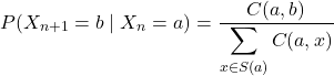
where

   

Here, denotes the number of times token is immediately followed by token in the training data, and the denominator sums counts over all valid next tokens in . In the implementation, corresponds to the set of valid next tokens that have been observed to succeed token present in the learned transition table.

For the second-order Markov model, the distribution of the next token depends on the two preceding tokens. The transition probability is defined as

   

where

   

Here, counts occurrences of the length-3 token pattern in the training data. In this case, corresponds to the set of valid next tokens that have been observed to succeed token pair present in the learned second-order transition table.

 A random seed has been set in the generation process for research replication.

Rhythm was represented as numeric beat values and pitch as note–octave tokens (for example, C5, E4, F#4). The data representation used in generation excludes rests and flats, and is limited to pitch material present in the training melody; these assumptions are detailed further in the evaluation section.

All code used for melody generation and evaluation, along with the exact generated melodies are provided as supplementary material.

Evaluation

Objective Evaluation

To objectively evaluate the melodies, a scorecard based on music theory principles was used.

The evaluator validates pitch tokens against the dataset pitch set and converts notes to MIDI for interval computation (pitch distance between two notes). Pitch tokens in note–octave format (for example, C5 or F#4) were mapped to standard MIDI note numbers, in which each semitone corresponds to an increment of 1.

 Each melody was scored using five criteria (tonic ending, interval smoothness, stepwise motion, motif repetition, and rhythmic variety). Rests and flats are not supported in this evaluation version. These criteria are further explained below.

Rationale Behind Criteria

Ending on the tonic: In classical music, ending a melody on the tonic (central note of a key) provides a sense of completion and stability. It confirms the key and creates a clear feeling of resolution for the listener.

Interval smoothness: Excessive wide leaps can make a melody sound disjointed and difficult to follow. Smaller intervals lead to smoother melodic contours and are characteristic of classical-style melodies.

Preference for stepwise motion: Stepwise motion, defined as movement by one or two semitones, helps maintain melodic continuity and balance.

Motivic repetition: Repetition of short melodic patterns strengthens coherence and makes melodies memorable.

Rhythmic variety: If all notes have the same duration, a melody may sound monotonous; on the other hand, excessive rhythmic variation can reduce clarity. Balanced rhythmic variety maintains listener engagement without overwhelming the listener.

Criterion	Description	Evaluation Approach
Ending on tonic	Melody ends on tonic note of key (central note of the key)	Heuristic key inference (D/G major) from pitch-class counts in final 8 notes; score is 1 if final note is inferred tonic, else 0.
Interval smoothness	Avoids large leaps (big note intervals)	Continuous penalty based on the proportion of melodic intervals exceeding 7 semitones.
Stepwise motion ratio	Uses mainly stepwise movement (note movement by 2 semitones or less)	Continuous score based on the proportion of melodic intervals of 2 semitones or less.
Motif repetition	Recognizable short patterns (motifs) recur	Mean of pitch-based and interval-based motif repetition scores derived from repeated non-trivial sub-sequences.
Rhythmic Variety	Controlled variation of rhythmic values	Combined measure of normalized duration entropy and rhythmic pattern structure.

Objective Score Formulation

The objective evaluation was formulated using continuous or binary measures scaled to the range . Let the final objective score for a melody be denoted by . Since all five criteria were assigned equal importance, the final score was computed as

   

where , , , and represent the scores for ending on tonic, interval smoothness, stepwise motion, motif repetition, and rhythmic variety, respectively.

Ending on tonic

The ending-on-tonic score was treated as a binary indicator of cadential closure. Let the tonic inferred by the key-identification heuristic be denoted by , and let the final note of the melody be . Then

   

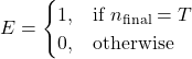
The tonic was inferred heuristically from pitch-class frequencies in the final eight notes, assuming either D major or G major.

Interval smoothness

Interval smoothness was intended to reward melodies that avoid excessive large leaps. Let denote the number of melodic intervals greater than 7 semitones, and let denote the total number of melodic intervals in the melody. The interval smoothness score was defined as

   

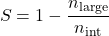
Thus, melodies with fewer large leaps received higher scores.

Stepwise motion

Stepwise motion was measured as the proportion of melodic intervals that were stepwise in nature. Let denote the number of intervals with absolute size less than or equal to 2 semitones. Then

   

Higher values of indicate a greater degree of conjunct melodic motion.

Motif repetition

Motif repetition was used to capture recurrence of short melodic ideas. In the scorecard, this criterion was restricted to melodic structure only, so that rhythmic repetition was handled separately under rhythmic variety.

Two sub-scores were computed: a pitch-based motif score  and an interval-based motif score , each defined using coverage and pattern strength of repeated non-trivial sub-sequences.

Pitch-motif score

Let the pitch sequence be . Repeated pitch patterns of length were identified as sub-sequences occurring at least twice, not allowing overlaps. A pattern was considered non-trivial if it contained at least two distinct pitch values.

Let denote the number of notes belonging to repeated non-trivial pitch patterns. The coverage term was defined as

   

Let , and denote the numbers of distinct repeated non-trivial pitch patterns of lengths 2, 3, and 4, respectively. The pattern strength term was defined as

   

The pitch-motif score was then computed as

   

Interval-motif score

Let the interval sequence be , where

   

Repeated interval patterns of length were identified similarly, with non-trivial patterns defined as those containing at least two distinct interval values.

Let denote the number of intervals belonging to repeated non-trivial interval patterns. The coverage term was defined as

   

Let , and denote the numbers of distinct repeated non-trivial interval patterns of lengths 2, 3, and 4, respectively. The pattern strength term was defined as

   

The interval-motif score was then computed as

   

Final motif repetition score

The overall motif repetition score was defined as

   

This formulation is intended to capture melodic structure through both pitch-level and interval-level recurrence.

Rhythmic variety

Rhythmic variety was designed to reward both diversity of rhythmic values and rhythmic organization. To avoid over-rewarding excessively random rhythms, this criterion combined a normalized entropy term with a rhythmic pattern score.

Let denote the proportion of notes belonging to rhythmic duration category , and let denote the maximum possible number of distinct rhythmic duration categories permitted in the symbolic representation. In this implementation, was taken as the number of distinct duration values observed across the generated melody sets being evaluated.

The normalized rhythmic entropy was computed as

   

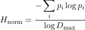
This term captures rhythmic diversity while remaining bounded between 0 and 1.

Next, rhythmic structure was quantified using a rhythmic pattern score, denoted by . Repeated non-trivial rhythmic sub-sequences of length 2 to 4 were identified, where non-trivial patterns were defined as those containing at least two distinct rhythmic values.

Let denote the total number of notes, and let denote the number of notes belonging to repeated non-trivial rhythmic patterns. The coverage term was defined as

   

Let , , and denote the numbers of distinct repeated non-trivial rhythmic patterns of lengths 2, 3, and 4, respectively. The pattern strength term was defined as

   

The rhythmic pattern score was computed as

   

Finally, the rhythmic variety score was defined as

   

This formulation is intended to reflect both diversity of rhythmic values and a degree of structural coherence arising from repeated rhythmic organization.

Additionally, as an initial external check, 15 randomly selected melodies from each of the random baseline, first-order, and second-order sets were also rated by a musician on similar criteria. Associations between objective scores and musician ratings were then examined separately within each model. Because this analysis was based on a single musician and only 15 melodies per set, it is only a preliminary external check and not broader inter-rater reliability

Implementation Notes

Each criterion was scored on a scale from 0 to 1. The final objective score for each melody was calculated as the mean of the five criterion scores. Together, these criteria were intended to represent several complementary aspects of melodic structure, including cadential closure, control of melodic intervals, recurrence of short melodic ideas, and rhythmic diversity with a degree of structural organization.

In motif repetition and rhythmic variety, subsequence lengths of 2–4 were chosen to represent local melodic and rhythmic structure, while limiting the influence of single-element repetition and the relative sparsity of longer patterns.

Additionally, the definition of motivic repetition may favour second-order Markov models, as they condition on two previous notes and are more likely to reproduce short patterns from the training data. Consequently, higher scores on this criterion may partly reflect this structural advantage.

In ‘Ending on Tonic’ criterion, tonic/key handling is heuristic, limited to G and D major as the training melody uses notes only from these key signatures. This simplified mechanism is appropriate for the chosen training material, but it may not scale to passages in other keys, modulating passages or ambiguous tonal centres, and may misclassify some musically plausible endings.Results for each melody were saved in a CSV, with order-wise averages added at the end to facilitate comparison.

Subjective Evaluation

A listening survey was conducted to assess the perceptual quality of generated melodies. A random pre-registered set of three melodies from each Markov order were selected, yielding six monophonic melodies. These were labelled Group A (second-order) and Group B (first-order) for blinded presentation; participants were not informed of the generation method.

Fifteen participants completed the survey via Formester. Participants were from the same school community, and were high-school age. They completed the survey individually on their own devices; listening conditions were therefore not standardised.

At the start, participants self-reported their formal music training level as one of four categories: none, beginner, intermediate, or advanced. Before proceeding, participants confirmed consent to participate in an anonymous school research project. Selecting “No” ended the survey. No personal identifiers were collected.

All melodies were presented in a fixed order with identical instrument (Acoustic Grand Piano) and tempo. After listening, participants responded to four items per melody using a 5-point Likert scale (1 = “Strongly disagree,” 5 = “Strongly agree”):

After rating all six melodies, participants answered a final question: “Overall, which group of melodies sounded more musical? (A or B or no noticeable difference).”

All responses were collected anonymously and exported for analysis.

Statistical Analyses

Statistical analyses were performed separately for the objective and subjective evaluations. For the objective evaluation, differences among the random baseline, first-order, and second-order melody sets were assessed using the Kruskal-Wallis test, followed by pairwise Mann–Whitney U tests with Holm correction for multiple comparisons. For the musician-based validation, Spearman rank correlations were computed separately for the random baseline, first-order, and second-order melody sets. For the subjective evaluation, participant-level mean ratings for Group A and Group B were compared using Wilcoxon signed-rank tests with Holm correction, and overall group preference was assessed using an exact binomial test among participants who expressed a preference. Also, exploratory Spearman correlations were computed between melody-level objective scores and mean listener ratings for the six survey melodies.

Results of both subjective and objective evaluation are provided as supplementary material.

Results

Variable	Order 1 Mean ± SD	Order 1 Median [Q1, Q3]	Order 2 Mean ± SD	Order 2 Median [Q1, Q3]	Random Mean ± SD	Random Median [Q1, Q3]
Ending on tonic	0.24 ± 0.43	0.00 [0.00, 0.00]	0.31 ± 0.46	0.00 [0.00, 1.00]	0.12 ± 0.33	0.00 [0.00, 0.00]
Interval smoothness	0.94 ± 0.06	0.93 [0.93, 1.00]	0.95 ± 0.08	1.00 [0.93, 1.00]	0.63 ± 0.13	0.60 [0.53, 0.73]
Stepwise ratio	0.75 ± 0.12	0.73 [0.67, 0.80]	0.75 ± 0.12	0.73 [0.67, 0.80]	0.26 ± 0.12	0.27 [0.13, 0.33]
Motif repetition	0.32 ± 0.14	0.31 [0.23, 0.39]	0.37 ± 0.16	0.36 [0.27, 0.47]	0.05 ± 0.08	0.00 [0.00, 0.08]
Rhythmic variety	0.56 ± 0.14	0.59 [0.52, 0.65]	0.58 ± 0.10	0.59 [0.54, 0.66]	0.76 ± 0.07	0.77 [0.73, 0.80]
Final score	0.56 ± 0.10	0.54 [0.49, 0.62]	0.59 ± 0.10	0.56 [0.52, 0.64]	0.36 ± 0.08	0.34 [0.32, 0.39]

Table 2 summarizes the descriptive statistics of the objective evaluation measures across the three models. Both Markov models had higher interval smoothness, stepwise ratio, motif repetition, and final score than the random baseline, whereas the random model had the highest rhythmic variety. The second-order model had the highest mean final score (0.59 ± 0.10), followed by the first-order model (0.56 ± 0.10), with the random model scoring lowest (0.36 ± 0.08).

Variable	H	p
Ending on tonic	7.73	0.021
Interval smoothness	148.81	< 0.001
Stepwise ratio	149.14	< 0.001
Motif repetition	129.87	< 0.001
Rhythmic variety	113.37	< 0.001
Final score	123.11	< 0.001

Table 3 shows that overall group differences were statistically significant for all objective evaluation variables. The largest differences were observed for interval smoothness, stepwise ratio, motif repetition, rhythmic variety, and final score (all p < 0.001), while ending on tonic also differed significantly across models (H = 7.73, p = 0.021)

Comparison	U	Adjusted p (Holm)	Rank-biserial correlation	Hodges–Lehmann estimate	95% CI
Order 1 vs Order 2	2274	0.043	-0.191	-0.028	[-0.059, 0.000]
Order 1 vs Random	5287	< 0.001	0.880	0.193	[0.169, 0.221]
Order 2 vs Random	5399	< 0.001	0.920	0.220	[0.204, 0.247]

As shown in Table 4, both Markov models scored significantly higher than the random baseline on the final objective score after Holm adjustment (both p < 0.001). The difference between the first-order and second-order models was much smaller, although still statistically significant (adjusted p = 0.043), with a small effect size.

Results of the exploratory Spearman correlation tests for objective scores and musician ratings indicated that, in the first-order melody set, Ending On Tonic was positively associated with perceived musical resolution (ρ = 0.721, adjusted p = 0.012), Final Score with overall musicality (ρ = 0.806, adjusted p = 0.0017), and Motif Repetition with perceived motifs (ρ = 0.629, adjusted p = 0.048). In the second-order set, Ending On Tonic (ρ = 0.835, adjusted p = 0.00063) and Final Score (ρ = 0.815, adjusted p = 0.0011) likewise showed positive associations with the corresponding musician ratings. No correlation remained statistically significant after Holm correction in the random set.

Melody	Coherence median [Q1, Q3]	Random/disjointedness median [Q1, Q3]	Pleasantness median [Q1, Q3]	Overall rating median [Q1, Q3]	n
A1	3 [2.5, 4]	2 [2, 4]	4 [3, 4.5]	4 [3, 4]	15
A2	3 [2, 4]	2 [1.5, 3]	4 [3, 4.5]	4 [2.5, 4]	15
A3	4 [3, 4]	2 [2, 3]	4 [3, 4]	4 [3, 4]	15
B1	2 [1.5, 3]	4 [2.5, 4]	3 [2, 3]	2 [2, 3]	15
B2	3 [2, 4.5]	3 [1.5, 4]	3 [2, 4]	3 [2.5, 4]	15
B3	3 [1.5, 3.5]	3 [2, 4]	3 [2.5, 4]	3 [2.5, 4]	15

Table 5 summarizes the melody-level listener ratings for the six test melodies. Overall, Group A (second-order) melodies tended to receive higher median ratings for coherence, pleasantness, and overall rating, and lower median ratings for random/disjointedness, than Group B (first-order) melodies.

Criterion	Group A mean	Group B mean	Mean paired difference (A−B)	95% CI for mean difference	W	Adjusted p (Holm)
Coherence	3.356	2.756	0.600	[0.089, 1.111]	18.0	0.051
Randomness	2.400	2.956	−0.556	[−0.911, −0.200]	17.0	0.051
Pleasantness	3.800	3.000	0.800	[0.511, 1.089]	0.0	0.008
Overall rating	3.511	2.889	0.622	[0.244, 1.000]	11.0	0.047

Table 6 presents the participant-level comparisons between Group A and Group B. Group A received higher mean ratings for coherence, pleasantness, and overall rating, while Group B received a higher mean rating for random/disjointedness. After Holm adjustment, the differences were statistically significant for pleasantness (adjusted p = 0.008) and overall rating (adjusted p = 0.047), whereas coherence and randomness showed the same directional pattern but did not remain significant after correction (both adjusted p = 0.051).

Response option	Count	Percentage
Group A	11	73.3
Group B	2	13.3
No noticeable difference	2	13.3

Among participants who expressed a preference (n = 13), 11 preferred Group A and 2 preferred Group B. An exact binomial test indicated that this distribution differed significantly from chance (two-sided p = 0.0225), with more participants preferring Group A.

Fifteen participants had completed the listening survey. Self-reported music-training levels were: none, 6 participants (40.0%); beginner, 3 (20.0%); intermediate, 2 (13.3%); and advanced, 4 (26.7%).

Subjective criterion	Spearman’s ρ	Adjusted p (Holm)
Coherence	0.928	0.0307
Random/disjointedness	-0.696	0.2496
Pleasantness	0.551	0.2574
Overall rating	0.928	0.0307

Additionally, to examine whether the theory-based scorecard was aligned with listener perception, exploratory Spearman rank correlations were computed between melody-level objective scores and mean listener ratings (Table 8). Higher objective scores were associated with higher coherence and overall ratings (both ρ = 0.928, adjusted p = 0.0307). Correlations with lower random/disjointedness and higher pleasantness were in the expected directions, but were not statistically significant after Holm correction. Because these analyses were based on only six melodies, they should be interpreted as exploratory.

Additionally, zero restart events were observed in either first-order or second-order models during sequence generation. The average number of restarts per melody was therefore zero for both models.

Discussion

The findings of this study suggest that second-order Markov chains produced melodies that were generally somewhat stronger than those generated by first-order Markov chains under the present conditions, although the size of this difference depended on the evaluation framework. In the objective evaluation, the second-order model achieved the highest final score, followed by the first-order model, while the random baseline scored lowest. Pairwise comparisons showed that both Markov models scored significantly higher than the random baseline, and that the second-order model also scored higher than the first-order model on the final objective score, although this difference was small. This suggests that conditioning on two preceding notes may offer a modest improvement in local melodic organization rather than a major qualitative shift in output quality.

The inclusion of random melodies as a baseline strengthens this interpretation. Compared with the random model, both Markov models performed substantially better on interval smoothness, stepwise ratio, motif repetition, and final score, suggesting that they captured structural properties not present in arbitrary note sequences. At the same time, the random melodies showed the highest rhythmic variety, indicating that greater surface-level rhythmic variation alone does not necessarily correspond to stronger musical organization within the present scorecard.

The subjective evaluation also favoured the second-order model. Participant-level Wilcoxon signed-rank tests showed significantly higher ratings for pleasantness and overall rating after Holm correction, while coherence and random/disjointedness followed the same directional pattern but were not statistically significant after correction. This suggests that the advantage of the second-order model was reflected most clearly in listeners’ broader judgments of musical appeal and overall impression, rather than equally across every perceptual dimension.

The exploratory correlation analyses provide preliminary support for the theory-based scorecard. As shown in Table 8, higher final objective scores were positively associated with higher mean listener ratings for coherence and overall quality across the six survey melodies. Within the first-order and second-order melody sets, some objective measures were also positively associated with corresponding musician judgments, whereas no correlation remained statistically significant after Holm correction in the random set. Together, these findings suggest that the scorecard was reasonably aligned with perceived musical quality, although the small sample sizes mean that these results should be interpreted cautiously.

Both Markov models also showed no restart events during generation, suggesting that their learned transition structures were sufficiently connected for continuous melody production under the conditions tested. These conclusions remain limited by the use of a single training melody, short generated sequences, and relatively small evaluation samples. Within those limits, however, the results suggest that second-order Markov chains may offer a modest and fairly consistent advantage, while both Markov models produce melodies that are clearly more structured than a random baseline.

Limitations

This study has several limitations that define the scope of its findings. First, both models were trained on a simplified version of Minuet in G, with ornaments removed, bar structure flattened, harmonic information omitted, and the pitch set restricted to that of the source piece. As a result, the findings may not generalize to polyphonic music (involving multiple notes or melodic lines at once), harmonically supported melodies, or other genres and styles.

Second, the study relied on a single training piece and generated fixed-length melodies of 16 notes. Although this allowed controlled comparison between models, it does not show how either model would perform on longer sequences or in generating larger-scale phrase structure, extended motifs, or cadential planning.

Third, pitch and rhythm were modelled independently. This means that the models did not capture joint pitch–rhythm relationships, which are often important to musical structure, and this may have limited their ability to represent more coordinated melodic-rhythmic patterns.

Fourth, the generation and evaluation framework did not include rests, chromatic pitches, or expanded pitch sets beyond those present in the training material. The conclusions therefore apply to a relatively narrow class of simple tonal monophonic melodies.

Fifth, the objective evaluation relied on a heuristic music-theory-based scorecard with predefined criteria and weights. Although the exploratory correlations provided some preliminary support that the scorecard was related to listener judgments, the framework does not capture more complex musical features and should not be treated as a complete measure of musical quality. In particular, the motif-repetition criterion may partly favour second-order Markov models, since conditioning on two previous notes may make short repeated patterns more likely.

Sixth, the subjective evaluation was based on a relatively small listening sample of 15 participants, and the melody-level scorecard–survey correlations were based on only six survey melodies. The musician-based validation correlations were also exploratory and based on 15 melodies per set. These analyses therefore provide only limited evidence about the relationship between objective scores and perceived musical quality and should be interpreted cautiously.

Seventh, in the listening survey, the six melodies were presented in a fixed sequence rather than being randomized or counterbalanced across participants. Order, contrast, or fatigue effects may therefore have influenced ratings, and these effects were not separately controlled or analysed.

Finally, the training melody was flattened without explicit bar separation, and the generated melodies did not include phrase boundaries. Some evaluation criteria refer to coherence and motivic structure, but the generation process itself did not model phrase-level organization. Accordingly, the findings should be interpreted as applying primarily to short-range melodic behaviour rather than to broader musical form.

Despite these limitations, the study provides a structured comparison of first-order, second-order, and random melody generation within a controlled setting. The findings therefore offer preliminary evidence within this limited experimental context, while broader generalization would require more diverse training material, richer representations, and larger evaluation samples.

Supplementary Information

References

1. J. A. Biles. GenJam: a genetic algorithm for generating jazz solos. Proceedings of the International Computer Music Conference (ICMC). Vol. 94, pg. 131-137, 1994. [↩]
2. P. Duraisamy, V. Naveen, G. N. Kishore, S. Nishal. Music generation algorithms: an in-depth review of future directions and applications explored. 2024 IEEE International Conference on Big Data & Machine Learning (ICBDML). pg. 198-203, 2024, https://doi.org/10.1109/ICBDML60909.2024.10577318. [↩]
3. W. Schulze, A. van der Merwe. Music generation with Markov models. IEEE MultiMedia. Vol. 18, pg. 78-85, 2011, https://doi.org/10.1109/MMUL.2010.44. [↩] [↩]
4. J.-F. Paiement, S. Bengio, D. Eck. Probabilistic models for melodic prediction. Artificial Intelligence. Vol. 173, pg. 1266-1274, 2009, https://doi.org/10.1016/j.artint.2009.06.001. [↩]
5. S. Hill. Markov melody generator. Computer Science Department, University of Massachusetts Lowell, 2011. [↩]
6. V. H. H. Chen, J. DeVico, A. Reischer, L. Stepanewk, A. Vasireddy, N. Zhang, S. Dasgupta. Random forest regression of Markov chains for accessible music generation. 2020 IEEE MIT Undergraduate Research Technology Conference (URTC). 2020, https://doi.org/10.1109/URTC51696.2020.9668909. [↩]
7. H. Tsushima, E. Nakamura, K. Itoyama, K. Yoshii. Function- and rhythm-aware melody harmonization based on tree-structured parsing and split-merge sampling of chord sequences. Proceedings of the 18th International Society for Music Information Retrieval Conference (ISMIR 2017). pg. 502-508, 2017, https://archives.ismir.net/ismir2017/paper/000002.pdf. [↩]
8. E. Nakamura, M. Hamanaka, K. Hirata, K. Yoshii. Tree-structured probabilistic model of monophonic written music based on the generative theory of tonal music. 2016 IEEE International Conference on Acoustics, Speech and Signal Processing (ICASSP). pg. 276-280, 2016, https://doi.org/10.1109/ICASSP.2016.7471680. [↩]
9. D. Temperley. A unified probabilistic model for polyphonic music analysis. Journal of New Music Research. Vol. 38, pg. 3-18, 2009, https://doi.org/10.1080/09298210902928495. [↩]
10. N. Boulanger-Lewandowski, Y. Bengio, P. Vincent. Modeling temporal dependencies in high-dimensional sequences: application to polyphonic music generation and transcription. Proceedings of the 29th International Conference on Machine Learning (ICML). pg. 1881-1888, 2012, https://icml.cc/2012/papers/590.pdf. [↩]
11. K. Choi, G. Fazekas, M. Sandler. Text-based LSTM networks for automatic music composition. arXiv. 2016, https://doi.org/10.48550/arXiv.1604.05358. [↩]
12. G. Hadjeres, F. Pachet, F. Nielsen. DeepBach: a steerable model for Bach chorales generation. Proceedings of the 34th International Conference on Machine Learning. Vol. 70, pg. 1362-1371, 2017, https://proceedings.mlr.press/v70/hadjeres17a.html. [↩]
13. H. W. Dong, W. Y. Hsiao, L. C. Yang, Y. H. Yang. MuseGAN: multi-track sequential generative adversarial networks for symbolic music generation and accompaniment. Proceedings of the AAAI Conference on Artificial Intelligence. Vol. 32, pg. 34-41, 2018, https://doi.org/10.1609/AAAI.V32I1.11312. [↩]
14. W. Huang, Y. Xue, Z. Xu, G. Peng, Y. Wu. Polyphonic music generation generative adversarial network with Markov decision process. Multimedia Tools and Applications. Vol. 81, pg. 29865-29885, 2022, https://doi.org/10.1007/S11042-022-12925-W. [↩]
15. N. Zhang. Learning adversarial transformer for symbolic music generation. IEEE Transactions on Neural Networks and Learning Systems. Vol. 34, pg. 1754-1763, 2020, https://doi.org/10.1109/TNNLS.2020.2990746. [↩] [↩]
16. Y. Huang, A. Ghatare, Y. Liu, Z. Hu, Q. Zhang, C. S. Sastry, S. Gururani, S. Oore, Y. Yue. Symbolic music generation with non-differentiable rule guided diffusion. Proceedings of the 41st International Conference on Machine Learning. Vol. 235, pg. 19772-19797, 2024, https://proceedings.mlr.press/v235/huang24g.html. [↩]
17. C. Donahue, H. H. Mao, Y. E. Li, G. W. Cottrell, J. McAuley. LakhNES: improving multi-instrumental music generation with cross-domain pre-training. Proceedings of the 20th International Society for Music Information Retrieval Conference (ISMIR 2019). pg. 685-692, 2019, https://archives.ismir.net/ismir2019/paper/000083.pdf. [↩]
18. L. Zhuo, Z. Wang, B. Wang, Y. Liao, C. Bao, S. Peng. Video background music generation: dataset, method and evaluation. 2023 IEEE/CVF International Conference on Computer Vision (ICCV), Paris, France. pg. 15591-15601, 2023, https://doi.org/10.1109/ICCV51070.2023.01433. [↩]
19. Z. Hu, X. Ma, Y. Liu, G. Chen, Y. Liu, R. B. Dannenberg. The beauty of repetition: an algorithmic composition model with motif-level repetition generator and outline-to-music generator in symbolic music generation. IEEE Transactions on Multimedia. Vol. 26, pg. 4320-4333, 2024, https://doi.org/10.1109/TMM.2023.3321495. [↩]
20. T. Tanaka. Integrating machine learning and rule-based approaches in symbolic music generation. 2024 IEEE International Conference on Big Data (BigData). pg. 3218-3223, 2024, https://doi.org/10.1109/BigData62323.2024.10825900. [↩]
21. M. Alfonseca, A. Cebrian, A. Ortega. A simple genetic algorithm for music generation by means of algorithmic information theory. 2007 IEEE Congress on Evolutionary Computation. pg. 3035-3042, 2007, https://doi.org/10.1109/CEC.2007.4424858. [↩]
22. M. McVicar, S. Fukayama, M. Goto. AutoLeadGuitar: automatic generation of guitar solo phrases in the tablature space. International Conference on Signal Processing Proceedings. pg. 599-604, 2014, https://doi.org/10.1109/ICOSP.2014.7015074. [↩]
23. J. D. Parker, J. Spijkervet, K. Kosta, F. Yesiler, B. Kuznetsov, J.-C. Wang. STEMGEN: a music generation model that listens. ICASSP 2024 – 2024 IEEE International Conference on Acoustics, Speech and Signal Processing (ICASSP). pg. 1116-1120, 2024, https://doi.org/10.1109/ICASSP48485.2024.10446088. [↩]
24. J. Cruz. Deep learning vs Markov model in music generation. Honors College thesis, Pace University, 2019, https://digitalcommons.pace.edu/honorscollege_theses/333. [↩]
25. J. Urbano, O. Schedl, X. Serra, P. Herrera. Evaluation in music information retrieval. Journal of Intelligent Information Systems. Vol. 41, pg. 267-297, 2013, https://doi.org/10.1007/S10844-013-0249-4. [↩]
26. K. Agres, J. Forth, G. A. Wiggins. Evaluation of musical creativity and musical metacreation systems. Computers in Entertainment. Vol. 14, pg. 1-33, 2016, https://doi.org/10.1145/2967506. [↩]
27. J. Cruz. Deep learning vs Markov model in music generation. Honors College thesis, Pace University, 2019, https://digitalcommons.pace.edu/honorscollege_theses/333. [↩]
28. I. Shapiro, M. Huber. Markov chains for computer music generation. Journal of Humanistic Mathematics. Vol. 11, pg. 167-195, 2021, https://doi.org/10.5642/jhummath.202102.08. [↩]
29. S. Hahn, R. Zhu, S. Mak, C. Rudin, Y. Jiang. An interpretable, flexible, and interactive probabilistic framework for melody generation. Proceedings of the 29th ACM SIGKDD Conference on Knowledge Discovery and Data Mining. pg. 4089-4099, 2023, https://doi.org/10.1145/3580305.3599772. [↩]
30. H. W. Dong, W. Y. Hsiao, L. C. Yang, Y. H. Yang. MuseGAN: multi-track sequential generative adversarial networks for symbolic music generation and accompaniment. Proceedings of the AAAI Conference on Artificial Intelligence. Vol. 32, pg. 34-41, 2018, https://doi.org/10.1609/AAAI.V32I1.11312. [↩]
31. Y. Guo, Y. Liu, T. Zhou, L. Xu, Q. Zhang. An automatic music generation and evaluation method based on transfer learning. PLOS One. Vol. 18, pg. e0283103, 2023, https://doi.org/10.1371/journal.pone.0283103. [↩]
32. E. Fosler-Lussier. Markov models and hidden Markov models: a brief tutorial. Technical report TR-98-041, International Computer Science Institute, 1998. [↩]
33. J. S. Bach. Minuet in G major, BWV Anh. 114. Ed. R. Batka. In Bunte Bühne, 2nd series, pg. 47. Georg D. W. Callwey Kunstwart-Verlag, 1902, https://imslp.org. [↩]