
Abstract
Economists have sophisticated tools to gauge how the economy is doing, but there is no simple way for the public to interpret current economic conditions. Just as thermometers exist to track body temperature and categories exist to measure hurricanes, there needs to be something just as intuitive for the economy. This paper introduces the M-Index, a real-time scale from 0 to 100 that helps people understand the current state of the economy without needing a technical background. The M-Index does not try to predict a recession and does not rely on complex models. It uses 20 publicly available economic indicators in various sectors such as labor, financial markets, and housing, and uses a percentile-based scoring system developed from the last 30 years of historical data. Once constructed, the M-Index was backtested against the three recessions of this century to determine its accuracy in reflecting real-time economic conditions. It accurately captured the differences in magnitude and duration of the downturns. Out of sample testing further showed that the M-Index continued to reflect the economic conditions without relying on hindsight. These findings suggest the M-Index can provide a clearer real-time signal of economic health and provides a transparent and easily interpretable way for the public to assess current economic conditions.
Keywords: economic indicators, macroeconomics, economic health, real-time economic data, economic index, economic thermometer
Introduction
The M-Index is a thermometer for the economy. It is a deterministic, real-time score of the economy ranging from 0 to 100 based on the last 30 years of macroeconomic data. It’s like the human body temperature. The body temperature is usually a clear indicator of how sick someone is. A 100° fever isn’t the same as 103°, and the treatment (medicine, doctor visit, hospitalization, etc.) depends on the specific temperature. The M-Index classifies the health of the economy in the same way. It simply shows where the economy stands right now, based on how today’s data compares to the last 30 years. The goal is to design it for everyday people, not just economists.
The M-Index was created to address two common patterns in existing economic tools. Many widely used tools tend to be complex composite models whose internal workings are not fully transparent or binary recession trackers that signal whether or not a recession is occurring without capturing its severity. Neither of those types of models show people what state the economy actually is in. The M-Index’s goal is to become a tool both rigorous enough to explain how the economy is doing and understandable enough for ordinary people to interpret at a glance.
The M-Index reflects the economy because its different indicators play different roles in showing change in economic conditions. The economy generally strengthens when these factors collectively improve, and it generally contracts when these factors collectively decline. The M-Index summarizes the real-time economic conditions in one clear score by combining these signals into one unified measure.
The intent of this tool is to give a standardized measure of current economic conditions that complements current economic commentary. Since different experts and institutions can reach different conclusions from the same data, a unified, numerical score can give people a consistent reference point. The M-Index’s ultimate goal is to act as a deterministic economic thermometer so that everyone can make better, more informed decisions.
Existing Tools
The National Bureau of Economic Research (NBER) defines a recession as “significant decline in economic activity that is spread across the economy and that lasts more than a few months.” A popular rule of thumb for recessions is two consecutive quarters of negative GDP growth, but NBER does not use a specific numerical formula to determine one. They use three criteria and a variety of monthly indicators to declare recessions with a lag1.
Recession probabilities work very differently from the dates that NBER announces. They are statistical estimates of the chance that the economy will enter a downturn in a specific future window. They are developed using a number of economic and financial variables2.
Tools like the Sahm Rule also exist. The Sahm Rule is a simple tool that uses the unemployment rate to try to predict when a recession is starting, and it triggers when the three-month moving average of the unemployment rate increases by 0.5% or more compared to its lowest value in the previous 12 months3.
The Conference Board Leading Economic Index (LEI) is a composite indicator that is designed to forecast turning points in the U.S. business cycle. It is made as a weighted average of ten leading indicators across multiple categories including labor, manufacturing, housing, financial, and consumer expectations. The LEI is designed to anticipate turning points in the business cycle by approximately seven months and is published monthly as an index level relative to a 2016 base of 1004.
The Chicago Fed National Activity Index (CFNAI) is a coincident indicator of U.S. economic activity5. It is made as a weighted average of 85 monthly indicators across multiple categories including production and income, employment, unemployment, and hours, personal consumption and housing, and sales, orders, and inventories6. A zero value on the index represents the economy expanding at its historical trend rate of growth, while a negative value reflects growth that is below average6. The three-month moving average has historically fallen lower than -0.70 during periods of economic contraction6.
The M-Index is placed within the long-standing tradition of building composite indicators in macroeconomics. Burns & Mitchell (1946) established that business cycles are best understood through the behavior of multiple economic series rather than any single indicator7. Composite indicators today like the Conference Board LEI4 and the Chicago Fed National Activity Index5,6 are based on the same idea, since they are each built as composite aggregates of distinct macroeconomic series into one summary measure. The M-Index follows this practice as well by combining indicators across eight sectors of the economy into a single composite score. However, the M-Index reframes the output for non-specialist interpretation using a 0-100 scale and labeled bands.
Issues With Current Economic Tools
Existing economic tools are used by experts, backed by respected institutions, and provide useful information about the state of the economy. However, these tools have limitations that can make them less effective at conveying real-time economic conditions to the general public. In particular, three issues with the current tools have been identified which can reduce their applicability for everyday decision making.
Issue #1: Classification of the Economy
Many of the widely used recession tools categorize the economy as “recession” or “no recession.” But the economy isn’t binary: it is continuous. Over the last 30 years, key indicators of economic health have fluctuated widely: Unemployment Rate ranged from 3.4% to 14.8%, the University of Michigan Consumer Sentiment ranged from 50 to 112, and the Federal Funds Rate ranged from 0.05% to 6.54%8,9,10. That’s not a yes or no scenario, that’s a range. A 7% unemployment rate needs to be treated differently in an economic model than a 10% rate, just like how a 99-degree fever in a person is treated differently than a 103-degree fever. A Category 2 hurricane doesn’t need the same response as a Category 5 hurricane. Economic conditions vary in degree, and measurement tools should reflect that continuous variation.
Issue #2: Usage of Statistical Forecasting
Statistical models depend on robust data, but over the last 50 years, there have been only six recessions (Jan 1980 – Jul 1980, Jul 1981 – Nov 1982, Jul 1990 – Mar 1991, Mar 2001 – Nov 2001, Dec 2007 – Jun 2009, Feb 2020 – Apr 2020)11. That’s just six data points unique in cause and structure. For example, the COVID recession unexpectedly started due to a global pandemic, while the dot-com crash started because of a huge tech collapse. Since recessions’ underlying causes differ, the statistical patterns that are observed in past events may limit the reliability of future downturn predictions. Statistical models generally perform more reliably with larger sample sizes, so an output that “looks accurate” can still be misleading if it’s created using insufficient and weak data.
Issue #3: Accessibility of Existing Tools
Some existing economic tools may be less accessible to non-expert audiences because even when methodology is disclosed, the meaning of their outputs is not self-evident to a general audience. Therefore, non-specialist users, such as workers, families, and small businesses may find it difficult to apply the tools to personal decisions. A related pattern was documented during the post-pandemic period, when the economy performed well according to key economic indicators such as unemployment rate, GDP growth, and wage growth. However, the consumer attitudes about how the economy was performing were different from the economic conditions12, which suggests the interpretation of macroeconomic conditions by the general public is not straightforward, even when underlying indicators are strong.
A composite, real-time economic index works because the economy is not made of just a single variable. Macroeconomic conditions change based on indicators across multiple sectors, and when these sectors weaken at the same time, overall economic performance deteriorates. Conversely, when the sectors strengthen at the same time, the overall economic performance strengthens. An index that captures signals from several independent sectors can provide a more complete representation of the economy than any one indicator.
The M-Index was created to try to address the challenges mentioned above. It is designed to provide a clear and intuitive “snapshot” of the current economy rather than predicting recessions. The M-Index allows everyday people, not just economists, to understand how strong or weak the economy is at a given point in time by synthesizing multiple real-time indicators into a single score.
This study addresses the following research question: Can a composite index built from publicly available macroeconomic indicators differentiate the severity and duration of U.S. economic downturns across historically distinct periods? To address this question, the M-Index is constructed by selecting key macroeconomic indicators, computing a continuous percentile rank for each indicator, and aggregating them into a single composite score. The analysis is limited to US economic data over the last 30 years and is designed to describe current conditions rather than predict future downturns.
Methods
This section explains the M-Index’s development process. This study follows a quantitative, model-building approach with observational backtesting using historical macroeconomic data to construct a real-time composite index. This process had four main stages, which included the following: data sourcing, indicator selection, percentile scoring, aggregation.
Each stage is described on the following pages, and a separate section contains backtesting results.
Stage 1: Data Sourcing
The M-Index is only as good as its data. The Federal Reserve Economic Data (FRED) was used as the primary source because the goal was to create a publicly accessible, replicable tool based on the last 30 years of data (starting April 1995). This is because FRED was a good source for broad macroeconomic coverage, long historical time series, regular, diligent updates, and free public access.
Thus, all historical data used to develop the M-Index except for S&P 500 and Dow Jones data was downloaded from FRED13. S&P 500 and Dow Jones data was downloaded from Macrotrends because FRED only had 10 years of historical data for them and Macrotrends had the necessary 30 years14,15.
To make sure indicators with different reporting frequencies were consistent, all data was standardized to a monthly timeframe. Daily indicators and weekly indicators were aggregated by averaging all values within each month, and monthly indicators were used as is. Quarterly indicators were disaggregated to a monthly frequency by assigning each quarterly value to the three corresponding months, which were then shifted by the publication lag described below (e.g., Q1 values were ultimately applied to April, May, and June). An exception was made for the Equity Market indicators: S&P 500 and Dow Jones monthly closing values were used because daily data was not available from Macrotrends14, and NASDAQ Composite was also aggregated using end-of-period monthly closing values to maintain consistency within the sector.
To prevent future information from leaking onto historical values, indicators with a publication lag over 1 month were lagged to match their approximate release dates. Quarterly indicators (Real GDP16 and Total Debt as a percentage of GDP17) were lagged by 3 months, the Home Price Index (CSUSHPISA)18 was lagged by 2 months, and the Manufacturers’ New Orders (AMTMNO)19 was lagged by 1 month. All other monthly indicators have publication lags under 1 month and were not shifted. These aggregation/disaggregation methods made sure indicators of different frequencies were aligned. Because quarterly indicators were shifted forward by 3 months, the earliest month with a fully computable M-Index value is July 1995, 3 months after the April 1995 start of the analysis window.
Missing data was extremely rare due to FRED’s reliability. Across 360 months for all 20 indicators, fewer than 10 data points in total were missing (<0.2% of all data points). In those instances, the missing indicator was excluded from that month’s composite calculation, and the remaining indicators were averaged.
For some indicators, 6-month percent change was used instead of the raw value, because many factors, such as GDP or home prices, tend to increase naturally over time due to inflation and growth. If the raw values over multiple decades were compared with each other, the recent months would look disproportionally elevated without any actual changes in economic conditions. Using 6-month percent change solves this problem because it normalizes the data over time and thus allows for fairer historical comparison.
Apps Script was used to automate data pulls from FRED API13. Each indicator’s series is fetched through the FRED /series/observations endpoint and written into a dedicated sheet. Missing or non-numeric observations within each pulled series are detected and excluded from the percentile calculation rather than substituted with previous values, which avoids last observation carried forward (LOCF) bias. Failures of the FRED API itself, like timeouts or malformed responses, cause the script to halt and surface the error in the Apps Script execution log, where the script is then re-run after the issue is resolved. While the analysis for this paper was based on data starting in April 1995 and downloaded in April 2026, future versions of the spreadsheet will refresh in real time and will reflect data for subsequent months. One exception: data for High Yield Bond Spread was downloaded in March of 2026 because FRED restricted its historical coverage to 3 years in April of 202620.
Stage 2: Indicator Selection
Indicators across 8 sectors were chosen to span major economic dimensions: Labor Market, Credit Conditions, Monetary Policy, Consumer Demand, Production, Housing, Equity Market, and Structural Health. Indicators were eligible for inclusion in the candidate set if they had monthly-or-better historical data covering substantially all of the April 1995-present analysis window, fit within one of eight pre-specified sectors of the economy, had a known, stable publication lag that could be handled by the lag-adjustment procedure described in Stage 1, so that no future information is used in scoring at any point in time. An initial set of 23 U.S. macroeconomic indicators meeting these criteria was assembled across the 8 sectors.
To ensure the index did not double-count any signals, a full 23×23 Pearson correlation matrix was computed. Any pair with |r| > 0.85 was flagged as redundant. This threshold was selected to ensure any extremely redundant pairs were removed while preserving most indicators across the 8 sectors. The full correlation matrix is provided in the reproducibility supplement. Three pairs exceeded the threshold. High Yield Bond Spread and Corporate Bond Spread (r ≈ 0.93), Durable Goods Orders and Manufacturers’ New Orders (r ≈ 0.93), and the S&P 500 and Dow Jones Industrial Average (r ≈ 0.94). One indicator from each pair was dropped. High Yield Bond Spread was dropped because of FRED’s aforementioned data restriction in April 202620, which prevents future users from reproducing the 30-year percentile scoring. Durable Goods Orders was dropped because it is a subset of Manufacturers’ New Orders. The Dow Jones Industrial Average was dropped in favor of the S&P 500 because the S&P 500 is market-capitalization weighted and broader than the price-weighted Dow21.
After applying this correlation screening, the final M-Index contains 20 indicators. The 20 indicators are distributed across the 8 sectors as follows.
Labor Market (4 indicators) captures employment conditions and labor demand. It includes the Unemployment Rate and its 6-month change (current level and recent trajectory of joblessness), Initial Jobless Claims (the number of people filing for unemployment benefits each week), and Average Weekly Hours in Manufacturing (hours worked per employee in the manufacturing sector).
Credit Conditions (2 indicators) captures the cost and availability of credit. It includes the Corporate Bond Spread (the yield premium of lower-quality corporate bonds over Treasuries) and Bank Credit (the total volume of bank lending).
Monetary Policy (3 indicators) captures monetary policy’s stance as well as inflationary pressure. It includes the Yield Curve (the spread between long and short Treasury yields), the Federal Funds Rate (the central bank’s primary policy interest rate), and CPI (the Consumer Price Index, a measure of consumer-level inflation).
Consumer Demand (2 indicators) captures household spending behavior and confidence in the economy. It includes Advanced Retail Sales (the monthly retail purchasing activity) and the University of Michigan Consumer Sentiment (a survey-based measure of consumer expectations).
Production (2 indicators) captures the real economic output. It includes Industrial Production (the total physical output of factories, mines, and utilities) and Manufacturing New Orders (the dollar value of new orders placed with manufacturers).
Housing (2 indicators) captures the housing sector activity. It includes Building Permits (the number of permits that were issued for new residential construction) and the Case-Shiller Home Price Index (a measure of single-family home values).
Equity Market (2 indicators) captures the conditions in the financial markets. It includes the S&P 500 (an index of 500 of the largest U.S. publicly traded companies) and the NASDAQ Composite (an index weighted toward technology firms).
Structural Health (3 indicators) captures the fiscal conditions in the long term as well as aggregate output. It includes Total Debt as a Percentage of GDP and its 1-year change (the size of federal debt relative to the economy), and Real GDP (the inflation-adjusted total output of the U.S. economy).
Stage 3: Percentile Scoring
The goal of this step is to convert each indicator’s raw value into a normalized score that indicates where the indicator falls on its 30-year historical distribution.
Each month, the score for each indicator comes from calculating its percentile rank against its entire 30-year history. This calculation creates a continuous score from 0-100. The directionality was standardized with a higher score for any particular indicator representing weaker conditions and a lower score representing better conditions. For instance, for unemployment rate, a higher raw value represents a worse economy and thus the raw percentile rank is used as the score as-is. And for GDP, a lower raw value represents a worse economy and thus, 100 minus the percentile rank is used as the score.
When multiple months contain the same indicator value, midpoint tie handling has been used, and it works by averaging the first and last positions of the tied values in the sorted distribution.
This approach was used due to its ability to remove bias in researcher-chosen thresholds and instead rely on the indicator’s 30-year distribution.
Stage 4: Aggregation
The final step in the process of forming the composite M-Index score was the aggregation of all the indicator scores. The previous step explains how each indicator was converted into a 0-100 percentile score; this step explains how the scores were combined.
An equal-weighted average for all 20 indicators was initially considered. However, this method doesn’t account for the different number of indicators in each sector and implicitly gives greater weight to sectors with more indicators. For example, the Labor Market sector has 4 indicators while the Consumer Demand sector only has 2. This method would give a greater weight to labor indicators purely because more indicators were available.
So, a sector-equal weighting scheme was developed. Each of the 20 indicators used in the M-Index is assigned to a sector as mentioned in a previous step. Within each sector, the percentiles of all member indicators are averaged to create a single sector score. The 8 sector scores are then averaged to create the composite M-Index value. This method makes sure that every sector contributes equally to the composite regardless of how many indicators it contains, and it gives each of the 8 major dimensions an equal influence on the final score. This sector-equal approach was chosen because it treats each major dimension of the economy as equally informative.
To support reproducibility, all code, the raw FRED data snapshot, the 23×23 correlation matrix, a per-indicator reference table (FRED code, sector, directionality, publication lag, frequency), and the month-by-month component scores, sector scores, and composite M-Index values are provided in the reproducibility supplement file.
Results
The M-Index uses 20 indicators from 8 economic sectors, which are described in the Indicator Composition by Sector subsection above and listed in the reproducibility supplement. Because each indicator’s score is standardized so that higher scores always represent weakness, a higher composite score represents weaker economic conditions, while a lower score represents stronger economic conditions. The value ranges are: 0–30 excellent, 30–45 normal, 45–60 warning, 60–70 mild stress, 70–80 severe stress, and 80–100 extreme stress. The latter value in each range is exclusive, and the former value is inclusive, except for the top range, which is inclusive of 100.
Boom & Bust Period Backtesting
To validate the M-Index’s behavior across key macroeconomic events of the last 30 years, backtesting was conducted. Claudia Sahm, the creator of the Sahm Rule, validated her tool in this same way22.
Note. Graph created by author
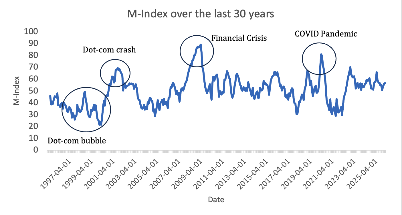
The M-Index was backtested against the three major downturns over the last 30 years (2001, 2008-09, and 2020)11 because they all happened for different reasons (dot-com crash, financial crisis, pandemic). It was also backtested against a boom period over the last 30 years: the dot-com bubble. Figure 1 shows the M-Index over the full 30-year window, with the four periods circled. The shape of the time series shows the index typically remaining below 60 during expansion years, shows the index rising sharply during each labeled downturn, and shows the index falling back below 60 within months of each peak. The diversity in these periods helped ensure the index was valid across different economic periods.
Note. Graph created by author
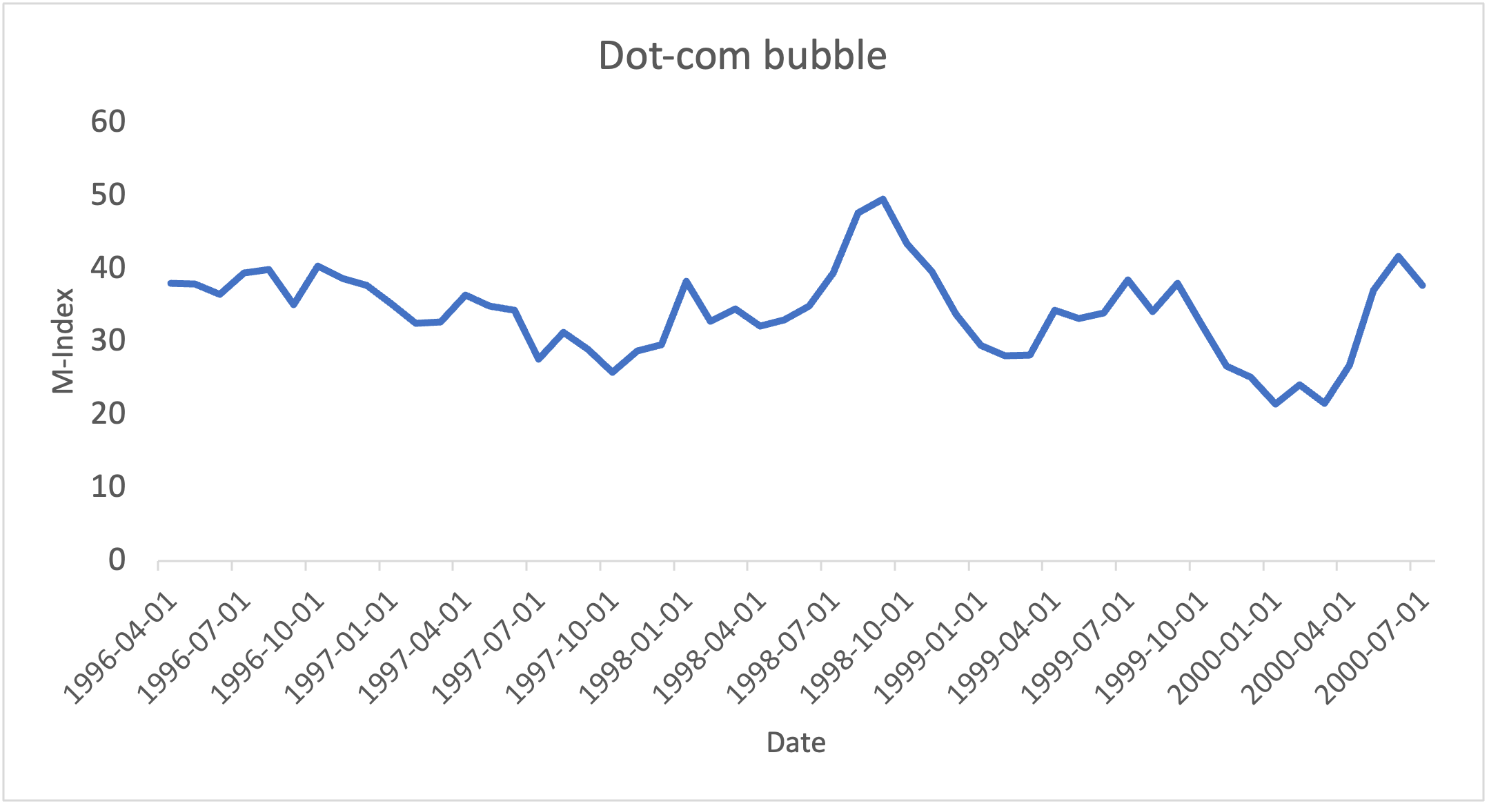
First, the dot-com bubble. As shown in Figure 2, the M-Index ranged from 21.5 to 41.7 between April 1996 to July 2000, with the exception of August to October 1998, when it rose to a peak of 49.5 due to the Russian financial crisis and LTCM collapse23. During this time period, there was heavy speculative investing, a sharp rise in the stock market, and many new internet startups.
Throughout the period, labor indicators such as Unemployment Rate and Initial Jobless Claims, equity indicators such as the SP500 and Nasdaq, and structural health indicators such as GDP performed well. Credit conditions were strong during this period because consumer borrowing expanded. The consistently low scores in multiple indicators within the M-Index reflect healthy economic conditions during the period.
Note. Graph created by author
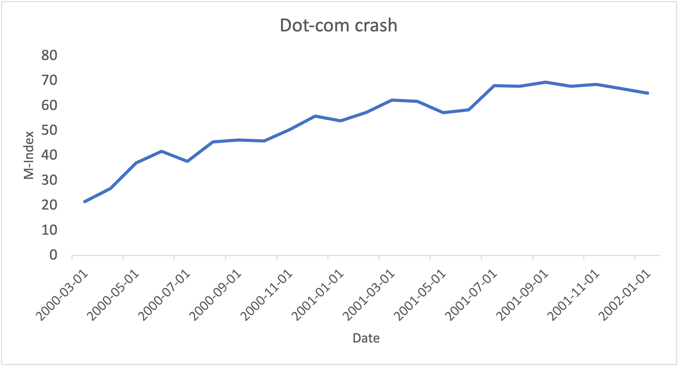
Subsequently, the dot-com crash in 2001. The dot-com bubble burst after a strong economic expansion during the previous few years which ended up triggering the mildest recession in the postwar period24. As Figure 3 shows, the M-Index rose steadily from 21.6 in March 2000 to 62.3 in March 2001. The M-Index peaked at 69.5 in September 2001 and remained ≥ 66.8 from July to December 2001.
During this time, labor indicators such as Initial Jobless Claims and Average Weekly Manufacturing Hours weakened as the job market shrank sharply. The corporate bond spread widened as the borrowing conditions in the overall economy deteriorated. Equity indicators such as major stock indices quickly declined as the economy was contracting as a whole.
Importantly however, the M-Index didn’t reach the severe levels that were observed during the Financial Crisis (max: 89.2) or the COVID pandemic (max: 80.9), which is consistent with the view that this recession was relatively mild. The M-Index’s behavior here indicates its ability to pick up the magnitude of economic stress accurately.
Note. Graph created by author
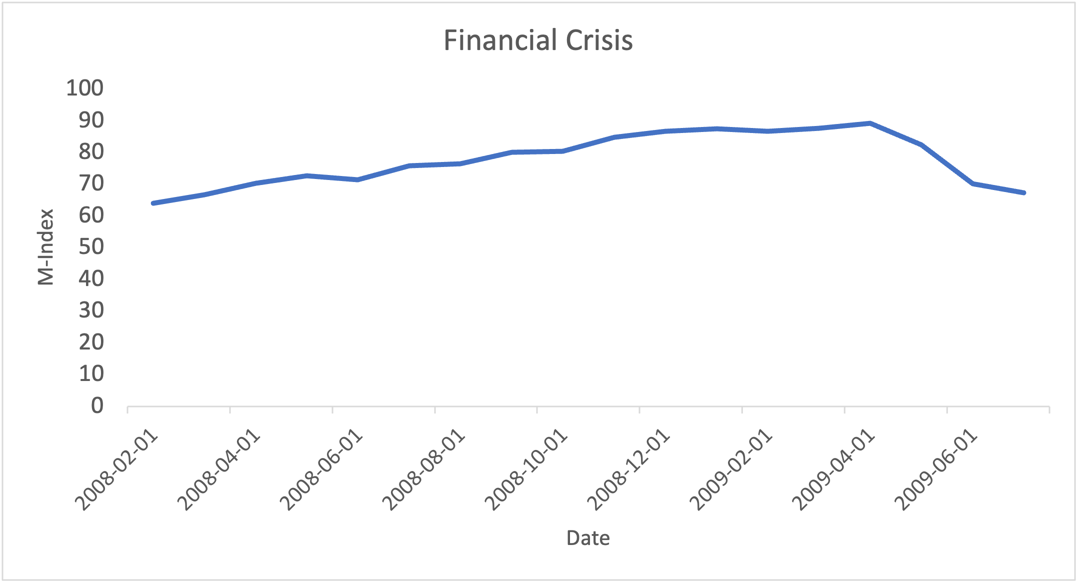
In the ensuing years, the Financial Crisis occurred. This event began in 2008 because of a decrease in housing prices countrywide, and led to a global financial crisis, stock market collapse, and the deepest recession since World War II25. Figure 4 shows a prolonged downturn lasting for approximately 18 months, as the M-Index remained ≥ 63.9 from February 2008 to July 2009, stayed above80 from September 2008 to May 2009, and peaked at 89.2 in April 2009.
The M-Index’s rise during this period was mainly driven by indicators across major sectors weakening. Initially, housing indicators fell sharply which was a sign of stress in the overall economy. The corporate bond spread widened and major stock indices fell, with the S&P500 and Nasdaq severely declining.
The economy suffered in various different areas during the Financial Crisis, and as reflected in the M-Index values, this crisis was more prolonged compared to COVID and reached a higher peak.
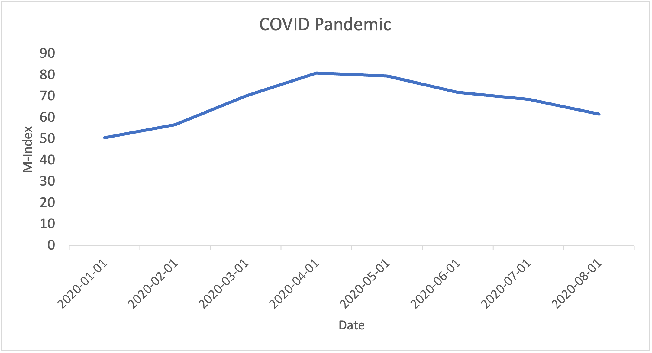
Note. Graph created by author
During the COVID Pandemic, the M-Index sharply jumped by 13.5 (56.7 to 70.2) from February to March 2020. This spike happened because there was a sudden economic shock that caused economic activity to weaken. However, the economy recovered relatively rapidly following a few peak months. During the pandemic, the unemployment rate reached 14.8% in April 2020 and the federal funds rate remained near 0%8,10. As Figure 5 shows, the M-Index peaked at 80.9 in April 2020, and remained at 79.5 in May, before slowly recovering to 71.9 in June, 68.6 in July, and 61.7 in August.
The first indicators to deteriorate during the pandemic were production indicators like Industrial Production26. Also, the GDP declined sharply16, and the Unemployment Rate hit a 30-year high in April 20208. Compared to the Financial Crisis, the COVID downturn was sharper but much shorter, as the M-Index reached a lower peak (80.9 vs. 89.2) but recovered to pre-pandemic levels within 7 months versus 18+ months for the Financial Crisis.
Out of Sample Backtesting
As discussed, the previous backtesting was conducted to understand how the M-Index scored the economy across key macro periods. The in-sample backtesting acts as confirmatory analysis because each indicator’s percentile was calculated using the full 30-year distribution.
So, to provide a more independent evaluation, rolling-origin out of sample backtesting was also conducted. The M-Index score every month was calculated using just the data available until that month. When calculating historical values, no future observations are included since each indicator’s percentile distribution grows by one every month as new data becomes available. This out of sample backtesting was conducted on the 2008 Financial Crisis and the 2020 COVID Pandemic. The dot-com bubble and burst were excluded because of limited pre-period data. The results are shown below.
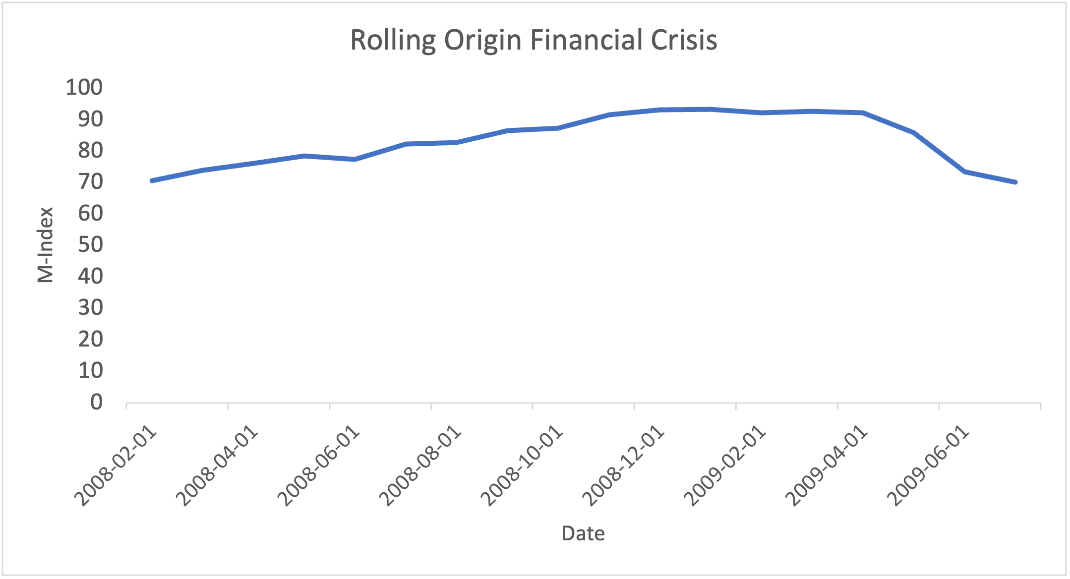
Note. Graph created by author
Note. Graph created by author
Figure 6 shows the rolling-origin M-Index during the Financial Crisis. The index increased between February 2008 (70.5) and November 2008 (91.5) and stayed ≥ 90 until April 2009. The peak of the rolling-origin data (93.2 in January 2009) is slightly higher than and occurred 3 months before the in-sample peak (89.2 in April 2009). This pattern makes sense because the percentile distribution for each month only contained data up to that point, so the crisis was categorized as an extreme event relative to the then-available history. The in-sample methodology includes the full crisis, which produces a lower relative score. One caveat is that the expanding window at this point only contained ~13 years of historical data, which is shorter than the 30-year window the primary M-Index uses. So, the peak value of 93.2 in January 2009 should be interpreted with the understanding that it is computed against less reference data than the in-sample score.
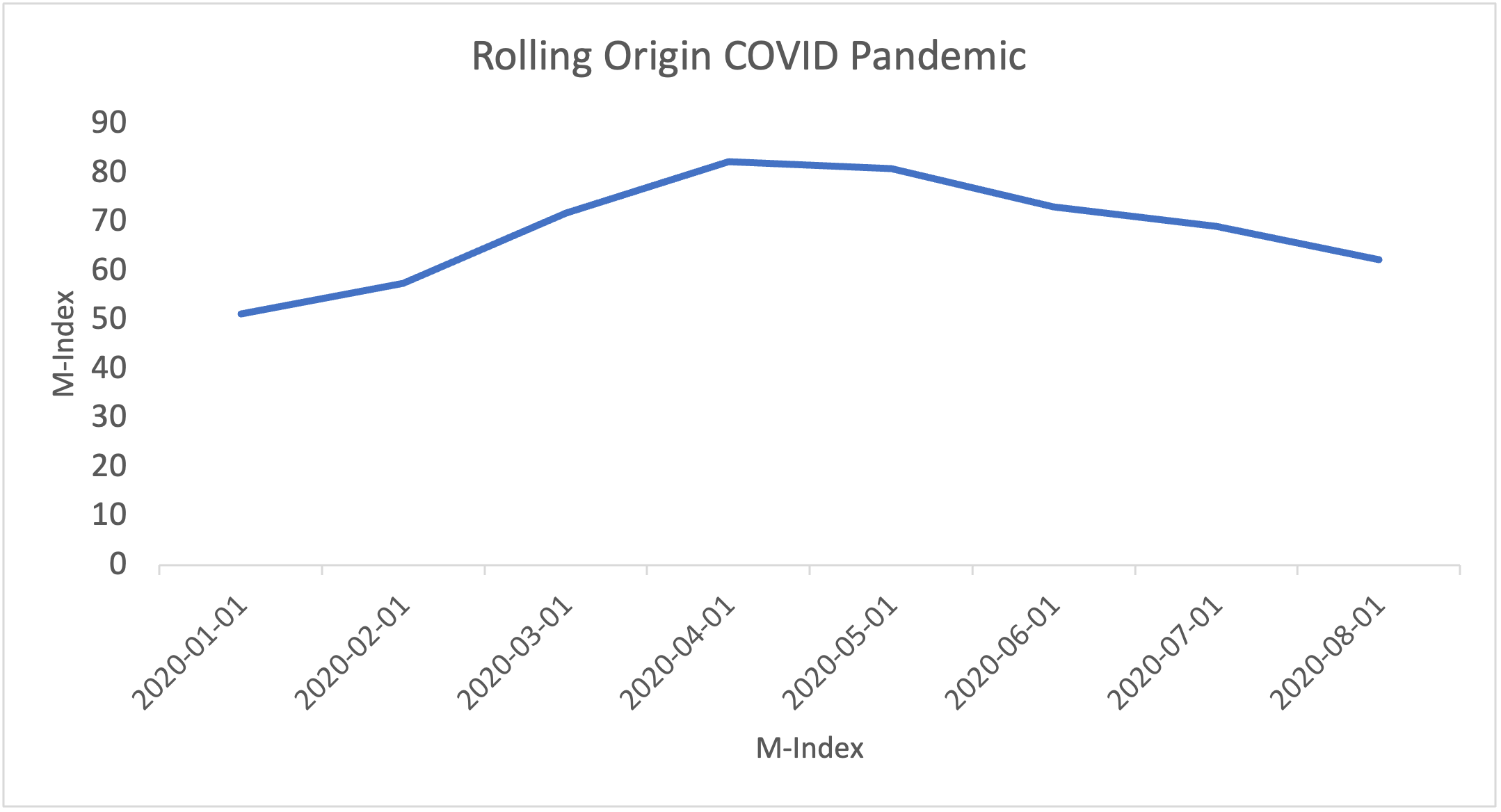
Figure 7 shows the rolling-origin M-Index during the COVID pandemic. The index increased by 14.4 from February 2020 (57.4) to March 2020 (71.8). The index peaked at 82.3 in April 2020, and then slowly declined to 62.2 by August 2020. The peak of the rolling-origin data (82.3) is similar to the in-sample peak (80.9), and both occurred in April 2020. The data values are similar because the reference distribution by early 2020 already contained ~25 out of 30 years of monthly data used in the primary M-Index.
These two backtests show the M-Index was able to pick up on the increased economic stress even without the benefit of hindsight, which indicates that the index reflects real-time economic conditions.
The rolling-origin out-of-sample data, including month-by-month indicator, sector, and composite scores, is provided in a separate reproducibility supplement file.
Validation Across NBER Dates
As an additional structural check, mean M-Index values were calculated across NBER dated recession and expansion months from July 1995 to February 202611. During the 28 months identified by NBER as recessions (dot-com crash, Financial Crisis, and COVID downturn combined), the M-Index averaged 73.6, which falls within the severe stress range. During the remaining expansion months, the M-Index averaged 48.1, which falls within the warning range. The 25.5-point gap indicates that the M-Index values were systematically elevated during NBER-dated recessions relative to expansions.
Discussion
These results indicate that the M-Index differentiates the severity and duration of economic downturns across historically distinct periods, which addresses the research question posed in this study. The in-sample and rolling-origin backtests both had consistent results, which suggests the outputs are not a result of overfitting.
The backtests also show that each downturn had a unique structure. The dot-com crash led to weakness in multiple sectors (labor, credit, equity), but the M-Index only peaked at 69.5 during this time period, supporting the claim that it is the mildest recession in the postwar period24. The Financial Crisis began with a sharp housing decline, which was followed by widened credit spreads and weakened equity markets. During this period, the M-Index remained elevated for 18 months, which shows the depth and duration of the downturn. During COVID, production indicators weakened first, followed by a rapid decline of labor indicators as the M-Index jumped 13.5 points in just one month. Comparisons between different M-Index sectors may be informative as well, because different downturns can produce similar aggregate scores but have very different origins.
It’s also important to clarify exactly what the M-Index is, and exactly what it isn’t. It is a descriptive tool that summarizes the current state of the economy using publicly available macroeconomic data. It is not a forecasting model and does not attempt to predict recessions or estimate their probability. The M-Index is intended to complement existing tools rather than replace them. Recession probability models, the Sahm Rule, and the Conference Board LEI are designed to answer the question of what might happen in the future, while the M-Index and the CFNAI both are designed to answer the question of where the economy stands right now. The M-Index differs from the CFNAI primarily in format and intended audience: the CFNAI uses standard deviation units centered at 0, while the M-Index uses a 0-100 scale with labeled ranges to remain interpretable to people without a technical background. All of these tools answer related but distinct questions, and so the answer to one is not a replacement for the answer to the other.
More broadly, the objective of the M-Index is to present the current state of the economy in a clear way for ordinary people. Instead of trying to simplify the complex economy, this approach turns data from multiple sectors into a single, more comprehensible score. Additional work including user testing still needs to be conducted to determine whether a tool like this meaningfully improves public understanding of economic conditions.
Limitations
While the M-Index provides a structured approach to summarizing the current economic conditions, it is not a perfect solution. Now that it is completed, there are several limitations with the tool.
First, the tool has not been tested with real users. The basis of the tool is that a 0-100 scale with labeled bands is more accessible to non-specialist audiences than the index formats used by existing tools, but this premise has not been empirically validated. A natural next step would be a survey or interview study comparing public interpretation of M-Index values to interpretation of CFNAI or LEI values for the same economic period.
Second, the M-Index is not designed to predict downturns. It is a descriptive tool that summarizes current economic conditions, not a forecasting model. While historical patterns in the M-Index time series may, in retrospect, appear to anticipate downturns, no claim of predictive accuracy is made. Reframing the M-Index as a forecasting tool would require additional methodological work including a defined forecast horizon, an explicit forecast target, and a benchmark against established recession-probability models. This is left as a possible direction for future work.
Third, the in-sample backtesting results were derived with full awareness of the historical economic data, which means they should be interpreted as confirmatory rather than as independent validation. The rolling-origin out of sample COVID and Financial Crisis backtests address this, although the Financial Crisis backtest lacked over half of the historical data (~13 total years).
Fourth, the dot-com crash could not be backtested out of sample because the analysis window begins in 1995, and only ~6 years of pre-period data were available before the March 2001 NBER recession start. As a result, the rolling-origin reference distribution would have been too short for the percentile scoring to be meaningful. The dot-com results in this paper therefore rely on in-sample backtesting only, which is a confirmatory check rather than independent validation. Extending the analysis window further into the past would address this but would require sourcing 30+ years of pre-1995 data for every indicator, which is not consistently available on FRED for all 20 indicators used.
Fifth, although some indicators may have more influence on the economic health, individual indicator weighting was not explored, and equal-sector weighting was implemented instead. Equal-sector weighting treats the major economic sectors as equally important in explaining economic performance, but some indicators such as Unemployment Rate and GDP may have more explanatory power over the economy.
Sixth, formal accuracy metrics were not calculated. The M-Index is designed to be a descriptive tool that explains current economic conditions, so accuracy, prediction error, and other metrics which require a reference outcome for comparison were not applicable. Instead, the M-Index was validated through backtesting against historical downturns over the last 30 years.
Seventh, the M-Index scores are sample-dependent. Each indicator’s percentile rank is computed against the full historical distribution available at the time of scoring, which grows as new data becomes available over time. As a result, rerunning the M-Index in the future will produce slightly different scores for historical months than those reported here, because those monthly indicator values will be ranked against a larger distribution of data. The magnitude of these shifts is expected to be small for established historical months (because each new month adds only ~0.3% to a 30-year reference window), but more material for the most recent months until the distribution stabilizes. Readers should therefore interpret scores in this paper as reflecting the 1995–2026 context window.
Conclusion
Thermometers are used to measure a person’s health. Categories are used to measure hurricanes. There is even an air quality index to measure pollution levels in the atmosphere. However, the economy, which affects every single person, doesn’t have any deterministic, consistent, well understood scale. The M-Index is an attempt at creating one.
Across the dot-com crash, the Financial Crisis, and the COVID downturn, the M-Index reached the Severe stress and Extreme stress bands during the months that NBER later identified as recessions, and averaged 73.6 across NBER-dated recession months versus 48.1 across expansion months. These results, which were validated through both rolling-origin out-of-sample backtesting and the structural NBER comparison, suggest that the M-Index can describe economic conditions across a range of historical environments using a single 0-100 scale.
By providing a continuous score with ordered labels, the M-Index offers a descriptive economic measure that is designed for non-specialist audiences. Whether it ultimately becomes useful in everyday decision-making depends on how individuals choose to interpret and apply it, but the goal is to make the current state of the economy as legible to the public as a thermometer reading.
Supplementary Information
References
- Congressional Research Service. Defining recession. 2024, https://www.congress.gov/crs-product/IF12774. [↩]
- M. T. Owyang, B. Hathhorn. Making sense of recession probabilities. Federal Reserve Bank of St. Louis. 2025, https://www.stlouisfed.org/on-the-economy/2025/may/making-sense-recession-probabilities. [↩]
- Congressional Research Service. The Sahm rule trigger: is the United States in a recession? 2024, https://www.congress.gov/crs-product/IN12410. [↩]
- The Conference Board. US leading indicators. https://www.conference-board.org/topics/us-leading-indicators/. [↩] [↩]
- S. A. Brave, M. Lichtenstein. A different way to review the Chicago Fed National Activity Index. Chicago Fed Letter. No. 298, 2012, https://www.chicagofed.org/publications/chicago-fed-letter/2012/may-298. [↩] [↩]
- Federal Reserve Bank of Chicago. About the Chicago Fed National Activity Index. https://www.chicagofed.org/research/data/cfnai/about. [↩] [↩] [↩] [↩]
- A. F. Burns, W. C. Mitchell. Measuring Business Cycles. National Bureau of Economic Research, 1946, https://www.nber.org/books-and-chapters/measuring-business-cycles [↩]
- U.S. Bureau of Labor Statistics. Unemployment rate. Federal Reserve Bank of St. Louis (FRED). https://fred.stlouisfed.org/series/UNRATE. [↩] [↩] [↩]
- University of Michigan. Consumer sentiment. Federal Reserve Bank of St. Louis (FRED). https://fred.stlouisfed.org/series/UMCSENT. [↩]
- Board of Governors of the Federal Reserve System. Federal funds effective rate. Federal Reserve Bank of St. Louis (FRED). https://fred.stlouisfed.org/series/FEDFUNDS. [↩] [↩]
- National Bureau of Economic Research. U.S. business cycle expansions and contractions. https://www.nber.org/research/data/us-business-cycle-expansions-and-contractions. [↩] [↩] [↩]
- R. Cummings, B. Harris, N. Mahoney. The paradox between the macroeconomy and household sentiment. Brookings Institution. 2024, https://www.brookings.edu/articles/the-paradox-between-the-macroeconomy-and-household-sentiment/. [↩]
- Federal Reserve Bank of St. Louis. FRED database. https://fred.stlouisfed.org/. [↩] [↩]
- Macrotrends. S&P 500 – 100 Year Historical Chart. https://www.macrotrends.net/2324/sp-500-historical-chart-data. [↩] [↩]
- Macrotrends. Dow Jones – 100 Year Historical Chart. https://www.macrotrends.net/1319/dow-jones-100-year-historical-chart. [↩]
- U.S. Bureau of Economic Analysis. Real gross domestic product. Federal Reserve Bank of St. Louis (FRED). https://fred.stlouisfed.org/series/GDPC1. [↩] [↩]
- U.S. Office of Management and Budget. Federal Debt: Total Public Debt as Percent of Gross Domestic Product. Federal Reserve Bank of St. Louis (FRED). https://fred.stlouisfed.org/series/GFDEGDQ188S. [↩]
- S&P Dow Jones Indices LLC. S&P CoreLogic Case-Shiller U.S. national home price index. Federal Reserve Bank of St. Louis (FRED). https://fred.stlouisfed.org/series/CSUSHPISA. [↩]
- U.S. Census Bureau. Manufacturers’ New Orders: Total Manufacturing. Federal Reserve Bank of St. Louis (FRED). https://fred.stlouisfed.org/series/AMTMNO. [↩]
- Ice Data Indices, LLC. ICE BofA US high yield index option-adjusted spread. Federal Reserve Bank of St. Louis (FRED). https://fred.stlouisfed.org/series/BAMLH0A0HYM2. [↩] [↩]
- J. Lin, G. C. Selden, J. B. Shoven, C. Sialm. Replicating the Dow Jones Industrial Average. NBER Working Paper No. 28528, 2021, https://www.nber.org/papers/w28528. [↩]
- C. Sahm. Direct stimulus payments to individuals. In H. Boushey, R. Nunn, J. Shambaugh (Eds.), Recession Ready: Fiscal Policies to Stabilize the American Economy. The Hamilton Project / Washington Center for Equitable Growth, 2019, https://www.hamiltonproject.org/assets/files/Sahm_web_20190506.pdf. [↩]
- A. J. Chiodo, M. T. Owyang. A case study of a currency crisis: the Russian default of 1998. Federal Reserve Bank of St. Louis Review. Vol. 84, pg. 7–18, 2002, https://elischolar.library.yale.edu/ypfs-documents/13262. [↩]
- W. D. Nordhaus. The mildest recession: output, profits, and stock prices as the U.S. emerges from the 2001 recession. NBER Working Paper No. 8938, 2002, https://www.nber.org/papers/w8938. [↩] [↩]
- Federal Reserve History. The great recession and its aftermath. Board of Governors of the Federal Reserve System. 2013, https://www.federalreservehistory.org/essays/great-recession-and-its-aftermath. [↩]
- Board of Governors of the Federal Reserve System. Industrial production: total index. Federal Reserve Bank of St. Louis (FRED). https://fred.stlouisfed.org/series/INDPRO. [↩]


