An Unconventional Multidisciplinary Approach to Earthquake Forecasting: Leveraging Machine Learning and Geophysics

Abstract

Earthquakes are among the most unpredictable natural disasters; they often occur without any clear warning signs. While foreshocks sometimes may happen before a larger earthquake, they are not reliable indicators. Stress along fault lines build silently over time, only to be released abruptly in a major earthquake. Recent advances in geophysical data acquisition have opened new possibilities for understanding and forecasting earthquakes. Tools such as seismic monitoring, GPS and satelite tracking of plate movements, InSAR mapping of ground deformation and radon emission measurements now offer valuable insights into Earth’s internal activity. When combined with machine learning, these diverse datasets can reveal hidden patterns that were previously impossible to detect. In this study, we applied machine learning to earthquake precursors and achieved up to 98% precision, recall, and accuracy for predicting small earthquakes. Earthquake data were collected from the Himalayan region within the latitude range 26.125°–39.676° and longitude range 67.4179°–97.6714° during the period from 22 April 2000 to 22 April 2025. During this time, the region experienced 12,910 earthquakes with magnitude greater than or equal to 3.5. A 30-day forecasting window and a spatial radius of 100 km were used for labeling precursor events. The dataset was divided into 70% training data and 30% testing data to evaluate model performance. We also observed that Forecasting performance declined for large events, highlighting the need to strengthen models for predicting large earthquakes. Goal of this paper is to help in development of more effective earthquake early warning systems that could potentially save millions of lives and mitigate  devastating impacts of future earthquakes.

Keywords: Earthquake Prediction, Machine Learning, Earthquake Forecast, Artificial intelligence in geophysics, Machine learning in geophysics.

Introduction

Humans for longtime are striving to predict earthquakes in the short term, but success has been rare. One notable example of successful earthquake prediction comes from the 1975 Haicheng earthquake in China, which had a magnitude of 7.3 on the Richter scale. In the months leading up to the earthquake, scientists observed unusual phenomena such as the release of radon gas, fluctuations in groundwater levels, and strange animal behavior. Based on these signs, authorities issued an alert within 24 hours before the major shock. Thanks to this early warning, many lives were saved, that earthquake resulted in 1,328 deaths, far fewer than the hundreds of thousands that could have been lost. However, the challenges of earthquake prediction were soon highlighted again. Just 18 months later, in 1976, another devastating earthquake struck China, this time in Tangshan, with a magnitude of 7.8. Unlike the Haicheng event, scientists were not able to predict this event, and tragically, it caused the deaths of over 100,000 people. These two events show both the potential and the immense difficulty of accurately predicting earthquakes^{1, 2, 3}.

Before we dive into earthquake forecasting, it is important to first understand what causes an earthquake. These are powerful natural phenomenon which results due to abrupt release of energy within the Earth. As a result, we feel shaking or vibrations on the surface. This release of energy is due the movement of tectonic plate along the plate margins. Let’s briefly review plate tectonics as they are the primary cause of earthquakes .

Plate Tectonics

The Earth’s outer layer is divided into large pieces called tectonic plates. These plates float on the liquid layer beneath them, this liquid layer is part of the earth’s mantle. The tectonic plate flow in liquid part of upper mantle, just like a piece of wood flowing on liquid water below. These plates are constantly moving at a very slow rate which might be about a few centimeters per year. The movement of these plates is propelled by heat from the Earth’s core resulting into thermal convection currents.

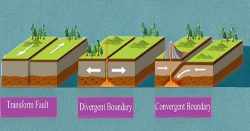
If we imagine the Earth as a jigsaw puzzle made up of these massive plates, movement of these plates as they interact with each other causes earthquakes. Mainly there are three types of interactions of tectonic plates at plate boundaries as given below:

1. Divergent Boundaries: At divergent boundaries, tectonic plates move away from each other, letting magma rise and create new crust. A well-known example is the Mid Atlantic Ridge in the Atlantic Ocean, where this process slowly pushes continents apart.
2. Convergent Boundaries: These happen when two tectonic plates collide head on. A good example is the Indian Plate crashing into the Eurasian Plate, forming the majestic Himalayas. Most big earthquakes in this region occur along thrust faults like the Main Boundary Thrust (MBT), Main Central Thrust (MCT), Main Frontal Thrust (MFT), and the Indus-Tsangpo Suture Zone (ITSZ), all caused by huge forces from this collision.
3. In case of transform fault, plates slide horizontally past each other. When movement along these boundaries gets temporarily stuck, something called “ridge lock” occurs, stress builds up until it suddenly releases as an earthquake. The famous San Andreas Fault in California is a classic example of this kind of boundary^{4, 5}.

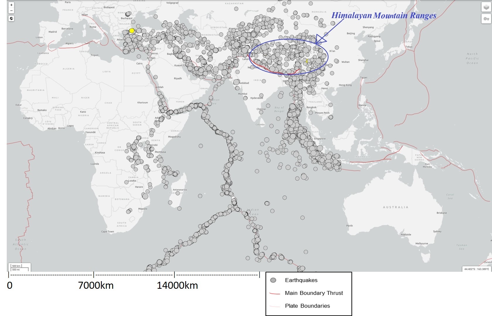
In Figure 2 we can observe that all the earthquakes occur along the plate boundaries. Himalayan mountain ranges are also marked in above figure. Highlighted red marking is Main Boundary Thrust (MBT) of Himalayas, MCT and MFT are not marked but they occur north of MBT.

As discussed in above section, earthquakes happen mainly due to the movement of tectonic plates. These plates meet at plate boundaries and interact as divergent, convergent or transform fault. Due to this interaction stress builds up along these faults. When the stress becomes very high, it is released as an earthquake.

Now as we have a better grasp of what causes earthquakes, the next step is using machine learning to predict them. Although accurate forecasting of earthquakes in short term still remains a challenge but we are steadily getting closer. With the huge amount of seismic and earthquake related data now available, and the rise of powerful computing technologies, we can process complex information faster than ever before. As artificial intelligence and machine learning continue to advance, the next major breakthrough in earthquake prediction could be just around the corner^{6, 7}.

This study aims to evaluate whether supervised learning models can forecast earthquake occurrence in the Himalayas and to quantify the model’s performance disparity between small and large seismic events. To operationalize this objective, the prediction task is defined as a binary classification problem in which each precursor window is labeled by the occurrence of an M ≥ 3.5 earthquake within the following 30 days and within a 100-km radius.

Earthquake Precursors

One area that continues to show substantial potential for advancing earthquake forecasting is the systematic study of earthquake precursors that may precede major seismic events. As documented across various studies and historical records, potential precursors include unusual seismic activity patterns, radon gas emissions, fluctuations in groundwater levels, variations in electric and magnetic fields, surface temperature anomalies, and ground deformation. In certain cases, these geophysical observations have also been supported by reports of abnormal animal behavior, offering an additional insight though less consistent^{1, 8, 9}. However, despite the importance of these observations, most discoveries so far have been coincidental rather than the outcome of planned, predictive monitoring efforts. A notable example of coincidental discovery is the 1989 Loma Prieta earthquake in California, where a magnetometer was initially installed to monitor electromagnetic noise from electric trains and it detected two distinct magnetic anomalies before the main shock. Interestingly, the device was positioned just 7 kilometers from the epicenter of that earthquake. The first signal appeared around two weeks before the earthquake, and the second about three hours prior to earthquake. This event shows the promise of relying on precursor signals for short term earthquake prediction ^{1, 10}.

Given the complication and vastness of precursor data, traditional methods of analysis have got limited success in capturing the intricate patterns hidden within these data. This is where Artificial Intelligence (AI), and particularly machine learning techniques come in picture, they open new opportunities. By training algorithms on diverse geophysical and environmental datasets, machine learning offers the potential to uncover subtle relationships, enhance prediction accuracy, and move the goal of reliable short-term earthquake forecasting closer to reality.

However it is important to note that despite these advances the literature also reveals significant challenges. Several studies have critically evaluated machine learning models and found that many claimed earthquake precursors did not consistently improve forecasting accuracy beyond baseline models.Their work highlights the difficulties in identifying reliable and generalizable earthquake precursors and cautions against overinterpreting optimistic results. Other studies have similarly reported limited success in forecasting large earthquakes due to their rarity and the complex, nonlinear nature of seismic activity. This body of research underscores the need for cautious interpretation of machine learning results in seismology and motivates our focus on a rigorous evaluation of model performance with respect to class imbalance and precursor selection^{11, 12, 7}.

Analysis of Earthquake Precursors and Their Potential for Prediction:

Examining key earthquake precursors and analyzing them with advanced machine learning tools offers a promising path toward improving the accuracy of short-term earthquake prediction and forecasting.

A. Seismic Activity Patterns

One of the most widely observed precursors to earthquakes is an increase in small tremors, these small tremors are known as foreshocks. While not every major earthquake is preceded by a foreshock, their presence suggests rising stress along fault lines. However, sometimes large earthquakes strike without any early tremors^{1, 13}.

B. Radon Gas Emissions

Radon is a naturally occurring radioactive gas; it often sees a spike in concentration sometimes before earthquakes. Scientists believe that this spike happens due to underground pressure shifts or minor cracks forming along fault zones leading to release of Radon gas. But relying only on radon gas emission for early warnings is not recommended as the signals are mostly very small or too scattered^{1, 8}.

C. Groundwater Level Fluctuations

In numerous cases changes in groundwater levels have been observed before major earthquakes this is most likely due to stress alterations deep underground as a result of tectonic movements. However, groundwater is highly sensitive to many external factors, such as rainfall and human activities. Continuous and careful monitoring is essential to distinguish between changes caused by natural tectonic processes and those resulting from other factors^{1, 8}.

D. Electromagnetic and Magnetic Field Variations

Changes in the Earth’s local magnetic field have often been observed ahead of major earthquakes. A prominent example is the 1989 Loma Prieta earthquake in California, where a magnetometer which was originally installed to monitor noise from nearby trains detected unusual magnetic signals just days before the earthquake. While these findings are promising, magnetic anomalies are not yet consistent or reliable enough to be used as a dependable warning system^{14, 8}.

E. Surface Deformation

It has been observed that sometimes before the start of major earthquake the earth’s surface may slightly rise, sink, or stretch. These small changes are very small to observe on ground but they can be captured using satellite technologies like InSAR (Interferometric Synthetic Aperture Radar)^{1, 15}.

F. Animal Behavior

There are reports of unusual animal behavior such as restless dogs and cats, nervous livestock, or sudden bird migrations before the earthquakes. Scientific proof of occurrence remains limited however these signs still offer some hints into how animals might sense changes in the environment. These behaviors are most commonly observed near the epicentral region, especially during earthquakes with magnitudes greater than 5 on the Richter scale^{14, 8}.

G. Vp/Vs ratio

Early investigations in the 1970s proposed that changes in the Vp/Vs ratio was driven by stress induced microcracking and it might serve as an earthquake precursor. However, subsequent assessments by the USGS and independent researchers found that such anomalies were inconsistent, difficult to reproduce, and not dependable for forecasting¹⁶.

In this study, Vp/Vs was not included as a precursor feature because the USGS earthquake catalog does not provide Vp/Vs data .

The Role of Machine Learning in Earthquake Forecasting

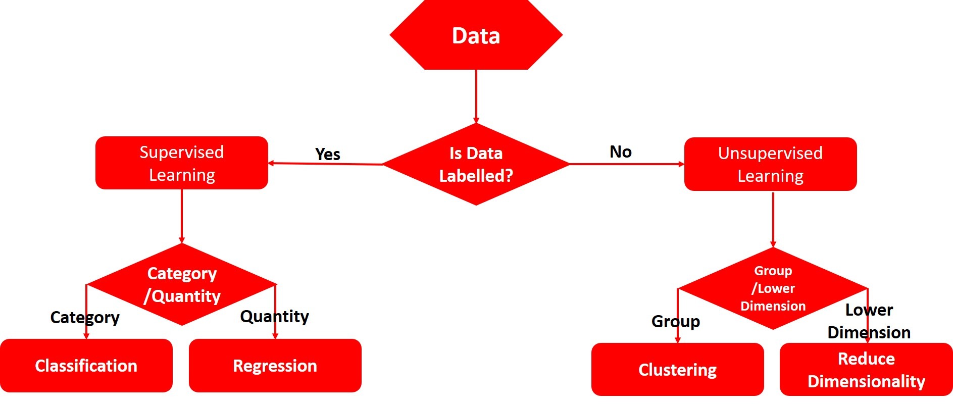
Humans can’t prevent natural disasters like earthquakes as they occur at the level of tectonic plate movements. However, we can leverage Machine Learning (ML) to uncover hidden patterns in data. This can significantly enhance our ability to predict such events.ML techniques are typically divided into two main types: Supervised Learning (SL) in which the model is trained on labeled data and Unsupervised Learning (UL) where the model identifies patterns in data without the need for predefined labels.

As shown in the Figure 3 Supervised Learning uses the model which is trained using labeled data meaning each input comes with a known output. Supervised Learning algorithm can result into two main types of predictive models, which are  1. regression model for forecasting numerical values and 2. classification model for classifying data into different groups. This approach helps the model understand and make proper predictions on the basis of an known relationships in the data Unsupervised Learning works with unlabeled data, in this case structure uses its own intelligence to detect hidden patterns, relationships and clusters within the data. Unsupervised Learning tries to group the data based on similarities and differences.

It is well known fact that no single machine learning algorithm performs optimally across all datasets and conditions. The performance of any algorithm can vary depending on factors like the size of the dataset, the type of input data, and the overall complexity of the problem. Some algorithms work on small datasets better, while others work on larger ones in better way. Also, certain models are designed to handle quantitative inputs, whereas other models are more compatible with qualitative dataset. We must consider the complexity of the dataset and the number of features that the model must learn before selecting appropriate algorithm^{17, 18}

Dataset description

The earthquake catalog was obtained from the United States Geological Survey (USGS) for the Himalayan region (22nd april 2000–22nd april 2025). The dataset includes the event origin time, latitude, longitude, depth, and magnitude (mag) along with the corresponding magnitude type (magType). Additional quality and network metadata provided in the catalog included the number of seismic stations used (nst), azimuthal gap (gap), closest station distance (dmin), root-mean-square travel-time residuals (rms), and the reporting network code (net). The dataset also contains administrative identifiers such as the event ID, update timestamp, location description (place), and event type (e.g., earthquake, quarry blast). Measurement uncertainties are provided as horizontal error, depth error, and mag error, along with the number of stations contributing to the magnitude estimate (magNst). A concise summary is shown in Table:1.

Parameter	Description / Value
Data Source	USGS (United States Geological Survey)
Time Period Covered	April 2000 to April 2025
Geographic Region	Himalayas (the latitude  26.125°–39.676° and longitude  67.4179°–97.6714°)
Total Number of Events	12910
Magnitude Range (Mw)	>3.5
Completeness Magnitude (Mc)	~3.0
Number of Small Events (M Between 3.5 to 5)	11966 (92.69%)
Number of Large Events (M ≥ 5)	944 (7.31%)
Declustering Method	Gardner–Knopoff windowing
Dependent Events Removed	~22%
Events Used After Declustering	10055
Features Used	Time, latitude, longitude, depth, magnitude
Aftershock Treatment	Aftershocks removed; mainshocks retained
Data Format	Raw CSV from USGS

Methodology

In this study we focused on earthquake data from the Himalayan mountain belt which is one of the most seismically active regions in the Indian subcontinent. Given the high frequency of earthquakes in this area, the Himalayas provided an ideal case for earthquake forecasting study. All the data was sourced from the United States Geological Survey (USGS) (website: https://earthquake.usgs.gov.)

To support the development of the forecasting model, a comprehensive set of precursor features were derived from the USGS earthquake catalog. These features include seismicity metrics, statistical descriptors, and physical estimators commonly used in earthquake prediction research.

Feature Definition	Definition	Sampling	Frequency	Preprocessing	Steps
b-value	Slope of Gutenberg-Richter relation indicating stress state	USGS	Unitless	30 days rolling window	Magnitude filtering , linear regression
a-value	Seismic productivity parameter from Gutenberg-Richter relationship	USGS	Unitless	30 days rolling window	Derived from Gutenberg-Richter fit
Seismicity rate	Number of events in a given period	USGS	Count	30 days	Event counting
Cumulative Seismic moment	Total strain energy released	USGS	Newton-meters	30 days rolling window	Converted from magnitude
Inter-Event time	Time between consecutive events	USGS	Seconds	Event-based	Time differencing
Inter-Event distance	Spatial distance between consecutive event	USGS	Km	Event-based	Haversine calculation
Depth variability	Standard deviation of event depths	USGS	Km	30 days	Statistical computation
magnitude Variability	Standard deviation of magnitude	USGS	Unitless	30 days rolling window	Statistical computation
Energy Release rate	Energy per unit time	USGS	Joules/day	30 days rolling window	Energy conversion and averaging

Table 2 provides a detailed overview of all precursor features used in this study which were derived from raw USGS data, including their definitions, data sources, units, sampling frequency, and preprocessing steps.

All precursor features used in this study are derived exclusively from parameters available in the USGS earthquake catalog, including magnitude, event time, latitude, longitude, depth etc. Following features were calculated over defined spatial window of 100km  and temporal windows of 30 days to capture relevant seismic patterns.

Gutenberg-Richter relationship is defined by the emperical equation log₁₀N = a − bM

Where:

N = number of earthquakes with magnitude ≥ Mmin

a-value = seismic activity level (intercept)

b-value= relative proportion of small to large earthquakes (slope)

M = magnitude⁴

b-value: Derived from the Gutenberg–Richter relationship, quantifies the relative frequency of small versus large earthquakes and reflects the regional stress state. It was obtained by fitting a linear regression to the log-transformed frequency magnitude distribution within a one month rolling window and 100 km spatial radius .

a-value: Represents seismic productivity and corresponds to the intercept of the Gutenberg–Richter regression line .

Seismicity rate: Measures the number of earthquake events within a specified time interval (daily, weekly, or monthly), indicating variations in seismic activity .

Cumulative seismic moment: Quantifies the total strain energy released and is calculated by converting magnitudes to seismic moments using the formula M₀=10^{1.5M + 9.1}​ and summing over the analysis window .

Inter-event time:  Defined as the time interval between successive earthquakes, computed by differencing event timestamps.

Inter-event distance:Measures the geographic separation between consecutive earthquake epicenters using the Haversine formula applied to their latitude and longitude.

Depth variability and Magnitude variability :Standard deviations of event depths and magnitudes, respectively, within the analysis window, reflecting spatial and size heterogeneity in seismicity .

Energy release rate :Estimates the average seismic energy released per unit time by converting magnitudes to energy via E=10^1.5M+4.8 and averaging over the time window⁴.

Collectively, these features capture essential aspects of seismicity and provide a robust basis for earthquake forecasting using USGS catalog data alone.

Precursors such as radon gas emission, Vp/Vs ratio, electromagnetic fields, animal behavior and groundwater fluctuations were not used in this study due to the absence of corresponding data in the USGS earthquake catalog and limited availability of consistent and reliable measurements.

To address the severe class imbalance inherent in earthquake forecasting, particularly due to the rarity of large events, three methodological steps were implemented as follow:

1. Random oversampling was applied to the minority class (defined by windows containing an M ≥ 5event within 30 days and 100 km) to increase its representation in the training set while preserving the temporal order of events. SMOTE was not used, as generating synthetic samples in a time dependent seismic sequence may introduce physically unrealistic patterns.
2. Models that support weighted loss functions were configured with higher penalties for misclassification of the minority class, ensuring that the learning process remains sensitive to large events detection rather than defaulting to the majority which are mainly small events.
3. Evaluation was performed using imbalance aware metrics specifically precision, recall and F1-score for the minority class rather than overall accuracy.

To study and classify the data from USGS site we used Weka 3.8 software and worked on windows operating system. Weka is a widely used open source machine learning software developed in Java. It is an open-source software developed by the University of Waikato, New Zealand. Weka is a powerful tool that supports tasks like data preprocessing, classification, clustering, regression, and visualization. In this study Weka was used to train and evaluate a machine learning model for classifying earthquake events. The model’s performance was measured using several key metrics, including precision, recall, accuracy, F1-score, Matthews Correlation Coefficient (MCC), and the confusion matrix.

Weka software is freely available and maintained under the GNU General Public License. You can find it here: https://ml.cms.waikato.ac.nz/

In this study we worked with a variety of supervised learning algorithms to train and test earthquake predictability. Since earthquake foreshock data is a labeled data so we did not used any unsupervised learning algorithm. Following algorithm were tested:

A. Bayesian Network (also known as Bayes Net or Bayes network)

A Bayesian Network is a type of machine learning algorithm which uses a probabilistic graphical model to understand how different variables are related. we can take it as a map that shows the connections between different pieces of information and how they affect each other. It is useful for forecasting by estimating the likelihood of different possibilities. This approach is useful in situations where there is high data uncertainty like earthquake forecasting. Although it takes a bit longer to train the data as it carefully studies the underlying relationships between variables before making any predictions^17,19.

To better understand Bayesian Network let’s assume if there have been frequent small earthquakes and the tectonic plates are moving faster than usual near the subduction zone. The Bayesian network will combine these two clues to estimate the chance of a major earthquake. Beauty of this method is that it works if some data is missing or incomplete.

B. Random Forest

Random Forest is a supervised machine learning method. Instead of relying on just one decision tree random forest builds many decision trees. Each decision tress is trained on different pieces of the data. To make the prediction, it asks each decision tree for prediction like whether an earthquake will occur or not. It asks all the trees to provide their answers and goes with the majority vote.

Decision tree model is more accurate and less likely to be impacted by poor data.

C. Random Tree

A Random Tree is a type of machine learning algorithm closely related to the traditional decision tree but with a twist. It introduces randomness during the learning process. Rather than considering all available features when deciding how to split the data, it randomly selects a subset of features at each decision point. This randomness not only speeds up the model’s training but also helps create a more diverse set of trees when used in ensembles like Random Forests. By injecting this element of chance, Random Trees often achieve better accuracy and generalize well, especially when working with complex or noisy datasets.

D. Logistic Model Tree (LMT)

The Logistic Model Tree (LMT) combines decision trees and logistic regression. Imagine a decision tree in which instead of just making a final prediction at the leaves each leaf uses logistic regression to estimate the probability of different outcomes. This hybrid approach makes LMT good at handling complicated data patterns. 

E. Simple Logistic Regression

Simple logistic regression is similar to linear regression, however instead of predicting a number, it predicts categories like “earthquake” or “no earthquake.” Simple logistic regression is useful when your answer needed falls into distinct group rather than continuous values. The main idea here is to calculate the probability of an event happening based on one input. For example, Simple logistic regression could estimate possibility of earthquake based on a specific measurement.

F. ZeroR

ZeroR is the simplest machine learning algorithm available. It completely ignores the input features and bases its predictions solely on the most frequent class in the dataset. For example, if 70% of the data belongs to category A, ZeroR will always predict category A regardless of any other information. While ZeroR does not offer meaningful predictions on its own, it serves an important purpose as a baseline. By comparing more complex models against ZeroR, we can better understand whether those models are actually learning useful patterns or just over fitting noise. We can think of ZeroR as the “null hypothesis” in machine learning which is a simple benchmark to beat^{17, 18}.

Result & Discussion

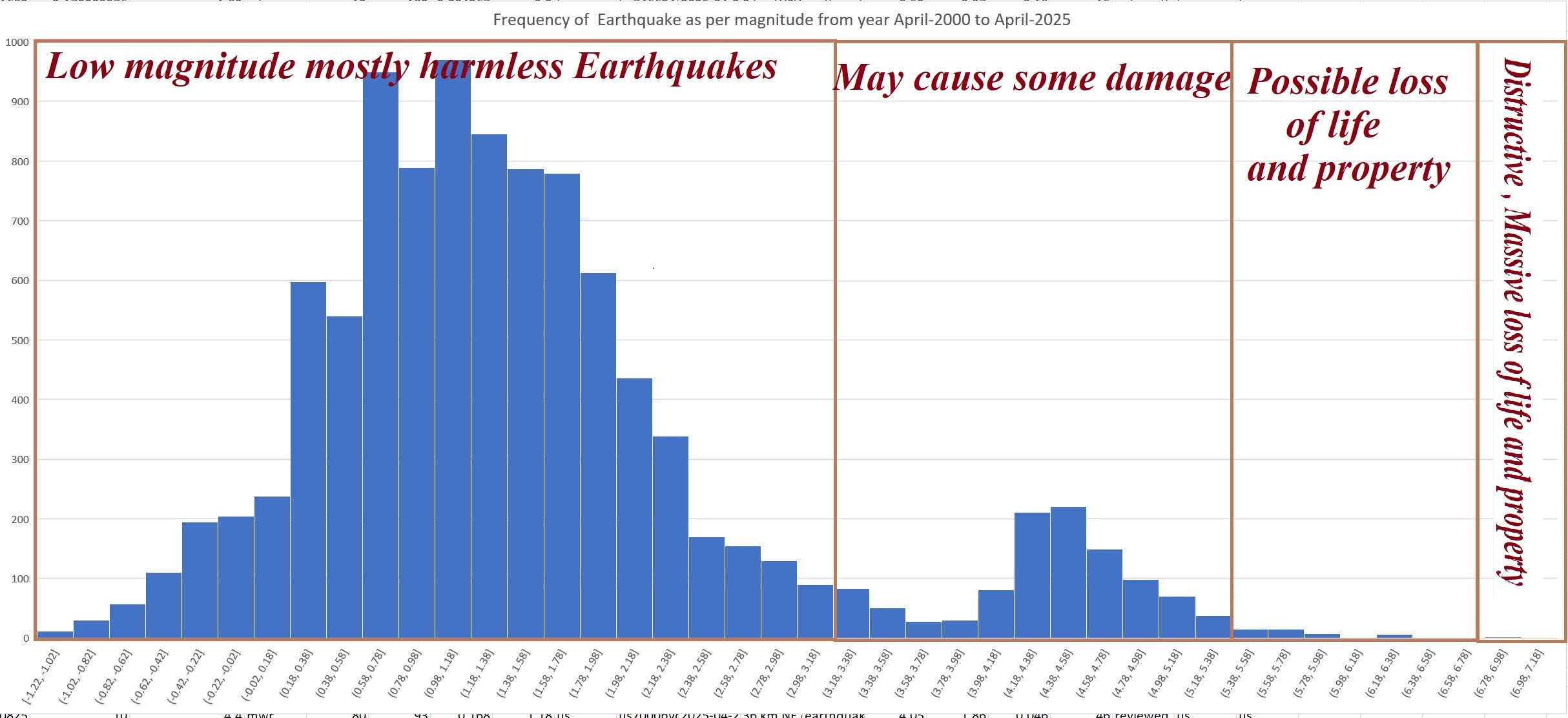
All the algorithms mentioned above were tested on earthquake from the past 25 years, obtained from the USGS website. The analysis was based on the available precursor information discussed earlier. The results showed that smaller earthquakes were easier to predict with better short-term accuracy because they occur more frequently, providing more data for the models to learn from. However, predicting large high magnitude earthquakes was much more challenging, and short term accuracy remained quite low. In fact, across all the algorithms, the ability to accurately forecast the Figure4: Frequency of earthquakes as per their magnitude from Apr-2000 to Apr-2025

biggest and most destructive earthquakes in the short term was very limited. Over the long term, predictions for larger earthquakes were somewhat better, as they mostly rely on recognizing broader patterns of seismic activity over decades. However, long term predictions are generally more useful for identifying where an earthquake might occur, rather than when it will happen.

To evaluate the performance of all the algorithms discussed in previous section, following factors were considered:

1.  Accuracy: Accuracy tells us how often the model makes the right prediction.

2.  Precision : Precision is measure of correct positive predictions.

3.  Recall (Sensitivity): Recall is amount of the actual positive events the model correctly identified.

4.  F1-score: Harmonic mean of precision and recall, providing a single metric that balances both false positives and false negatives. It ranges from 0 to 1, where 1 indicates perfect precision and recall, making it especially useful for evaluating models on imbalanced datasets.

5.  Matthews Correlation Coefficient (MCC): It is a measure of how good the overall classification is.

6. Kappa Statistic: Kappa Statistic tells us how much the model’s predictions match the actual outcomes. A perfect model would get a kappa of 1, while a value of 0 would mean it’s just guessing^17,18.

The results from testing various machine learning algorithms on earthquake data showed that most models performed very well in predicting smaller earthquakes. Algorithms like Bayes Net, Simple Logistic, and Random Tree reported approximately 98% for small-magnitude events.which clearly indicated they were highly reliable in making predictions for smaller and high frequency earthquake. Random Forest and Logistic Model Tree also showed strong performance, with accuracy of above 94 to 95% , proving to be effective for this type of data. Logistic Regression, while slightly behind the top models, still delivered good results with over 91% accuracy. On the other hand, ZeroR, the simplest model that always predicts the majority class, had very low precision and accuracy about 49% even for small earthquake, and although its recall was 100% since it consistently guessed the most frequent outcome. Overall the more advanced algorithms were clearly better at capturing the patterns in the data and making accurate predictions particularly for the small & frequent earthquakes, while the simpler models fell short. Performance metrics of machine learning algorithms for forecasting small, frequent earthquakes are presented in Table 3

Algorithm	Accuracy	Precision	Recall	F1-Score	MCC	Kappa
Bayes Net	0.98	0.97	0.98	0.96	0.96	0.95
Simple Logistic	0.98	0.96	0.97	0.97	0.95	0.94
Random Tree	0.98	0.96	0.98	0.97	0.95	0.94
Random Forest	0.95	0.93	0.95	0.94	0.89	0.88
Logistic Model Tree	0.94	0.92	0.94	0.93	0.87	0.86
Logistic Regression	0.91	0.89	0.9	0.89	0.82	0.81
ZeroR	0.49	0	1	0	0	0

Although the models demonstrate high overall accuracy, it is important to note that accuracy can be misleading in the context of significant class imbalance. Accuracy largely reflects the correct classification of the majority class which in our case are small earthquakes. To address this limitation, we focused on precision, recall, and F1-score metrics specifically for the large earthquakes with M>5. These metrics provide a more meaningful assessment of the model’s ability to detect rare but critical seismic events. Although the reported accuracy highlights strong performance for frequent small earthquakes, the minority class metrics ensure a balanced evaluation of predictive capability across earthquake magnitudes.

Comparison against standard seismology forecasting techniques

In order to place this study in a broader scientific context, it is important to compare the machine learning approach used here with established forecasting frameworks widely adopted in statistical seismology. Models such as the Epidemic Type Aftershock Sequence (ETAS) for decades have provided the most robust representation of clustered seismicity by explicitly modeling aftershock triggering, background seismicity rates and temporal decay laws. ETAS based methods are particularly effective at capturing the cascading nature of earthquake sequences which  general machine learning models, when trained on catalog data alone inherently struggle to reproduce.

Further physics based methods such as Coulomb stress change models offer valuable insight into fault interactions and stress redistribution following large events. These models help quantify how slip on one fault may promote or inhibit failure on neighboring structures resulting into explanations grounded in physical processes rather than purely statistical correlations. Traditional declustering techniques which attempt to separate background seismicity from aftershock sequences  also form an integral part of current operational forecasting methods. Together  these approaches represent mature and thoroughly tested methodologies that remain central to seismic hazard estimation^{15, 7, 20}.

Our machine learning results should therefore be interpreted as complementary rather than competitive with these established frameworks. While Bayes Net can identify useful statistical patterns within seismic parameters, they do not inherently model earthquake triggering physics or long term stress evolution. A direct comparison with ETAS forecasts or Coulomb based stress metrics would require additional data, a fundamentally different experimental design, and specialized modeling methods. Nonetheless, the promising classification results shown here provide motivation for future hybrid approaches that integrate the strengths of both machine learning and physics based seismological models

 Limitations

This study has several important limitations that should be acknowledged. First, the feature set used for forecasting is limited exclusively to seismic parameters extracted from the USGS earthquake catalog which resulted into omission of potentially informative geophysical, geochemical, and environmental precursors such as radon emissions, electromagnetic signals, and ground water fluctuations. Second, the forecasting task was defined simply as a binary classification of earthquake occurrence within fixed spatial and temporal windows, which may not fully capture the complexity of seismic processes or the continuous nature of earthquake risk. Lastly, while models demonstrated strong predictive performance for frequent small earthquakes but generalizing these results to rare large magnitude earthquakes remains challenging due to their scarcity and differing underlying mechanisms. Future research should consider integrating more diverse data sources and refining forecasting targets to enhance predictive capabilities.

Recommendations and Way Forward

All Supervised learning models with the exception of ZeroR work quite well when it comes to detecting or forecasting small earthquakes which is an encouraging start. However, we have observed that its performance drops noticeably when applied to large earthquakes and those are the ones that cause the most damage to life and property. This is a critical gap because ultimately, we need to improve early warning system for large and destructive earthquakes to bring the real world benefit of applying machine learning for earthquake forecasting.

Moving forward we need to focus on strengthening the model’s ability to handle large earthquakes. This could mean bringing in more diverse and high- quality data such as incorporating GPS displacement data, satellite observations¹⁵ or early tremor signals that may better capture the early stages of big earthquakes. It may also help to combine machine learning models with geophysics based approaches so that system did not just learning from past patterns but also grounded in the underlying mechanics of earthquakes.

We should also work on regional customization. Since geological conditions vary widely across regions fine tuning the model for specific seismic zones may improve accuracy for large events. Finally working closely with seismologists, data scientists, and disaster response teams will help nsure the research translates into practical and actionable tools.

To summarize, although short term forecasting of small earthquakes is possible but the next big leap will come from improving large earthquake predictions in short term.

Author would also like to highlight that that the current dataset and scope do not allow firm claims about early warning or risk reduction; rather these results should be viewed as preliminary indicators that require further validation.

Acknowledgements

I am deeply grateful to Mr. Tanmoy Dutta, a geologist of International standing and alumnus of the Department of Geology, Indian Institute of Technology, Roorkee. This work would not have been possible without his thoughtful guidance, critical insights and unwavering encouragement throughout the project and during the preparation of this manuscript. I also sincerely thank my teachers and Delhi World Public School for their support and inspiration.

References

1. R. D. Cicerone, J. E. Ebel, and J. Britton, “A systematic compilation of earthquake precursors,” Tectonophysics, vol. 476, no. 1–2, pp. 1–26, 2009 [↩] [↩] [↩] [↩] [↩] [↩] [↩]
2. U.S. Geological Survey, Earthquake Prediction: An Opportunity to Avert Disaster, Washington, DC, USA: U.S. Government Printing Office, 1976 [↩]
3. R. E. Wallace, Northridge Earthquake: An Assessment of Precursory Research, Reston, VA, USA: U.S. Geological Survey, 1996 [↩]
4. W. Lowrie and A. Fichtner, Fundamentals of Geophysics, Cambridge, England: Cambridge University Press [↩] [↩] [↩]
5. S. N. Namowitz, Earth Science, Lexington, MA, USA: D. C. Heath and Company, 1989 [↩]
6. M. H. Al Banna, K. A. Taher, M. S. Kaiser, M. Mahmud, M. S. Rahman, A. S. M. S. Hosen, and G. H. Cho, “Application of Artificial Intelligence in Predicting Earthquakes: State-of-the-Art and Future Challenges,” IEEE Access, vol. 8, pp. 22039–22056, 2020 [↩]
7. P. G. Okeke and J. V. D. Spiegel, “A review of data-driven approaches for earthquake forecasting,” Earth-Science Reviews, vol. 208, p. 103266, 2020 [↩] [↩] [↩]
8. S. Van Der Meijde et al., “Geophysical and geochemical signatures associated with earthquake precursors: A review,” Tectonophysics, vol. 744, pp. 34–54, Jul. 2018 [↩] [↩] [↩] [↩] [↩]
9. U.S. Geological Survey, Earthquake Prediction: An Opportunity to Avert Disaster. Washington, DC, USA: U.S. Government Printing Office, 1976 [↩]
10. R. E. Wallace, Northridge Earthquake: An Assessment of Precursory Research. Reston, VA, USA: U.S. Geological Survey, 1996 [↩]
11. A. Mignan and M. Broccardo, “Neural network applications in earthquake prediction (1994–2019): Meta-analytic and statistical insights on their limitations,” Seismological Research Letters, vol. 91, no. 4, pp. 2330–2342, 2020 [↩]
12. J. Zhuang et al., “Machine learning applications for earthquake early warning,” Seismological Research Letters, vol. 91, no. 2A, pp. 715–727, Mar. 2020 [↩]
13. K. M. Khattri and A. K. Tyagi, “Seismicity patterns in the Himalayan plate boundary and identification of the areas of high seismic potential,” Tectonophysics, vol. 96, no. 3–4, pp. 281–297, 1983 [↩]
14. R. D. Cicerone, J. E. Ebel, and J. Britton, “A systematic compilation of earthquake precursors,” Tectonophysics, vol. 476, no. 1–2, pp. 1–26, Oct. 2009 [↩] [↩]
15. G. Cremen and C. Galasso, “Earthquake early warning: Recent advances and perspectives,” Earth-Science Reviews, vol. 205, p. 103184, 2020 [↩] [↩] [↩]
16. United States Geological Survey,”Earthquake Hazards Program,” USGS [↩]
17. K. P. Murphy, Probabilistic Machine Learning: An Introduction. Cambridge, MA, USA: MIT Press, 2022 [↩] [↩] [↩] [↩]
18. S. Raschka, Y. Liu, and V. Mirjalili, Machine Learning with PyTorch and Scikit-Learn: Develop Machine Learning and Deep Learning Models with Python. Birmingham, UK: Packt Publishing, 2022 [↩] [↩] [↩]
19. M. Hutter, Universal Artificial Intelligence: Sequential Decisions Based on Algorithmic Probability, 2nd ed. Cham, Switzerland: Springer, 2021 [↩]
20. Y. Ogata, “Statistical models for earthquake occurrences and residual analysis for point processes,” Journal of the American Statistical Association, vol. 83, no. 401, pp. 9–27, 1988. [↩]