
Abstract
The Hasse–Minkowski Theorem is a central result in number theory that connects local and global perspectives on quadratic equations. It states that a quadratic equation with rational coefficients has a non-trivial rational solution if and only if it has a solution over the real numbers and over every  -adic field. This idea shows how studying equations locally, one prime at a time, can determine whether they have a global solution. This paper offers an expository overview of the theorem and its mathematical foundation. It begins with quadratic forms and their properties, such as discriminants and isotropy, then introduces local fields and -adic numbers, which describe completions of
  . The discussion highlights the Hilbert symbol and the Hilbert Reciprocity Law, which connect local conditions to produce the global result established by the theorem. Several examples and applications are explored, including the representation of integers as sums of squares and the classification of rational solutions. The paper concludes by showing how the local–global principle underlying this theorem continues to shape modern number theory, linking classical results with ongoing research in arithmetic geometry and algebraic structures.
Keywords: Hasse–Minkowski theorem, quadratic forms, -adic numbers, Hilbert symbol, local–global principle, number theory
Introduction
The Hasse–Minkowski Theorem is a cornerstone in the theory of quadratic forms over number fields, offering a powerful local-global principle. It addresses the question of whether a quadratic equation, such as  , has a non-trivial solution (i.e. not all variables are zero) in rational numbers by checking its solvability in the real numbers and the -adic numbers, which are completions of the rationals with respect to prime-based metrics1. Similarly, it determines when two quadratic forms are equivalent, meaning one can be transformed into the other via a linear change of variables. Historically, Hermann Minkowski proved the theorem for rational numbers, and Helmut Hasse generalized it to number fields. Its significance lies in its use of -adic numbers, introduced by Kurt Hensel, to solve arithmetic problems, marking a significant advancement in number theory. This paper focuses on the theorem over , providing a clear exposition suitable for readers familiar with introductory algebra and number theory. The Hasse–Minkowski Theorem emerged from Hermann Minkowski’s work on quadratic forms in the early 20th century, building on Kurt Hensel’s discovery of -adic numbers in 1897. Helmut Hasse later generalized it to number fields, formalizing the local-global principle. This theorem revolutionized number theory by providing a systematic method for solving Diophantine equations using local fields, thereby establishing it as a cornerstone for modern algebraic geometry and arithmetic. Consider the equation
![\[x^{2}+y^{2}=3z^{2}.\]](https://nhsjs.com/wp-content/ql-cache/quicklatex.com-45894a930592b987f217f42940a1865b_l3.png "Rendered by QuickLaTeX.com")
Does it admit a non-trivial rational solution? Over  the form is indefinite, so solutions certainly exist, e.g.
  . Over
  , we can check for solutions by assuming
  and are not all divisible by 3 (by scaling). The equation
  modulo 3 becomes
  . Since the quadratic residues mod 3 are 0 and 1, this requires
  and
and  . This means
  and
and  are divisible by 9. So
  , which simplifies to
  . This implies
  must also be divisible by 3. Since
  and are all divisible by 3, this contradicts our assumption. Therefore, the only solution in is the trivial one
  .
.
Since a local obstruction appears at  , there can be no rational solution. This illustrates the “easy” direction of Hasse–Minkowski: any rational solution must survive in every completion, so a failure in blocks global solvability. The deep content of the Hasse–Minkowski Theorem is the converse: if a quadratic form has a non-trivial solution over and every
  , then it necessarily has one over . This local-global principle is special to quadratic forms; for higher-degree equations (such as Selmer’s cubic) local solvability does not imply global solvability.
Preliminaries and Definitions
Throughout,  denotes a field of characteristic
  . Boldface letters
  ,
,  represent column vectors.
Quadratic Forms
Definition 1 (Quadratic Form): Let  . A quadratic form in
  variables over is a homogeneous polynomial of degree 2,
![\[Q(x_1,\dots,x_n) =\sum_{i\le j}c_{ij}x_ix_j =(x_1 x_2 \cdots x_n) A \begin{pmatrix}x_1 x_2 \vdots x_n\end{pmatrix},\]](https://nhsjs.com/wp-content/ql-cache/quicklatex.com-48cb5ab0d74aa0f9916c9fe91bc768b9_l3.png "Rendered by QuickLaTeX.com")
where  is an
is an  symmetric matrix over .
Isotropic vectors and hyperbolic planes
Definition 2 Let  be a quadratic form on an -vector space
  and
and  .
.
• is isotropic (for ) if  .
.
• (or ) is isotropic if it possesses an isotropic vector; otherwise it is anisotropic.
Definition 3 (Bracket notation for diagonal forms): If  , we write
![\[\langle a_{1},\dots,a_{n}\rangle\]](https://nhsjs.com/wp-content/ql-cache/quicklatex.com-4d8a9cfcfe19fd6cf466a7f2c7a9f10c_l3.png "Rendered by QuickLaTeX.com")
for the diagonal quadratic form  . Thus, for instance,
  denotes the hyperbolic plane
  .
.
Definition 4 (Hyperbolic plane): The binary form  is called the hyperbolic plane. Equivalently,
  . It contains the isotropic vectors
  and
and  , which are linearly independent.
Remark 1 Any two-dimensional isotropic subspace of a non-degenerate quadratic space over is -isometric to  . Hyperbolic planes will be the “building blocks” in Witt decomposition.
Example 1 (Isotropic vs. anisotropic): Over the form  is isotropic because
  . In contrast,
  is anisotropic over (both terms are
  and vanish simultaneously only at
  ).
).
This distinction has a geometric interpretation as shown in Figure 1, which depicts an indefinite quadratic form whose zero set is non-trivial. The surface intersects the plane  along a cone, corresponding to non-zero vectors for which the quadratic form vanishes.
Over the situation reverses:  becomes isotropic because reducing the equation
  modulo
  gives
gives
![\[x^2+2y^2 \equiv x^2-y^2 \equiv 0 \pmod{3},\]](https://nhsjs.com/wp-content/ql-cache/quicklatex.com-3fa6c5f5a42384c0798726729478e63e_l3.png "Rendered by QuickLaTeX.com")
since  . This congruence has non-trivial solutions, for example

whereas  is anisotropic.
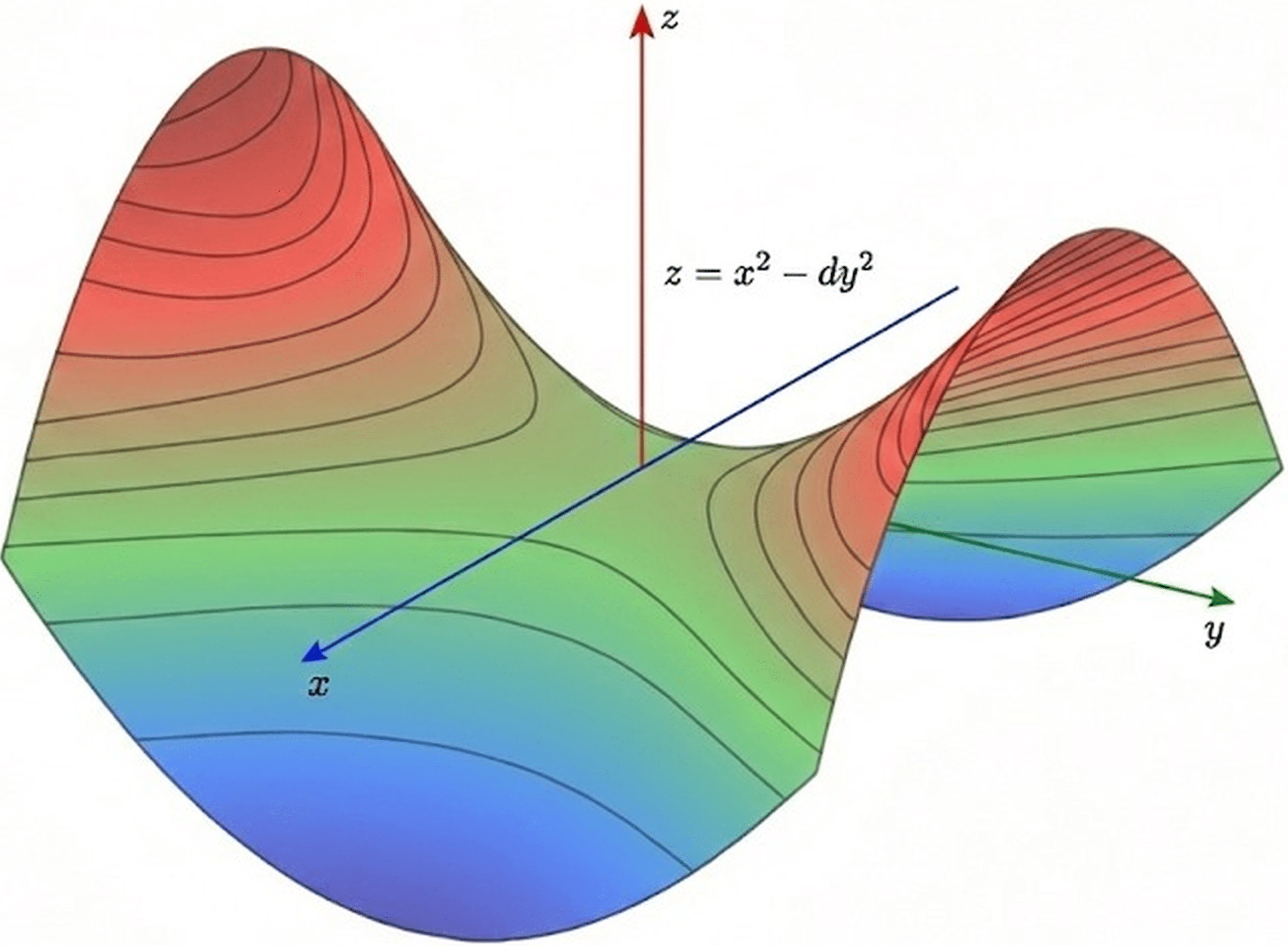
 for
for  , an example of an indefinite quadratic form. Its zero set is a double cone, illustrating the geometric origin of isotropic vectors.
Definition 5 (Equivalence): Quadratic forms  in variables over are equivalent over if some
  (the group of invertible matrices over ) satisfies
  for every
  .
.
Proposition 1 Every non-degenerate quadratic form over is equivalent to a diagonal form
![\[Q(x_1,\dots,x_n)=a_1x_1^2+\dots+a_rx_r^2, a_i\in F^\times,\]](https://nhsjs.com/wp-content/ql-cache/quicklatex.com-273d5b2201793581f057d0e48c41c980_l3.png "Rendered by QuickLaTeX.com")
where  (see Definition 6).
Sketch. Write  with
with  symmetric. Since
  , the element
  is invertible in , which allows us to complete the square. If a diagonal coefficient
  , then all terms involving
  can be grouped and rewritten by completing the square. After a suitable linear change of variables, this eliminates all cross terms involving , leaving a single squared term together with a quadratic form in one fewer variable. Repeating this process inductively removes all off-diagonal terms and yields a diagonal form2.
Example 2 (Diagonalising a binary form over ): Consider the form
![\[Q(x,y)=3x^{2}+4xy+5y^{2}.\]](https://nhsjs.com/wp-content/ql-cache/quicklatex.com-6b4747b3340bb5d95033675880854007_l3.png "Rendered by QuickLaTeX.com")
Its coefficient matrix is  So
So  and is non-degenerate. Completing the square gives
![\[Q(x,y)=3\Bigl(x+\tfrac23y\Bigr)^{2}+\tfrac{11}{3}y^{2}.\]](https://nhsjs.com/wp-content/ql-cache/quicklatex.com-282c31ada4ba40e99a3b4810bde2a9d3_l3.png "Rendered by QuickLaTeX.com")
Writing  (matrix
  ) We obtain the diagonal form
  .
.
Definition 6 (Rank): For , the rank of is  , i.e. the dimension of the largest subspace on which is not identically 0.
Remark 2 After diagonalisation,  is the number of non-zero diagonal coefficients.
Field extensions
Definition 7 (Field extension): An extension  is a pair of fields with
  . Its degree is
 ![[K:F]=\dim_{F}K](https://nhsjs.com/wp-content/ql-cache/quicklatex.com-a276cb8d2948f08ea70b52c7070b32b2_l3.png "Rendered by QuickLaTeX.com") as an -vector space.
as an -vector space.
Definition 8 (Finite & quadratic extensions): An extension is finite if ![[K:F]<\infty](https://nhsjs.com/wp-content/ql-cache/quicklatex.com-e57a18c8fcc20bd55cf8988243b4d0bf_l3.png "Rendered by QuickLaTeX.com") . If
. If ![[K:F]=2](https://nhsjs.com/wp-content/ql-cache/quicklatex.com-36f6443407d907f96c2a124940419657_l3.png "Rendered by QuickLaTeX.com") it is called quadratic. Every quadratic has the form
it is called quadratic. Every quadratic has the form  for some
  .
.
Definition 9 (Separable): For characteristic  (in particular,
  ) every algebraic extension is automatically separable: every element’s minimal polynomial over splits into distinct roots in a splitting field.
Remark 3 Finite separable extensions admit well-defined field trace  and norm
  . These appear later when we relate the Hilbert symbol to norm forms.
Example 3 (Quadratic extension of  ): Set
  . The minimal polynomial of
  over is
  , so
, so ![[K:\mathbb Q]=2](https://nhsjs.com/wp-content/ql-cache/quicklatex.com-7437793de4f09e9df4013b1a87c59e57_l3.png "Rendered by QuickLaTeX.com") ; hence
; hence  is quadratic (and separable). For
 :
:
![\[\operatorname{Tr}_{K/\mathbb Q}(\alpha)=2x, \operatorname{N}_{K/\mathbb Q}(\alpha)=x^2-5y^2,\]](https://nhsjs.com/wp-content/ql-cache/quicklatex.com-d1022071ecfb91a2f01f65d56cd344fd_l3.png "Rendered by QuickLaTeX.com")
The latter gives the Pell conic  .
.
Fields, absolute values, and completions
Definition 10 (Absolute value): An absolute value on a field  is a map
  such that
1.  ;
;
2.  ;
;
3.  .
.
It is non-Archimedean if  .
.
On there are, up to equivalence, exactly the usual absolute value  and the -adic absolute values
  , one for each prime 3.
Definition 11 (Completion): Let  be a valued field. Its completion
  is the metric completion of with respect to
  . We write
![\[\mathbb{Q}_\infty=\mathbb{R}, \mathbb{Q}_p (p\text{ prime})\]](https://nhsjs.com/wp-content/ql-cache/quicklatex.com-f3874b9d389866aa4802e6be26e833e7_l3.png "Rendered by QuickLaTeX.com")
for the completions of .
Example 4 (Real vs. -adic magnitude): Take  . The ordinary absolute value is
  , but factorising
  gives
gives  and
and  . Thus, a “small” real can be “large”
  -adically.
Bilinear forms, discriminant, Witt decomposition
Definition 12 (Discriminant): Let be a non-degenerate quadratic form in variables over , represented by a symmetric matrix . Define
![\[\disc(Q) = (-1)^{n(n-1)/2}\det A \in F^{\times}/F^{\times 2}.\]](https://nhsjs.com/wp-content/ql-cache/quicklatex.com-488b26aa87c15a2374a61eb3e972f19e_l3.png "Rendered by QuickLaTeX.com")
That is, the discriminant is the determinant of , corrected by a sign depending on , taken modulo the subgroup of square elements.
Remark 4 If  and
and  are equivalent quadratic forms over (see Definition 5), then
  in
in  . Indeed, if
  with
with  , then their coefficient matrices satisfy
  , so
, so
![\[\det(A_{2}) = \det(T)^{2} \det(A_{1}).\]](https://nhsjs.com/wp-content/ql-cache/quicklatex.com-e696bd3badffb086aebbd06eefca18f5_l3.png "Rendered by QuickLaTeX.com")
Thus, the two determinants differ by a square in  , and hence represent the same class in .
Every quadratic form yields such a  by
by  .
.
Example 5 For the diagonal ternary form  we have
![\[\disc\bigl(\langle 1,1,1\rangle\bigr) =(-1)^{3}= -1 \text{in } \mathbb{Q}^{\times}/\mathbb{Q}^{\times2}.\]](https://nhsjs.com/wp-content/ql-cache/quicklatex.com-465d121d0c76767f6674d47705345d8d_l3.png "Rendered by QuickLaTeX.com")
Hence  is not -equivalent to
  , whose discriminant is
  .
.
Example 6 (Hyperbolic plane):  is isotropic, since is a non-trivial zero. Any isotropic plane is -isometric to
  .
.
Definition 13 (Orthogonal sum): If and are quadratic forms over , their orthogonal sum is written
![\[Q_{1} \perp Q_{2},\]](https://nhsjs.com/wp-content/ql-cache/quicklatex.com-d17d854b25285316f436264f88a3b107_l3.png "Rendered by QuickLaTeX.com")
and defined on the direct sum of the underlying vector spaces by
![\[(Q_{1} \perp Q_{2})(v_{1},v_{2}) = Q_{1}(v_{1})+Q_{2}(v_{2}).\]](https://nhsjs.com/wp-content/ql-cache/quicklatex.com-955a699be95ae39d2d8c71b7df8df68c_l3.png "Rendered by QuickLaTeX.com")
More generally,  denotes the orthogonal sum of
  copies of .
Theorem 1 (Witt decomposition): Every non-degenerate quadratic form over decomposes uniquely (up to isometry) as
![\[Q \cong \mathbb{H}^{\perp r} \perp Q_{\mathrm{an}},\]](https://nhsjs.com/wp-content/ql-cache/quicklatex.com-a15359ef793df13b737735f085439de0_l3.png "Rendered by QuickLaTeX.com")
where is the hyperbolic plane and  is anisotropic. The integer is the Witt index of . See4.
Example 7 (Witt decomposition of a quaternary form): Let
![\[Q = \langle 1,1,-1,-1\rangle = x^{2} + y^{2} - z^{2} - w^{2}.\]](https://nhsjs.com/wp-content/ql-cache/quicklatex.com-1de8c7c76c8b0acd12e687c8bd1725ad_l3.png "Rendered by QuickLaTeX.com")
Choose isotropic vectors  and
and  with
with  . They span a hyperbolic plane ; repeating with another pair yields
![\[Q \cong \mathbb{H} \perp \mathbb{H},\]](https://nhsjs.com/wp-content/ql-cache/quicklatex.com-49267fd173dcc502c05ba5dca0f5cbd4_l3.png "Rendered by QuickLaTeX.com")
so the Witt index is and the anisotropic part is .
Norms and traces in quadratic extensions
For  and
and  , put
, put
![\[\operatorname{Tr}_{K/F}(\alpha)=2x,\operatorname{N}_{K/F}(\alpha)=x^{2}-dy^{2}.\]](https://nhsjs.com/wp-content/ql-cache/quicklatex.com-79892352fe305daeac5facaaeb390d7f_l3.png "Rendered by QuickLaTeX.com")
The norm form is a basic 2-variable quadratic form whose local isotropy answers norm-related questions.
Local Fields and Completions
Classical Diophantine problems over can often be understood one prime at a time. This idea is made precise by working in the  of —the real field at the infinite place and the -adic fields at each finite place .
Ostrowski’s classification of norms on
Proposition 2 (Product formula): For every  ,
, 
Theorem 2 (Ostrowski, 1916): Every non-trivial absolute value on is equivalent to either
![\[|\cdot|_\infty \text{(the usual Archimedean norm)} \text{or} |\cdot|_p (p \text{ a prime}).\]](https://nhsjs.com/wp-content/ql-cache/quicklatex.com-99a6c160f82c4cfe26e36f9b8a873220_l3.png "Rendered by QuickLaTeX.com")
No other inequivalent norms exist.
Idea of proof. For any  write
write  . If
. If  is non-Archimedean one shows
  for a single prime
  ; rescaling makes it
  . If is Archimedean, Kronecker’s lemma implies it coincides (up to equivalence) with the usual absolute value. A more detailed proof can be found at5.
Remark 5 Ostrowski’s theorem shows that, up to equivalence, the only non-trivial completions of are the real field (corresponding to  ) and the -adic fields for primes . Hence, when we say a statement holds “at every completion of ,” we really mean: it holds over and over for each prime . Verifying local conditions at these places is therefore exhaustive in the Hasse–Minkowski theorem.
Example 8 (Product formula sanity check): For  one has
![\[|30|_\infty = 30, |30|_{2}=2^{-1}, |30|_{3}=3^{-1}, |30|_{5}=5^{-1}, |30|_{p}=1 (p\neq2,3,5).\]](https://nhsjs.com/wp-content/ql-cache/quicklatex.com-d3857ff1a360716d1d9b30996c0db61e_l3.png "Rendered by QuickLaTeX.com")
Hence  , illustrating the global product formula used implicitly in Ostrowski’s proof.
p-adic valuation and norm
Definition 14 (-adic valuation): For a prime and a non-zero rational  , write
  with
with  not divisible by . Set
  and
and  .
.
Definition 15 (-adic norm): The -adic norm is
![\[|x|_{p}=p^{-v_{p}(x)}, x\in\mathbb{Q}.\]](https://nhsjs.com/wp-content/ql-cache/quicklatex.com-b866646b84f5e287f54c3bba643b9f46_l3.png "Rendered by QuickLaTeX.com")
It satisfies the non-Archimedean inequality  .
.
Completions and the field Qp
Completing  in the metric
  yields the -adic field
  . For the usual absolute value, we obtain
  . Elements of can be written as series
  with digits
  .
.
Constructing p-adic Numbers
As mentioned above, the -adic numbers arise as the completion of with respect to the -adic norm. For example, in  , the number
  can be written as a -adic series:
![\[\frac{1}{1-5} = \sum_{n=0}^\infty 5^n = 1 + 5 + 5^2 + \cdots.\]](https://nhsjs.com/wp-content/ql-cache/quicklatex.com-8b86ce652e3bc8351376039a2ead1dbd_l3.png "Rendered by QuickLaTeX.com")
This series converges in because  as
as  . Figure 2 illustrates the hierarchical structure of the -adic integers
  , showing how residue classes modulo higher powers of nest within one another.
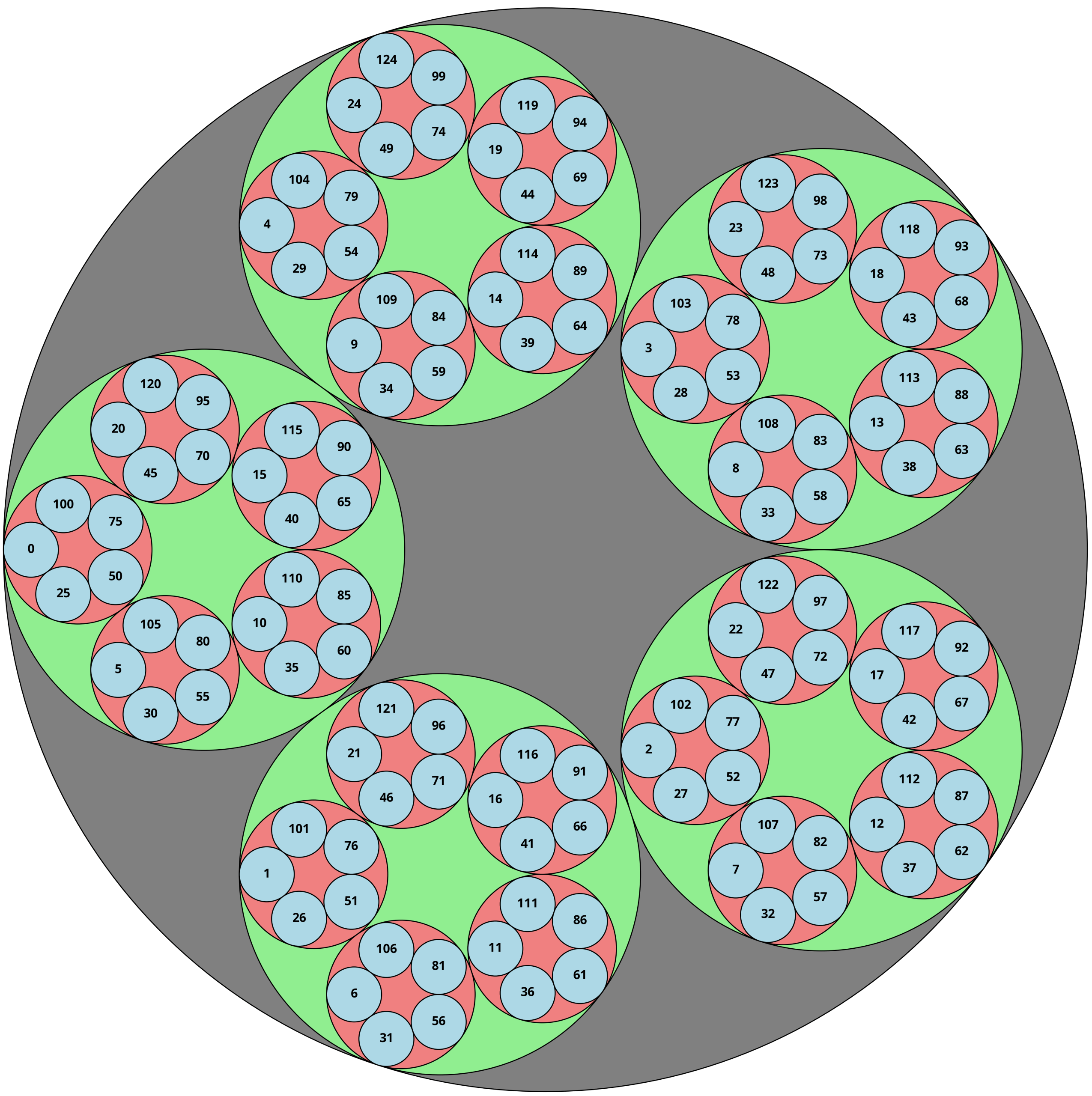 , showing the nested structure of residue classes modulo and their further refinement modulo
  ,
,  , and so on
Figure 3 illustrates how the partial sums converge -adically even though their absolute size grows in the real numbers.
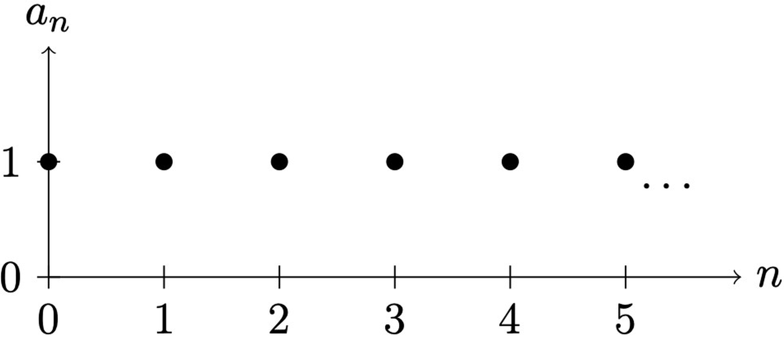 -adic expansion of
  in . Each dot represents
  .
.Such series make a complete field, enabling tools like Hensel’s lemma for solving equations.
Topology of
Each is locally compact (meaning every point has a compact neighborhood) and totally disconnected (meaning the only connected subsets are single points). The compact open unit group  (the -adic integers with no factor of ) is pro-cyclic for
  (it is the limit of cyclic groups).
Strong approximation
The strong approximation theorem states that for any finite set  of primes, the diagonal embedding
  is dense. This means any set of -adic numbers in these fields can be simultaneously approximated by a single rational number. This property is key, as it lets us patch local solutions into a global one once obstructions vanish.
Why bother with completions?
• Analytic control. Limits exist in a completion, so Newton iteration and Hensel’s lemma can lift solutions of congruences to genuine -adic (hence rational) solutions.
• Local–global philosophy. Many arithmetic statements are true over exactly when they hold in every completion; Hasse–Minkowski for quadratic forms is the prime example.
Hensel’s Lemma
Lemma 1 (Hensel’s Lemma, simple form): Let be a prime and ![f(x)\in\mathbb{Z}_{p}[x]](https://nhsjs.com/wp-content/ql-cache/quicklatex.com-31c4068ac1ab51df1eb32c9af641c157_l3.png "Rendered by QuickLaTeX.com") . Assume there exists
. Assume there exists  such that
![\[f(a_{0})\equiv 0 \pmod{p} \text{and} f'(a_{0})\not\equiv 0 \pmod{p}.\]](https://nhsjs.com/wp-content/ql-cache/quicklatex.com-aa5dacee3444fcdcd8322a9a965b97e4_l3.png "Rendered by QuickLaTeX.com")
Then there is a unique  satisfying
![\[f(\tilde{a})=0 \text{and} \tilde{a}\equiv a_{0}\pmod{p}.\]](https://nhsjs.com/wp-content/ql-cache/quicklatex.com-ba3e9f70e83e196904d5eb17363a91bd_l3.png "Rendered by QuickLaTeX.com")
Equivalently, any root modulo with non-vanishing derivative lifts to a unique root in the entire -adic field .
Example: lifting a square root of 2 from F7 to Q7
We illustrate Hensel’s lemma with the congruence  .
.
1. In  ,
,  , so
, so  is a root modulo
  .
.
2. Let  . Because
  , Hensel’s lemma applies.
3. One Newton–Hensel step (working mod  ).
).
![\[x_{1}=x_{0}-\frac{f(x_{0})}{f'(x_{0})} =3-\frac{9-2}{6} =3-\frac{7}{6}.\]](https://nhsjs.com/wp-content/ql-cache/quicklatex.com-376b6c5288ccdec96b7bad0614f2bd6b_l3.png "Rendered by QuickLaTeX.com")
We need  . Since
  , we have
  .
.
Hence
![\[\frac{7}{6}\equiv 7\cdot41=287\equiv42\pmod{49}, \text{so } x_{1}\equiv 3-42\equiv-39\equiv10\pmod{49}.\]](https://nhsjs.com/wp-content/ql-cache/quicklatex.com-14fd4aa14b30dc335b299885b05fb710_l3.png "Rendered by QuickLaTeX.com")
4. Verification.  . Thus
  is a root modulo . Repeating the process (or invoking Hensel directly) yields a unique
  with
with  and
and  .
.
Remark 6: The condition  is essential for Hensel’s lemma: it ensures the lift exists and is unique.
Isotropy over local fields: quick examples
We record three illustrative calculations that foreshadow the local analysis in the Hasse–Minkowski theorem.
Example 9 (A binary form anisotropic over but isotropic over ): Take  .
.
• Over both terms are non-negative and vanish simultaneously only at ; is anisotropic.
• In  we have
  , and
, and  has solutions ,
  . Hensel’s lemma lifts either to a -adic isotropic vector, so is isotropic over
  .
.
Example 10 (Hyperbolic plane everywhere locally): The form is isotropic over (obvious) and over every , since  always has non-trivial solutions.
These computations illustrate that local isotropy can vary wildly with the place  , highlighting the necessity of checking all completions in the Hasse–Minkowski criterion.
Legendre Symbol and Quadratic Residues
Basic definitions
Definition 16 (Quadratic residue modulo ): Let be an odd prime. An integer  is a quadratic residue modulo if the congruence
![\[x^{2} \equiv a \pmod{p}\]](https://nhsjs.com/wp-content/ql-cache/quicklatex.com-8594dbf1868346b1067a38c63f535411_l3.png "Rendered by QuickLaTeX.com")
has a solution  . Otherwise, is a quadratic non-residue.
Definition 17 (Legendre symbol): For an odd prime and any integer , define
![\[\left(\frac{a}{p}\right) = \begin{cases} 0 &\text{if } p \mid a, 1 &\text{if } a \text{ is a quadratic residue }(\bmod p), -1 &\text{if } a \text{ is a quadratic non-residue }(\bmod p). \end{cases}\]](https://nhsjs.com/wp-content/ql-cache/quicklatex.com-ddb88ce909f5b38cb8143def5f9fd4e2_l3.png "Rendered by QuickLaTeX.com")
The map  descends to a group homomorphism
  .
.
Example 11 (Computing a Legendre symbol): Compute  .Because
  is prime,
![\[\Bigl(\tfrac{7}{19}\Bigr) = 7^{ (19-1)/2}\bmod 19 = 7^{ 9}\bmod 19.\]](https://nhsjs.com/wp-content/ql-cache/quicklatex.com-f4f000358449aa5c1bb6bf1361cd2e69_l3.png "Rendered by QuickLaTeX.com")
Fast exponentiation:
![\[7^{2}=49\equiv11, 7^{4}\equiv11^{2}=121\equiv7, 7^{8}\equiv7^{2}=11.\]](https://nhsjs.com/wp-content/ql-cache/quicklatex.com-dc8befb96ea6ca9612563380df88a21c_l3.png "Rendered by QuickLaTeX.com")
Hence  , so
, so  .. Thus is a quadratic residue modulo .
Quadratic Reciprocity
Theorem 3 (Quadratic Reciprocity Law): For distinct odd primes and  ,
,
![\[\left(\frac{q}{p}\right) \left(\frac{p}{q}\right) = (-1)^{\frac{p-1}{2}\cdot\frac{q-1}{2}}.\]](https://nhsjs.com/wp-content/ql-cache/quicklatex.com-5c578f1be28a9429b19da935a61495bf_l3.png "Rendered by QuickLaTeX.com")
Equivalently,
![\[\left(\frac{q}{p}\right) = \begin{cases} \left(\dfrac{p}{q}\right) &\text{if } p\equiv1 \pmod4 \text{ or } q\equiv1 \pmod4, -\left(\dfrac{p}{q}\right) &\text{if } p\equiv q\equiv3 \pmod4. \end{cases}\]](https://nhsjs.com/wp-content/ql-cache/quicklatex.com-c783698d6f4e48a2f24ff0f7e9aa63a7_l3.png "Rendered by QuickLaTeX.com")
Together with the supplementary laws  and
and  , this completely determines all Legendre symbols.
Example 12 Compute . Since  and
and  ,
,
![\[\Bigl(\tfrac{7}{19}\Bigr) =-\Bigl(\tfrac{19}{7}\Bigr) =-\Bigl(\tfrac{5}{7}\Bigr).\]](https://nhsjs.com/wp-content/ql-cache/quicklatex.com-31e4f4ffb3a89a669daed6ca7dcf4898_l3.png "Rendered by QuickLaTeX.com")
Because  we have
  , hence .
Example: deciding local solvability with (·/p)
Determine whether
![\[x^{2} \equiv 5 \pmod{11}\]](https://nhsjs.com/wp-content/ql-cache/quicklatex.com-007a52d7a454c54c6cd65440045b7dd5_l3.png "Rendered by QuickLaTeX.com")
has a solution.

Hence is a quadratic residue mod  , so the congruence is solvable. Indeed
  or
or  works.
Remark 7 Legendre symbols (and their higher-power generalisation, the Jacobi symbol) give a quick local test at each prime. In later sections, we will combine these local conditions with Hensel’s lemma and completions to analyse global solvability of quadratic forms.
Hilbert Symbol and Local Quadratic Forms
The Hilbert symbol is a key invariant for classifying quadratic forms over local fields.
Definition 18 (Hilbert Symbol): For a local field (e.g., or ) and  , the Hilbert symbol
  is defined as:
![\[(a, b)_K = \begin{cases} 1 & \text{if } x^2 - a y^2 - b z^2 = 0 \text{ has a non-trivial solution in } K, -1 & \text{otherwise}. \end{cases}\]](https://nhsjs.com/wp-content/ql-cache/quicklatex.com-6f43649cd8ebb12516ec840f76570774_l3.png "Rendered by QuickLaTeX.com")
Proposition 3 (Explicit formula for odd): Let be an odd prime. Write  ,
,  with
with  and
and  . Then
![\[(a,b)_p = (-1)^{\alpha\beta \frac{p-1}{2}} \left(\frac{u}{p}\right)^{\beta} \left(\frac{v}{p}\right)^{\alpha},\]](https://nhsjs.com/wp-content/ql-cache/quicklatex.com-cba9a7c94f2c78e38572256b49d5edb3_l3.png "Rendered by QuickLaTeX.com")
where  is the Legendre symbol. In particular, if
  then
then  unless both
  .
.
Remark 8 (Real place): Over one has  iff
iff  and
and  , otherwise .
Example 13 (Computing  ): Over ,
  ,
,  , so
, so  . By Proposition 3,
![\[(2,3)_5=(-1)^{0}\left(\tfrac{2}{5}\right)^{0}\left(\tfrac{3}{5}\right)^{0}=1.\]](https://nhsjs.com/wp-content/ql-cache/quicklatex.com-d3c2bf09df6f6280625a4386d393b772_l3.png "Rendered by QuickLaTeX.com")
Thus  has a nontrivial -adic solution.
Proposition 4 (Basic properties of the Hilbert symbol): Let be a local field with  and
and  . Then
1. Symmetry:  .
.
2. Bilinearity in the first slot:  (and hence also in the second by (1)).
3.  .
.
4. If  then
then  .
.
5.  for every
  iff is a square in (for
  ).
).
Proof. Write  . (1) follows because
  and
and  are isometric via
  . For (2) observe
  splits into the direct orthogonal sum of
  and
and  on suitable -planes, so the symbol multiplies. Property (3) is immediate from
  with
with  . For (4) note
  has the rational solution
  . Finally, (5) is a restatement of the fact that the
  -dimensional quadratic form
  is isotropic over exactly when is a square6.
Example 14 (Bilinearity check): Over :  matching Proposition 4. Explicit calculation confirms each factor.
Theorem 4 (Hilbert Reciprocity): For  one has
![\[\prod_{v}(a,b)_{v}=1,\]](https://nhsjs.com/wp-content/ql-cache/quicklatex.com-fdc343616aac9a7bc40f6c9002fa6e4d_l3.png "Rendered by QuickLaTeX.com")
where the product ranges over all places  or .
or .
Sketch of proof. Let  and write
  for the norm. A classical argument shows
![\[(a,b)_{v}=1 \Longleftrightarrow b\text{ is a norm from }K\otimes_{\mathbb{Q}}\mathbb{Q}_{v}.\]](https://nhsjs.com/wp-content/ql-cache/quicklatex.com-a19908f8303f9f1d6d903d7c177f7053_l3.png "Rendered by QuickLaTeX.com")
Class field theory (or the product formula for global Hilbert symbols) asserts that an element of  is a global norm iff it is a local norm everywhere and the product of all local Hilbert symbols equals . Applying this to both and an auxiliary
  chosen so that
  except at one place, one deduces
  . See7.
Example 15 Take  ,
,  . Direct computation shows
![\[(3,5)_{\infty}=1, (3,5)_{2}=1, (3,5)_{3}=-1, (3,5)_{5}=-1,\]](https://nhsjs.com/wp-content/ql-cache/quicklatex.com-5a8b6d03256da8ec823887d6d7790346_l3.png "Rendered by QuickLaTeX.com")
and  for all other , so
  as predicted by reciprocity.
For ,  if and only if
  and
and  . For , the Hilbert symbol can be computed using the Legendre symbol and local invariants. The Hasse invariant of a quadratic form, defined using Hilbert symbols, helps classify forms over local fields. Hilbert reciprocity states that for
  ,
,  , where runs over all places.
Hasse-Minkowski Theorem and Proof
Theorem 5 (Hasse–Minkowski Theorem): Let be a quadratic form over . Then  has a non-trivial solution over if and only if it has a non-trivial solution over and over for every prime . Moreover, two quadratic forms over are equivalent if and only if they are equivalent over and every .
Proof. Let  be a non-degenerate quadratic form over . The goal is to show:

For any local field , the local invariants are: dimension, discriminant  , and Hasse invariant
![\[\epsilon_F(Q) = \prod_{1 \leq i < j \leq n} (a_i, a_j)_F,\]](https://nhsjs.com/wp-content/ql-cache/quicklatex.com-afa1a9334ca37761b6b5ed821a4ab168_l3.png "Rendered by QuickLaTeX.com")
where  is the Hilbert symbol. Quadratic forms over are equivalent iff these three invariants agree.
Necessity: Immediate: a rational solution persists in all completions.
Sufficiency: Diagonalize over ,  , so
, so  . Assume is isotropic in all and .
Consider cases by :
Case  :
:
 . The only nontrivial solution in requires
  , which is ruled out for non-degeneracy.
Case  :
:
Let  . Then is isotropic over a field if and only if
  is a square in . Thus, isotropy over and over every implies that is a square in all completions of . By the local–global principle for squares8, an element of
  that is a square in and in every is already a square in . Hence is isotropic over .
Case 
 :
:
Let  . After scaling, assume
  . Then is isotropic over a field if and only if the Hilbert symbol
  . Hence, isotropy at every completion
  is equivalent to
  for all places . By Hilbert reciprocity,
![\[\prod_v (a,b)_v = 1,\]](https://nhsjs.com/wp-content/ql-cache/quicklatex.com-da6a35916a376221df99446bde44e78c_l3.png "Rendered by QuickLaTeX.com")
and the condition for all is equivalent to being a norm from the quadratic extension  9. Thus there exist
  with
with
![\[b = u^2 - a v^2,\]](https://nhsjs.com/wp-content/ql-cache/quicklatex.com-d8bc887bf7475608b6a04c4acfd11915_l3.png "Rendered by QuickLaTeX.com")
and substituting  gives a nontrivial rational zero of .
Case  :
:
Let  and scale so that
  . In dimension
  , isotropy of over a field is equivalent to the splitting of an associated quaternion algebra
  , and local isotropy at a place is therefore equivalent to the splitting of
  . By the global reciprocity law for quaternion algebras, a quaternion algebra over splits if and only if it splits at every completion. Hence if is isotropic over and over every , the associated quaternion algebra splits globally, and therefore is isotropic over 10.
Case  :
:
In dimension at least , a non-degenerate quadratic form over a number field that is isotropic over every completion is isotropic over the field itself. This follows from the structure theory of quadratic forms and the local–global principle for isotropy in sufficiently large dimension11. Hence, since is isotropic over and over every , it is isotropic over . Equivalently, splits off a hyperbolic plane,
![\[Q \cong \mathbb{H} \perp Q',\]](https://nhsjs.com/wp-content/ql-cache/quicklatex.com-a5c3bb2950f2452be4d879cdf5b1b419_l3.png "Rendered by QuickLaTeX.com")
and we conclude by induction on the dimension.While this principle guarantees existence, the
quantitative problem of bounding the size of nontrivial isotropic vectors is more subtle; Diet-
Mann12 gives explicit bounds for small solutions of quadratic Diophantine equations.
Equivalence: Suppose  are quadratic forms of same dimension, equivalent at every completion. Then
  and
and  for all . By the product formula for Hilbert symbols and Hasse invariants (Hilbert reciprocity), and the matching local invariants everywhere, the forms must also be equivalent over . Indeed, patch local isometries at each place to get a global isometry, as quadratic form equivalence over global fields is determined by the aggregate of local invariants. □
Applications
We highlight three classical consequences of the Hasse–Minkowski theorem and sketch the underlying proofs.
Sums of squares
Theorem 6 (Lagrange, 1770): Every nonnegative integer is the sum of four integer squares.
Proof. Let  . We seek
  such that
  .
.
Step 1: Consider the difference form
![\[Q_n(x_1, x_2, x_3, x_4, z) = x_1^2 + x_2^2 + x_3^2 + x_4^2 - n z^2,\]](https://nhsjs.com/wp-content/ql-cache/quicklatex.com-35f44445b9c2877aafd05f4bd4a56952_l3.png "Rendered by QuickLaTeX.com")
which is a quadratic form over in five variables. By the local-global principle,  is isotropic over if and only if it is isotropic over and every . Over , is isotropic because there are both positive and negative coefficients. Over each , it is a classical fact that any
  is a sum of four squares for
  . For
. For  , one checks explicitly or uses Hensel’s lemma to lift solutions from
  . So, by Hasse–Minkowski, there exist
  ,
,  , so that
![\[n = \frac{x_1^2 + x_2^2 + x_3^2 + x_4^2}{z^2}\]](https://nhsjs.com/wp-content/ql-cache/quicklatex.com-54a461d77ed3c4a978cbf3525e2fec4f_l3.png "Rendered by QuickLaTeX.com")
and thus is a sum of four rational squares.
Step 2: Proof (Descent from rationals to integers): Suppose admits a rational representation
![\[n = \left(\frac{a_1}{m}\right)^2 + \left(\frac{a_2}{m}\right)^2 + \left(\frac{a_3}{m}\right)^2 + \left(\frac{a_4}{m}\right)^2, a_i,m\in\Z, m>0.\]](https://nhsjs.com/wp-content/ql-cache/quicklatex.com-d00609d5ad607d6d29a0eb9d76772d4e_l3.png "Rendered by QuickLaTeX.com")
Clearing denominators gives
![\[n m^2 = a_1^2 + a_2^2 + a_3^2 + a_4^2.\]](https://nhsjs.com/wp-content/ql-cache/quicklatex.com-c57b247857bce4f0a89ffe1fbcbd5bcb_l3.png "Rendered by QuickLaTeX.com")
We show by descent on  that one can reach
  . Choose integers
  with
with  such that
  and minimal. If we are done. Let be a prime dividing . Reduce the congruence
  . Since not all
  vanish mod (minimality of ), this gives a nontrivial quadruple mod satisfying
  . It is a classical fact that every prime divides a sum of four squares, so there exist integers
  with
with  and at least one
  divisible by . Using Euler’s identity
![\[(x_1^2+x_2^2+x_3^2+x_4^2) (y_1^2+y_2^2+y_3^2+y_4^2) =(x_1y_1-x_2y_2-x_3y_3-x_4y_4)^2+\cdots+(x_4y_1+x_3y_2-x_2y_3+x_1y_4)^2,\]](https://nhsjs.com/wp-content/ql-cache/quicklatex.com-cc83e12c01fcccd3900f6c064ac9eed0_l3.png "Rendered by QuickLaTeX.com")
multiply the two representations
![\[(a_1^2+\cdots+a_4^2)(r_1^2+\cdots+r_4^2) = (n m^2)(p^2).\]](https://nhsjs.com/wp-content/ql-cache/quicklatex.com-e9c8ae15df96316354438654e2fc8826_l3.png "Rendered by QuickLaTeX.com")
Because one is divisible by , all new coordinates produced by Euler’s formula are divisible by ; dividing by  yields another representation
![\[n (m')^2 = b_1^2 + b_2^2 + b_3^2 + b_4^2\]](https://nhsjs.com/wp-content/ql-cache/quicklatex.com-f21fa78203247a915ff522995937b4d3_l3.png "Rendered by QuickLaTeX.com")
with  . This contradicts the minimality of unless .
By repeated application of this reduction for each prime dividing , we eventually reach , producing integers  with
with  . Hence, any rational representation can be converted into an integer one.
Alternatively, Gauss’s reduction algorithm applied to the lattice of quadruples representing (see classic number theory references) guarantees one can always find integer solutions. This yields Lagrange’s integer result from the Hasse–Minkowski rational step combined with integrality tools.
More generally, modern work has extended this perspective to classify which quadratic forms represent all positive integers. Most notably, the 290-Theorem of Bhargava and Hanke13 shows that a positive-definite integral quadratic form is universal if and only if it represents each integer in a specific finite test set contained among the integers up to 290. Related classification results for forms representing all odd integers were established by Rouse14.
The same reasoning with the ternary difference form  recovers Legendre’s three-square criterion
  .
.
Application to Sums of Three Squares
Legendre’s three-square theorem states that a positive integer n can be represented as a sum of three squares if and only if it is not of the form  . Using Hasse–Minkowski, we check local conditions at infinity (real positive definite fails for negative, but difference form is indefinite) and at p=2 (anisotropic for forbidden forms mod 8). This local failure at p=2 or infinity explains the criterion.
Table 1 shows that the integers , , , and  can be written as sums of three squares, but cannot. This illustrates the exceptional case identified by Legendre’s three-square theorem and demonstrates how a local obstruction leads to global non-representability.
| n | Representation |
| 1 | 1^2+0^2+0^2 |
| 2 | 1^2+1^2+0^2 |
| 3 | 1^2+1^2+1^2 |
| 7 | No Representation |
| 9 | 3^2+0^2+0^2 |
Table 1 | First few positives and three-square representations.
Classification of quadratic forms over
Theorem 7: Two non-degenerate quadratic forms  over are equivalent over if and only if
![\[\dim Q=\dim Q', \disc(Q)=\disc(Q')\in\mathbb{Q}^{\times}/\mathbb{Q}^{\times2}, (a_i,a_j)_v=(a'_i,a'_j)_v \text{ for all }v,\]](https://nhsjs.com/wp-content/ql-cache/quicklatex.com-0f43ffa938fcd501aac69102ff0475a6_l3.png "Rendered by QuickLaTeX.com")
i.e. they have the same dimension, the same discriminant, and matching Hilbert invariants at every place.
Idea. Over each completion  , the triple
  with
with  classifies quadratic forms15. If the three data agree globally, then
  locally everywhere. The second part of Theorem 5 (equivalence) then upgrades these local isometries to a rational isometry.
Algorithmic test for -equivalence
A practical version of Theorem 7 is the Cassels–Ehrlich algorithm. Given two non-degenerate forms in the same number of variables, it decides (in polynomial time for fixed dimension) whether they are -equivalent.
1. Diagonalise. Use Proposition 1 to write  and
and  .
.
2. Match discriminants. If
 return No.
3. Compute local symbols. For each finite set of primes dividing  and for
  : evaluate
  and
and  . If any place disagrees, return No.
4. Solve a gluing problem. Having identical local invariants, construct an explicit isometry matrix  by CRT-patching the local isometries; see15.
5. Return. Output  (or Yes) if the gluing succeeds, otherwise No.
While the Cassels-Ehrlich algorithm handles equivalence, determining specific small solutions or enumerating representations requires more specialized techniques. Simon16 and Kirschmer and Voight17 have developed advanced algorithms for solving quadratic equations in dimension 4 and higher, optimizing the computational complexity of finding explicit solutions.
Example 16 (Two equivalent quaternary forms): Let  .
.
Step 1: already diagonal.
Step 2:  . Step 3: for every place ,
  and the mixed symbols coincide, so local data match. Step 4: a CRT construction gives
  with
with  . Hence, the algorithm outputs Yes.
This result may be viewed as the global analogue of Witt’s local classification and is a template for more sophisticated adelic invariants in higher-degree forms.
Rational points on conics
Let . The projective conic
![\[C_{a,b}\colon ax^{2}+by^{2}=z^{2}\]](https://nhsjs.com/wp-content/ql-cache/quicklatex.com-5b2a810c32b00220d2828b166bbbf8ea_l3.png "Rendered by QuickLaTeX.com")
has a -rational point ![[x:y:z]\neq[0:0:0]](https://nhsjs.com/wp-content/ql-cache/quicklatex.com-530dfcbb8b52df91c021b819bc507f95_l3.png "Rendered by QuickLaTeX.com") if and only if the following local conditions hold:
if and only if the following local conditions hold:
1. Real place: and are not both negative.
2. -adic places: for every prime  .
.
Proof. Write the associated ternary quadratic form  . A rational point on
  corresponds to an isotropic vector for . Condition (a) is exactly isotropy over . Condition (b) is equivalent to isotropy over each by Definition 18. Applying Theorem 5 yields the desired equivalence.
Remark 9: Once a single rational point is known, one obtains all rational solutions by a standard line-through-a-point parameterisation.
A cubic counter-example: Selmer’s form
The Hasse–Minkowski theorem is special to quadratic forms. For higher-degree equations, local solvability need not imply global solvability.
A classical counterexample is Selmer’s18 cubic equation
![\[3x^3 + 4y^3 + 5z^3 = 0.\]](https://nhsjs.com/wp-content/ql-cache/quicklatex.com-6327cd42d420083318f93d83aa4a9878_l3.png "Rendered by QuickLaTeX.com")
This equation has nontrivial solutions over  and over
  for every prime , but no nontrivial solution over
  . Thus, it is locally solvable everywhere but not globally solvable, showing that the local–global principle fails for cubic equations.
Proof.  is locally solvable everywhere, yet has no nontrivial rational solution.
(1) Local solvability:
• Over  : We have
  and
and  . By the Intermediate Value Theorem19, there exists
  with
with  .
.
• Reformulation as an elliptic curve. To study solutions over , it is convenient to pass to an equivalent projective model. After a projective change of variables, one obtains
![\[E:\quad X^{3}+Y^{3}+60Z^{3}=0,\]](https://nhsjs.com/wp-content/ql-cache/quicklatex.com-838868b8bd02603ed6d9ea074d47554d_l3.png "Rendered by QuickLaTeX.com")
an elliptic curve over . The coefficient  arises from Selmer’s normalization, which concentrates the arithmetic difficulty at the primes
  and makes the -descent computation tractable18.
• Over : For primes  , the curve has good reduction. By the Hasse bound,
  has nonsingular points, which lift via Hensel’s lemma to points in
  . Local solvability at
  was established by Selmer. Thus, solutions exist over every .
Therefore, the equation  is locally solvable at every place of .
(2) Global failure: Selmer proved using -descent that  has no nontrivial
rational points18. Here  denotes the set of rational points on the elliptic curve
  , and -descent is a standard method for proving the nonexistence of such points; see20
Thus, the “if and only if” statement of Hasse–Minkowski fails in degree : although has real and -adic solutions for every prime , it has no rational solution.
Remark 10 Selmer’s cubic marks the first explicit failure of the Hasse principle. Modern language interprets the obstruction via the non-trivial element of the Tate–Shafarevich group of the associated elliptic curve.
Beyond cubic curves, the failure of the Hasse principle is a major area of study in arithmetic geometry. Colliot-Thelene and Xu21 and Poonen and Voloch22 have explored these failures using the Brauer-Manin obstruction, while Hassett and Várilly-Alvarado23 have extended these inquiries to K3 surfaces, showing that the local-global failure is not unique to simple cubic equations.
Conclusion
The Hasse–Minkowski Theorem demonstrates that quadratic forms over satisfy a local–global principle: questions of rational solvability and equivalence can be resolved entirely by examining the real completion and the -adic fields. By developing the theory of quadratic forms alongside local fields, Hilbert symbols, and reciprocity laws, this paper showed how local invariants combine to determine global behavior. The applications discussed illustrate the power of this principle, from classical results on sums of squares and rational points on conics to the classification of quadratic forms and algorithmic equivalence tests. At the same time, the contrast with higher-degree equations such as Selmer’s cubic highlights the exceptional nature of quadratic forms, for which local information is sufficient to guarantee global conclusions.
Overall, the Hasse–Minkowski Theorem provides a unifying framework that connects local arithmetic data with global structure. Its influence extends beyond classical number theory, continuing to inform modern research in arithmetic geometry and algorithmic classification problems.
References
- Wang, X. (2019). An Introduction to -adic Numbers and the Hasse Principle. University of Chicago REU Paper. [↩]
- Martin, K. (2009). Number Theory II: Chapter 7 — Quadratic Forms in Variables. University of Oklahoma Lecture Notes. [↩]
- Serre, J.-P. (1973). A Course in Arithmetic. Graduate Texts in Mathematics, Vol. 7. Springer. [↩]
- O’Meara, O. T. (1971). Introduction to Quadratic Forms. Springer. [↩]
- Ruiter, J. (2022). A Proof of Ostrowski’s Theorem. Michigan State University. [↩]
- Conrad, K. (2011). Notes from Jack Thorne’s Course on Quadratic Forms. University of Connecticut. [↩]
- Cassels, J. W. S., Fröhlich, A. (1967). Algebraic Number Theory. Academic Press. [↩]
- Lam, T. Y. (2005; reprinted and widely used in current editions). Introduction to Quadratic Forms over Fields. Graduate Studies in Mathematics, Vol. 67. American Mathematical Society [↩]
- Elman, R., Karpenko, N., Merkurjev, A. (2015). The Algebraic and Geometric Theory of Quadratic Forms. AMS Colloquium Publications [↩]
- Voight, J. (2021). Quaternion algebras over global fields. In Recent Advances in Algebra (Springer), a chapter on Quaternion Algebras [↩]
- Elman, R., Karpenko, N., Merkurjev, A. (2015). The Algebraic and Geometric Theory of Quadratic Forms. AMS Colloquium Publications [↩]
- Dietmann, R. (2015). Small solutions of quadratic Diophantine equations. Proceedings of the London Mathematical Society, 110(3), 579–601 [↩]
- Bhargava, M., and Hanke, J. (2014). Universal quadratic forms and the 290-theorem. Inventiones Mathematicae, 197, 427–463. [↩]
- Rouse, J. (2014). Quadratic forms representing all odd positive integers. American Journal of Mathematics, 136(6), 1693–1745. [↩]
- Cassels, J. W. S. (1978). Rational Quadratic Forms. London Mathematical Society Monographs, Vol. 13. Academic Press. [↩] [↩]
- Simon, D. (2005). Quadratic equations in dimension 4, 5 and more. Journal de Theorie des Nombres de Bordeaux, 17(3), 909–923. [↩]
- Kirschmer, M., & Voight, J. (2010). Algorithmic enumeration of ideal classes for quaternion orders. SIAM Journal on Computing, 39(5), 1714–1747. [↩]
- Selmer, E. S. (1951). The Diophantine equation
 . Acta Mathematica, 85, 203–362. [↩] [↩] [↩]
 - Just, W. (2021). Lecture notes on the Intermediate Value Theorem. Ohio University MATH4/530. [↩]
- Silverman, J. H. (2009). The Arithmetic of Elliptic Curves. Graduate Texts in Mathematics, Vol. 106, 2nd ed. Springer. [↩]
- Colliot-Thelene, J. L., and Xu, F. (2009). Brauer-Manin obstruction for integral points of homogeneous spaces and representation by integral quadratic forms. Compositio Mathematica, 145(2), 309-363. [↩]
- Poonen, B., and Voloch, J. F. (2010). The Brauer-Manin obstruction for subvarieties of abelian varieties over number fields. Annals of Mathematics, 171(1), 511-532. [↩]
- Hassett, B., and Varilly-Alvarado, A. (2010). Failure of the Hasse principle on general K3 surfaces. Journal of Algebraic Geometry, 19(4), 601-611. [↩]


